Anomalous hyperfine coupling and nuclear magnetic relaxation in Weyl semimetals
Abstract
The electron-nuclear hyperfine interaction shows up in a variety of phenomena including e.g. NMR studies of correlated states and spin decoherence effects in quantum dots. Here we focus on the hyperfine coupling and the NMR spin relaxation time, in Weyl semimetals. Since the density of states in Weyl semimetals varies with the square of the energy around the Weyl point, a naive power counting predicts a scaling with the maximum of temperature () and chemical potential. By carefully investigating the hyperfine interaction between nuclear spins and Weyl fermions, we find that while its spin part behaves conventionally, its orbital part diverges unusually with the inverse of energy around the Weyl point. Consequently, the nuclear spin relaxation rate scales in a graphene like manner as with the nuclear Larmor frequency. This allows us to identify an effective hyperfine coupling constant, which is tunable by gating or doping, which is relevant for decoherence effect in spintronics devices and double quantum dots where hyperfine coupling is the dominant source of spin-blockade lifting.
pacs
76.60.-k,85.75.-d,03.65.VfI Introduction
Topological phenomena have percolated into condensed matter once again after the theoretical prediction[1] and experimental realization[2] of topological insulators. Although their bulk is insulating similarly to a normal insulator, their surface hosts symmetry protected topological surface states, whose properties are determined by topological invariants. This gives rise to the quantized spin-Hall conductivity in spin-Hall insulators[3, 4] as well as topological spin textures, the topological magnetoelectric effect. In addition, the search for topological superconductors and Majorana fermions has also received a significant boost.
The descendant of topological insulators in 3D is a Weyl semimetal[5, 6, 7, 8], which could be also called a topological metal. This is characterized by monopole like structures in momentum space, which come in pairs, and are protected by topology. Unlike their two dimensional counterparts, e.g. the Dirac cones in graphene[9], which appear at high symmetry points and can be easily gapped away by e.g. breaking the sublattice symmetry, these three dimensional structures appear at non-symmetry protected points in the Brillouin zone and hence are robust against small perturbations and can only be annihilated when two monopoles with opposite topological charge collide into each other.
Weyl semimetals also feature a variety of peculiar phenomena, such as an anomalous Hall conductivity in 3D, whose ”quantization” is proportional to the separation of the Weyl nodes in momentum space[8]. The chiral anomaly, i.e. the anomalous non-conservation of an otherwise conserved quantity, the chiral current in this case, has also been addressed experimentally[10, 11] after a wealth of theoretical papers. Due to the non-trivial topology, the two monopoles in momentum space induce surface states, known as Fermi-arcs[12, 13]. Weyl points also exist in artificially created band structures, e.g. in photonic crystals[14].
In condensed matter physics, however, many other detection tools are at our disposal to probe materials at various energy scales. Among these, the nuclear magnetic resonance (NMR) has long been used[15, 16, 17] to unveil the nature of exotic states of matter. In particular, NMR spectroscopy was found to be a useful diagnostic tool in revealing the nature and symmetry of pairing in superconductors[18, 19]. At the heart of the NMR is the hyperfine coupling, i.e. the interaction between nuclear spin and surrounding conduction electrons. In addition, quantum information processing and spintronics relies on long spin relaxation and coherence times of electrons in the devices. It is known that strong hyperfine effects can lead to decoherence thus limiting the device performance[20].

In general, the hyperfine coupling is known to vary among the compounds of a nuclei due to the varying orbital arrangement but not more than an order of magnitude[16]. However, for a given material, the hyperfine coupling is known to have a well defined value, which helps the assessment of NMR data in materials especially when other factors, such as temperature or doping dependence, come into play. We show that in Weyl semimetals (see Fig. 1), the opposite is true: the hyperfine coupling depends strongly on the chemical potential and the temperature. We also calculate the NMR spin-lattice relaxation time, , and show that the contribution of Weyl quasiparticles to is negligible. However, the orbital hyperfine coupling itself can be very large and gate controllable, which is highly important for possible application of Weyl semimetals in quantum computing and spintronics.
II Nuclear spins in Weyl semimetals
The Hamilton operator of Weyl semimetals is written as
| (1) |
where ’s are spin-1/2 Pauli matrices, corresponding to the physical spin, is their Fermi velocity, typically[21, 11] of the order of m/s. Eq. (1) describes a monopole in momentum space. Its dispersion relation is also linear in momentum, as is usual for zero mass Weyl fermions in arbitrary dimension (i.e. for graphene as well[9]) as
| (2) |
To simplify notations, we use for the length of the 3D momentum. The eigenfunctions are written as
| (3a) | |||
| (3b) | |||
corresponding to positive and negative eigenenergies, respectively, and spherical coordinates were used such that is the azimuthal angle in the (,) plane and is the polar angle made from the axis, is the real space volume of the sample.
We follow the standard route in Refs. 16, 22 to obtain the hyperfine interaction. As a first step, the nuclear spin is a represented as a dipole with dipole moment , whose vector potential is
| (4) |
Here is the vacuum permeability and is the gyromagnetic ratio of the studied nucleus. This vector potential enters into the Hamiltonian through the Peierls substitution as , and its magnetic field, through the Zeeman term.
To set the stage for the Weyl case, we re-investigate here the case of free electrons, obeying the conventional Schrödinger equation, in order to appreciate the changes in the hyperfine interactions afterwards. For conventional free electrons[16], the hyperfine interaction is determined from
| (5) |
and expanding it to first order in (here is the electron -factor and is the Bohr-magneton). After some standard algebraic manipulation, the conventional form of the hyperfine interaction is recovered as with
| (6) | |||
| (7) |
Here, the first term describes the interaction of the nuclear spin with the angular momentum of the surrounding electrons, the second one stems from the spin-dipole interactions and the third one is the Fermi contact term, accounting for the probability of finding conduction electrons at the position of the nucleus. Here, is the orbital magnetic moment, which considers the the effective mass, is the conduction electron spin at position .
In the case of Weyl semimetals, similar considerations yield
| (8) |
This allows us the deduce the hyperfine interaction in real space form as
| (9) |
which is our first main result. While the spin-dipole part is identical to that in Eq. (7), the orbital part of the hyperfine interaction differs significantly from those in normal metals. In particular, although the latter describes the interaction between nuclear spins and the orbital motion of Weyl fermions, it still contains the Weyl’s physical spin , thus it also ends up being a spin-spin interaction.
III Matrix elements of the hyperfine interaction
The determination of the nuclear spin relaxation rate involves the matrix elements of the hyperfine coupling with respect to the eigenfunctions of Weyl fermions in Eqs. (3). Since a nuclear spin is localized in real space to the nucleus, it induces momentum scattering as well as spin scattering for the conduction electrons. The required matrix elements read as
| (10) |
where and are and denote the band index.
The eigenfunction in Eqs. (3) contain plane waves (i.e. ) for their spatial dependence and a wavevector dependent spinor part, corresponding to the nontrivial topology of the Weyl point. The operations[23] in Eq. (10) thus involve a Fourier transformation using the plane waves and matrix-vector multiplications stemming from the spinor part of the wavefunction.
We first Fourier transform , yielding , which will depend on the momentum transfer between the incoming () and outgoing () electron, . The action of the spinor part of the wavefunction on the matrix element will be considered in the following section. The details of the Fourier transform of Eq. (9) are given in the Appendix. Using , the Fourier transform of the hyperfine interaction reads after some algebraic manipulation as
| (11) |
This allows us to estimate the order of magnitude of the hyperfine coupling in Weyl semimetals: by keeping only the orbital term, we obtain , which agrees with the more refined value in Eq. (18). It is important to note that for small momentum scattering, the diverges as for in the orbital part of the hyperfine coupling. Even when the spinor part of the wavefunction is considered later on, this divergence of the coupling remains present and will modify the scaling of the relaxation rate in an essential way. This is in sharp contrast to the case of graphene, where the absolute value of the orbital part of the hyperfine coupling is bounded. The terms containing remain finite in the same small limit, since the prefactor in Eq. (11) is compensated in the numerator.
IV The NMR relaxation rate due to Weyl fermions
In a typical NMR experiment, the nuclear Larmor frequency, is the smallest energy scale of the problem due to the heavy mass of the nucleus, the strength of a small external magnetic field. Without loss of generality, we also assume that the chemical potential, cuts into the lower energy band, and .
The spin relaxation rate measures the changes in the state of the surrounding electrons due to flipping the nuclear spin. Therefore, in (11) is rewritten in a more suggestive form as
| (12) |
where and are matrices from Eq. (11), accounting for the electronic degrees of freedom. Using Fermi’s golden rule, the lifetime of the nuclear spin is[16, 15, 17]
| (13) |
where is the spinor part of the wavefunction in the lower band. The very same matrix elements characterizes the upper band as well, and described a nuclear spin flip process.
If the matrix element in Eq. (13) is constant for , which is the case conventionally, then . However, the matrix element has two unusual features: first scales as for , and its explicit form is given in the Appendix. Second, for and fixed and angle, it diverges as with decreasing as the Weyl point is approached. In Eq. (13), six dimensional integration awaits. By changing to spherical coordinates in both and , the integral containing the Dirac-delta is performed easily as its argument depends only on and , i.e. on the absolute values. Due to the smallness of , it is set to zero everywhere except for the denominator of the matrix element, which contains a term from Eq. (11). For small momentum scattering, it is would vanish, causing a singularity in the integral, which is cured by retaining a finite here.
After performing the integral, the term in the denominator takes the form
| (14) |
where is the Larmor wavenumber, and only the lowest order term in is kept. The resulting expression is always positive and the divergence at is cut off by the Larmor frequency term.
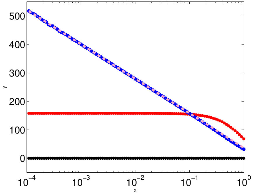
After some algebra, Eq. (13) reduces to
| (15) |
where the dimensionless functions still involve four angular integrals and are given in the Appendix. The integrals are performed numerically using Monte-Carlo sampling. The function diverges logarithmically with vanishing , as shown in Fig. 2, It is well fitted by , while the other two integrals take on a constant value, therefore the limit can safely be taken. Upon using scaling with the number of Monte-Carlo steps, and is found, as also visualized in Fig. 2. By -power counting, the term contains the lowest power, thus is the most dominant at low temperatures, where only the low energy dynamics around the Weyl point matters.
Keeping only the dominant term and performing the remaining integrals, we eventually obtain
These are valid at low temperatures and small chemical potential (i.e. smaller than the bandwidth).
V The hyperfine coupling and Overhauser field
Since our electronic system consist of non-interacting fermions, the conventional Korringa relation [24] between the relaxation rate and the density of states (DOS) is expected to be recovered, namely . The DOS for Weyl semimetals is with is the volume of the unit cell. By introducing an effective, energy dependent hyperfine coupling as
| (18) |
the above relation is satisfied. This identification of the hyperfine coupling is further justified by comparing to Eq. (11), with which it agrees apart from the numerical prefactor. This means that the hyperfine coupling in Weyl semimetals is tunable by doping or gate voltage. For large velocity and gyromagnetic ratio (17 MHz/T for 31P) and small unit cell and doping or temperature, it can be of the order of 100 eV. Close to the Weyl point, the hyperfine coupling is sizeable but the DOS is vanishingly small, while away from the Weyl point, the DOS is enhanced significantly at the expense of reducing the hyperfine coupling. This suggests that the nuclear spins are not relaxed through Weyl fermions but by some other, non-intrinsic mechanism. Weyl semimetals often contain NMR active nuclei (e.g. P, Nb, Ta) with very high natural abundance, and at low energies, The coupling in Eq. (18) predicts a strongly enhanced Overhauser field between the nuclear and electron spins, which is tunable by gate voltages. Such tunability can be useful in controlling coherence in quantum dot devices containing Weyl fermions for quantum information or spintronical devices. In particular, the lifting of the spin blockade in a double quantum dot device by Overhauser fields[25] can be manipulated by the gate tunability of the hyperfine fields of Weyl systems.
Besides the logarithmic term, Eq. (IV) resembles closely to the nuclear spin relaxation time in graphene[22, 23], where the same and powers arise from the linearly vanishing DOS in 2D. As opposed to that, the DOS in Weyl semimetals varies with the square of the energy and its interplay with the diverging hyperfine interaction produces a graphene like spin relaxation time with additional log-corrections. A similar logarithmic Larmor frequency dependence arises in the Hebel-Slichter NMR peak in s-wave superconductors[26] or in density waves[27] due to the divergence of the density of states at the gap edge. A constant hyperfine coupling, coming from the spin-dipole term (the function in Eq. (15)), produces indeed a subleading scaling.
Finally we comment on the Knight shift, i.e. the shift of the position of the magnetic resonance signal. Neglecting the orbital effect of the magnetic field on Weyl fermions, as we have done throughout this paper, a Zeeman term, should be added to Eq. (1). The effect of on within first order perturbation theory determines the Knight shift. However, the magnetic field shifts the Weyl node in the momentum-space by an amount , so that the spin density remains unchanged. This is analogous to the vanishing spin susceptibility of Weyl fermions[28] within the realm of the low energy theory, Eq. (1).
Let us note that the NMR response of a nuclear spin usually resembles closely to the behaviour of a magnetic impurity in a metallic host at high temperatures, well above the Kondo temperature. This originates from the fact that in both cases, the hyperfine interaction and the Heisenberg exchange term are represented by a constant coupling. In the present case, however, this mapping ceases to be exact due to the peculiar divergence of the orbital part of the hyperfine interaction.
VI Conclusions
We have focused on the hyperfine interaction in Weyl fermions, and the ensuing NMR dynamics. While the spin-dipole part of the coupling behaves conventionally as in other metals, the orbital contribution is found to be tunable by gating or doping the system and diverges anomalously at the vicinity of the Weyl point with the inverse energy. This promises to be relevant for controlling the lifting of the spin blockade in double quantum dot devices[25]. The spin lattice relaxation time behaves as with the nuclear Larmor frequency and . This a) differs from naive expectation by an factor due to the anomalous orbital hyperfine coupling in Weyl systems, and b) is logarithmically enhanced by the Larmor frequency. This resembles to the scaling of the Hebel-Slichter peak in s-wave superconductors.
Acknowledgements.
BD is supported by the Hungarian Scientific Research Fund Nos. K101244, K105149, K108676.Appendix A The Fourier transform of the hyperfine coupling
We Fourier transform Eq. (9) term by term. The first term, originating from the interaction between the nuclear spin and the orbital motion of the electron, involves , where denotes the Fourier transform as
| (19) |
This is calculated after realizing that the integrand, is the negative gradient of , i.e. the Coulomb potential. After partial integration, we are left with
| (20) |
where . Analogously to the Fourier transform of the Coulomb interaction in 3D from the Yukawa potential, this integral is evaluated as limit of
| (21) |
which yields
| (22) |
Similarly to how the Fourier transform of the Coulomb interaction behaves in various dimensions[29], the graphene case[23] in 2D contains only a single term in the denominator of Eq. (22).
The Fourier transform of the Zeeman term proceeds along similar steps. The spin dipole term can be rewritten in terms of directional derivatives as [30]
| (23) |
where is the directional derivative. The Fourier transform of the last term containing the Dirac-delta function gives trivially one.
Appendix B The matrix element of nuclear spin flip
The matrix element, appearing in Eq. (13) is obtained by selecting only those terms from Eq. (11), which contain the and components of the nuclear spin, giving and . These define , which eventually yields
| (24) |
where in spherical coordinates, we have
| (25) | |||
| (26) | |||
| (27) |
and similarly for with the restriction due to the Dirac delta in Eq. (13), and . Additionally,
| (28) | |||
| (29) |
We have also defined
| (30) |
, and similarly for . In particular,
| (31) | |||
| (32) | |||
| (33) |
Appendix C The , and functions
First, we define the auxiliary functions
| (35) | |||
| (36) | |||
| (37) |
with from Eq. (14). By multiplying them with , stemming from the Jacobian, and integrating them with respect to the four angular variables , from 0 to and , from 0 to , we get the desired , and functions. The resulting dimensionless functions depend only on the ratio , which is denoted by , and not separately on and .
References
- [1] B. A. Bernevig, T. L. Hughes, and S.-C. Zhang, Quantum spin hall effect and topological phase transition in hgte quantum wells, Science 314, 1757 (2006).
- [2] M. König, S. Wiedmann, C. Brune, A. Roth, H. Buhmann, L. W. Molenkamp, X.-L. Qi, and S.-C. Zhang, Quantum spin hall insulator state in hgte quantum wells, Science 318, 766 (2007).
- [3] M. Z. Hasan and C. L. Kane, Colloquium : Topological insulators, Rev. Mod. Phys. 82, 3045 (2010).
- [4] X.-L. Qi and S.-C. Zhang, Topological insulators and superconductors, Rev. Mod. Phys. 83, 1057 (2011).
- [5] C. Herring, Accidental degeneracy in the energy bands of crystals, Phys. Rev. 52, 365 (1937).
- [6] X. Wan, A. M. Turner, A. Vishwanath, and S. Y. Savrasov, Topological semimetal and fermi-arc surface states in the electronic structure of pyrochlore iridates, Phys. Rev. B 83, 205101 (2011).
- [7] S. Murakami, Phase transition between the quantum spin hall and insulator phases in 3d: emergence of a topological gapless phase, New Journal of Physics 9(9), 356 (2007).
- [8] A. A. Burkov and L. Balents, Weyl semimetal in a topological insulator multilayer, Phys. Rev. Lett. 107, 127205 (2011).
- [9] A. H. Castro Neto, F. Guinea, N. M. R. Peres, K. S. Novoselov, and A. K. Geim, The electronic properties of graphene, Rev. Mod. Phys. 81, 109 (2009).
- [10] C.-L. Zhang, S.-Y. Xu, I. Belopolski, Z. Yuan, Z. Lin, B. Tong, G. Bian, N. Alidoust, C.-C. Lee, S.-M. Huang, T.-R. Chang, G. Chang, et al., Signatures of the adler-bell-jackiw chiral anomaly in a weyl fermion semimetal, Nat. Commun. 7, 10735 (2016).
- [11] X. Huang, L. Zhao, Y. Long, P. Wang, D. Chen, Z. Yang, H. Liang, M. Xue, H. Weng, Z. Fang, X. Dai, and G. Chen, Observation of the chiral-anomaly-induced negative magnetoresistance in 3d weyl semimetal taas, Phys. Rev. X 5, 031023 (2015).
- [12] S.-Y. Xu, I. Belopolski, N. Alidoust, M. Neupane, G. Bian, C. Zhang, R. Sankar, G. Chang, Z. Yuan, C.-C. Lee, S.-M. Huang, H. Zheng, et al., Discovery of a weyl fermion semimetal and topological fermi arcs, Science (2015).
- [13] S.-M. Huang, S.-Y. Xu, I. Belopolski, C.-C. Lee, G. Chang, B. Wang, N. Alidoust, G. Bian, M. Neupane, C. Zhang, S. Jia, A. Bansil, et al., A weyl fermion semimetal with surface fermi arcs in the transition metal monopnictide taas class, Nat. Commun. 6, 7373 (2015).
- [14] L. Lu, Z. Wang, D. Ye, L. Ran, L. Fu, J. D. Joannopoulos, and M. Soljačić, Experimental observation of weyl points, Science (2015).
- [15] J. Winter, Magnetic Resonance in Metals (Clarendon Press, Oxford, 1971).
- [16] A. Abragam, Principles of Nuclear Magnetism (Clarendon Press, Oxford, 1961).
- [17] C. P. Slichter, Principles of Magnetic Resonance (Spinger-Verlag, New York, 1989), 3rd ed.
- [18] L. C. Hebel and C. P. Slichter, Nuclear Spin Relaxation in Normal and Superconducting Aluminum, Phys. Rev. 113, 1504 (1959).
- [19] Y. Maeno, T. M. Rice, and M. Sigrist, The intriguing superconductivity of strontium ruthenate, Phys. Today 54, 42 (2001).
- [20] I. Žutić, J. Fabian, and S. D. Sarma, Spintronics: Fundamentals and applications, Rev. Mod. Phys. 76, 323 (2004).
- [21] M. Neupane, S. Xu, R. Sankar, N. Alidoust, G. Bian, C. Liu, I. Belopolski, T.-R. Chang, H.-T. Jeng, H. Lin, A. Bansil, F. Chou, et al., Observation of a three-dimensional topological dirac semimetal phase in high-mobility cd3as2, Nat. Commun 5, 3786 (2014).
- [22] B. Dóra and F. Simon, Unusual hyperfine interaction of dirac electrons and nmr spectroscopy in graphene, Phys. Rev. Lett. 102, 197602 (2009).
- [23] B. Dóra and F. Simon, Hyperfine interaction in graphene: The relevance for spintronics, physica status solidi (b) 247, 2935 (2010).
- [24] H. Alloul, Nmr studies of electronic properties of solids, Scholarpedia 9, 32069 (2014).
- [25] O. N. Jouravlev and Y. V. Nazarov, Electron transport in a double quantum dot governed by a nuclear magnetic field, Phys. Rev. Lett. 96, 176804 (2006).
- [26] M. Tinkham, Introduction to Superconductivity (MacGraw-Hill, New York, 1996).
- [27] T. Maniv, Effect of a spin density wave instability on the nuclear spin-lattice relaxation in quasi 1-d conductors, Solid State Commun. 43, 47 (1982).
- [28] M. Koshino and I. F. Hizbullah, Magnetic susceptibility in three-dimensional nodal semimetals, Phys. Rev. B 93, 045201 (2016).
- [29] T. Giamarchi, Quantum Physics in One Dimension (Oxford University Press, Oxford, 2004).
- [30] S. Jiang, L. Greengard, and W. Bao, Fast and accurate evaluation of nonlocal coulomb and dipole-dipole interactions via the nonuniform fft, SIAM J. Sci. Comput 36, B777 (2014).