Periodically-driven Kondo impurity in nonequilibrium steady states

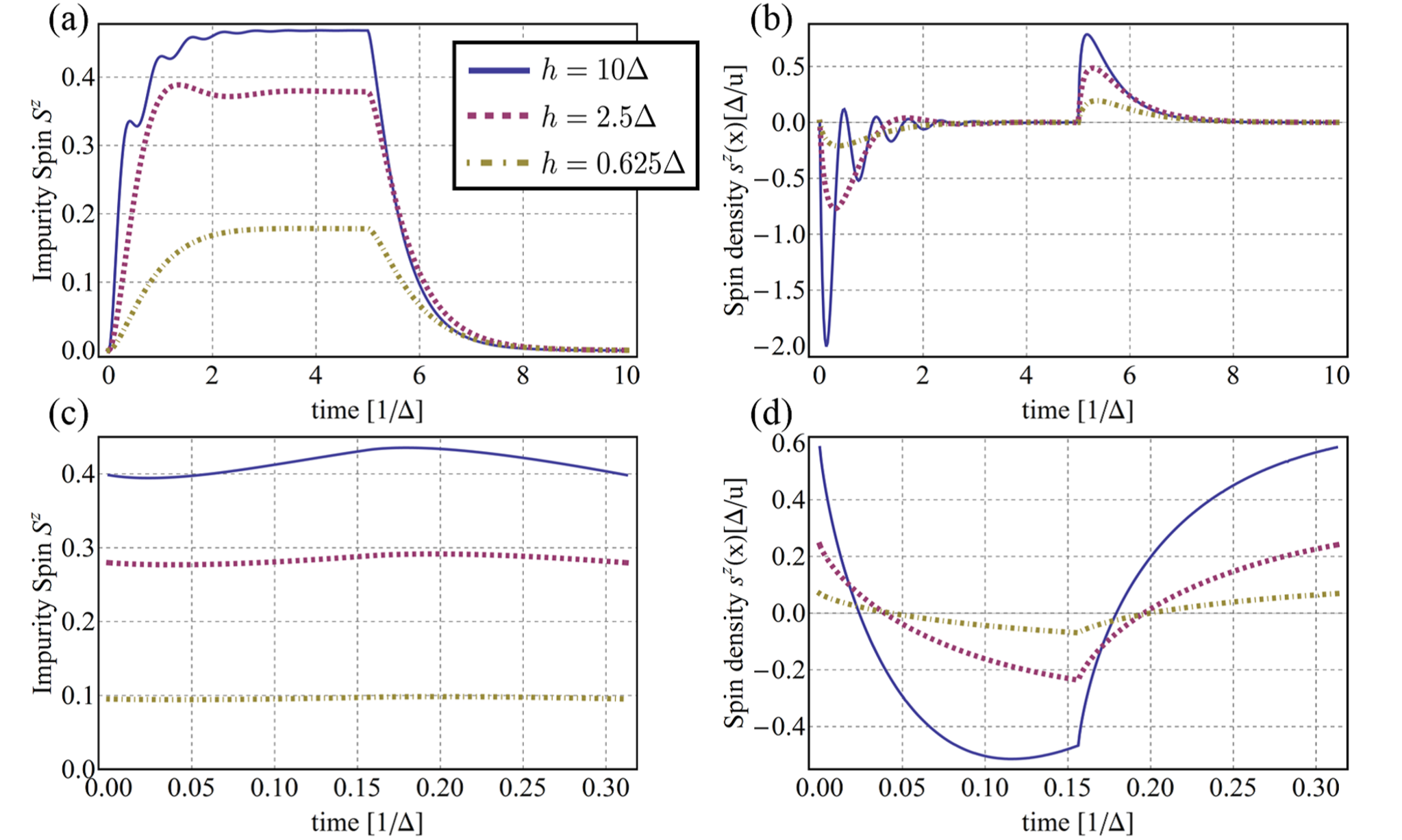
Here, we discuss a specific case: the local magnetic field is periodically switched on and off. Note that the following analysis and discussion can be straightforwardly applied to more generic periodically driven systems. The time dependence of $h(t)$ we consider is

Decompose time into periodic intervals: $t=N\tau+s,\ N\in\mathbb{N},\ 0<s<\tau$. Then, the time evolution of the impurity spin polarization in the steady state in the long-time limit is

The prefactors $A_{i}^{(\prime)}(s)$ can be obtained by the momentum integral in the fermionic-bath sector. The second term is the relaxation term due to the switching of the field intensity. The third term in $0<s<\tau/2$ represents the oscillation caused by the local magnetic field, which comes from the interference between the impurity spin and the spins in the fermionic bath. Recall that the spin density of the fermionic bath is represented by the time derivative of the impurity spin polarization (see Eq. (8)).

The time evolution of the impurity spin polarization $\braket{S^{z}(t)}$ and the spin density of the fermionic bath $\braket{s^{z}(x,t)}$ in a period are shown in Fig. 1. Because the impurity spin polarization $\braket{S^{z}(t)}$ is time periodic in the steady state, the spin density of fermionic bath $\braket{s^{z}(x,t)}$ is spatially periodic as well as time periodic, as seen from Eq. (8). We thus show only the data at the point $x=Mu\tau\ (M\in\mathbb{N})$. In the first half of the period the local magnetic field is switched on (i.e. $h(t)=h$), while in the second half it is off (i.e. $h(t)=0$). In the long driving period (see the figures of $\tau=10/\Delta$), the impurity spin polarization oscillates with a frequency proportional to the field intensity $h$, and eventually relaxes to its equilibrium value in the time scale proportional to $1/T_{K}$. Wave packets whose width is of the order of the inverse of the Kondo temperature are observed in the spin density of the fermionic bath since the spin density of the fermionic bath is given by the time derivative of the impurity spin polarization. These wave packets propagate with the Fermi velocity $u$ without decaying due to the linear dispersion. In the short driving period (see the figures of $\tau=0.3125/\Delta$), the system cannot keep up with the temporal change of the local magnetic field and thus approaches constant values. Note that a large cusp is observed at a half of the period in the spin density of the fermionic bath, because it is given by the time derivative of the impurity spin polarization and thus amplified by the factor $\Omega=2\pi/\tau$.

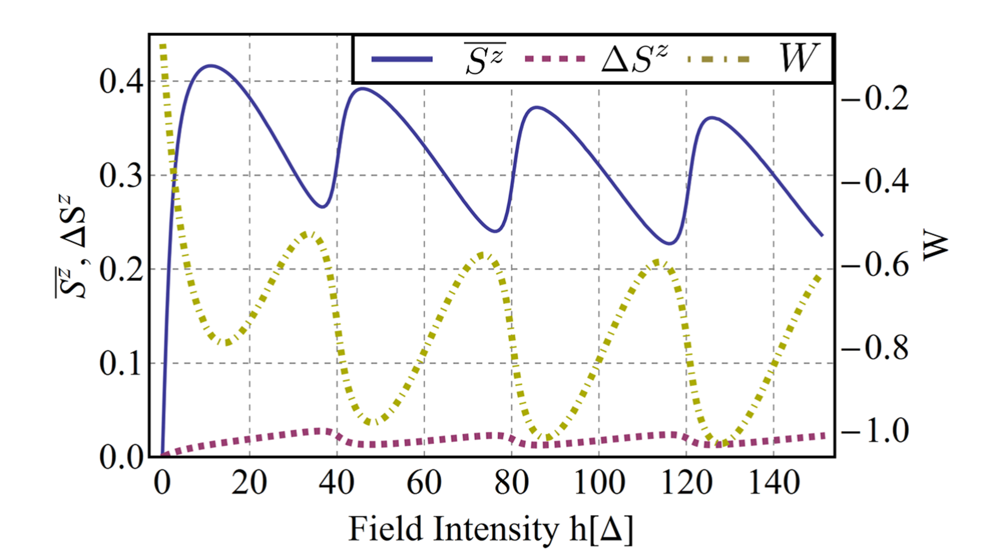
In the limit of fast driving, the impurity spin polarization $\braket{S^{z}(t)}$ approaches a temporally constant value (see Fig. 1). Under this condition, we investigate how the time average of the impurity spin polarization, $\overline{S^{z}}$, depends on the local magnetic field intensity $h$, and elucidate their intriguing resonance phenomenon. Here we define the time average $\overline{S^{z}}$ and its variance $\Delta S^{z}$:

where $\lim_{N\rightarrow\infty}$ is taken to extract the steady state.

The obtained results are shown in Fig. 2 as a function of the field intensity $h$ for a choice of the driving period, $\tau=0.3125\Delta$. Naively, we expect that $\overline{S^{z}}$ increases monotonically and saturates to $1/2$ with increasing $h$. Interestingly, however, an emergent oscillation is observed as a function of $h$ and its period is determined by the driving period of the local magnetic field. When $h\gg T_{K}$, the time average of the impurity spin polarization $\overline{S^{z}}(h)$ becomes periodic as a function of $h$

where $\tau$ is the driving period of the local magnetic field.

To see the essence of this behavior, let us define the “power” $P$ and the “work done in a period” $W$ for this system, based on an analogy to the power in classical mechanics,

It is expected that $dS^{z}/dt$ corresponds to the velocity of a particle $v=dx(t)/dt$, and $dh(t)/dt$ corresponds to the force $F$ in classical mechanics, that is, the following correspondence to classical mechanics is expected:

The quantity $W$ is shown as a function of $h$ in Fig. 2. The emergent oscillation in the time average of the impurity spin polarization as a function of $h$ can be attributed to a resonance phenomenon between the oscillation of the impurity spin polarization (see Fig. 1) and switching of the local magnetic field. The impurity spin polarization oscillates with the period of $2\pi/h$ in the first half of the period, and the local magnetic field is switched off just at the half of the period. Analogy to an oscillator in classical mechanics would suggest that if the time derivative of the impurity spin polarization is negative at the half of the period where the local magnetic field is switched off, the amplitude toward the negative direction would become larger, and therefore the time average would be smaller. Note that the “work done in a period” $W$ oscillates with the same period but an opposite phase, whereas the variance of the impurity spin polarization $\overline{S^{z}}$ is small but oscillates with the same phase as the “work”. These behaviors are indeed consistent with our interpretation. The resonance condition deduced by the analogy mentioned above is

which reproduces the period observed in Fig. 2.

Here, we consider a specific case where the time dependence of the local magnetic field $h(t)$ and the in-plane interaction parameter $J_{\perp}(t)$ is given by

Note that the time dependence of the local magnetic field $h(t)$ equals that of the square of the in-plane interaction parameter $J_{\perp}^{2}(t)$, which has the essence of dynamics when both the local magnetic field and the in-plane interaction parameter are time dependent. The dynamics of the impurity spin polarization in the steady state is

where $J_{n}(z)$ is the integer Bessel function. Because $A(t+\tau/2)=A(t)$, the impurity spin polarization is time periodic whose period is half of the driving period $\tau$: $\braket{S^{z}(t+\tau/2)}=\braket{S^{z}(t)}$. This is because the in-plane interaction parameter acts as an effective hopping parameter, and thereby the square of the in-plane interaction parameter appears in the observables.

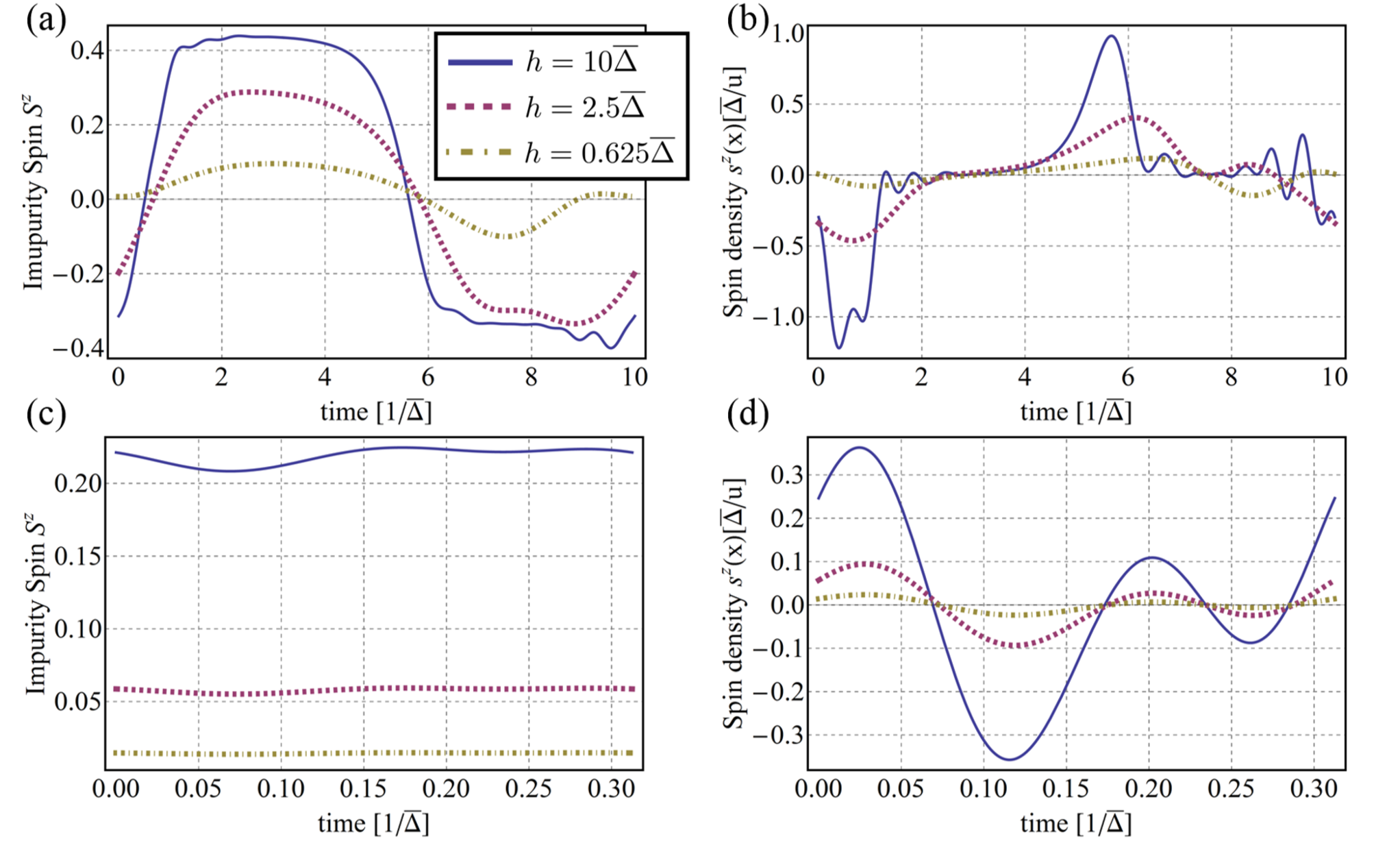
In Fig. 3, we show the time evolution of the impurity spin polarization $\braket{S^{z}(t)}$ and the spin density of a fermionic bath $\braket{s^{z}(x,t)}\ (x=Mu\tau,\ M\in\mathbb{N})$ in a half of the driving period. Let us define the effective Kondo temperature by $T_{K}^{\text{eff}}=\pi w\overline{\Delta}$ (see Appendix B for the meaning of this definition). When the driving period is much longer than the time scale of the inverse of the effective Kondo temperature (see the figures of $\tau=20/\overline{\Delta}$), the system follows a temporal change in the external driving in the time scale of $1/T_{K}^{\text{eff}}$. Therefore, the behavior of time evolution is similar to the case without in-plane interaction driving (see Sec. III). When the driving period is much smaller than the inverse of the effective Kondo temperature (see the figures of $\tau=0.625/\overline{\Delta}$), these values also approach temporally constant values as we have seen for the case without in-plane interaction driving.

It should be noted, however, that the time average of the impurity spin polarization does not vanish even though the local magnetic field does not have the static component (i.e. zeroth mode of Fourier coefficients). This is because the square of the in-plane interaction parameter becomes small while the local magnetic field is negative. Namely, the impurity spin is effectively decoupled from the fermionic bath when the local magnetic field is negative. In the high frequency limit $(\overline{\Delta}/\Omega\rightarrow 0)$, the time average of impurity spin polarization is $\overline{S^{z}}=\sum_{n\in\mathbb{N}}J_{n}(h/2\Omega)J_{n+1}(h/2\Omega)$. This behavior is consistent with the results by Heyl and Kehrein [33] in the linear response regime when the coupling term is periodically switched on and off.

We now demonstrate that intriguing steady states appear in the high frequency limit. The following analysis is valid for any type of time dependence of $h(t)$ and $J_{\perp}(t)$. Note that the time evolution of the system is determined solely by the function $T_{dk}(t)$ in the steady state (see Eq. (30)), so it is sufficient to study the properties of $T_{dk}(t)$. In the language of the resonant level model, $T_{dk}(t)$ denotes a transition matrix from a state with wave-number $k$ in the fermionic bath to the resonant level. For arbitrary $h(t)$ and $J_{\perp}(t)$, each element of the transition matrix $T_{dk}(t)$ is represented as,

where $\overline{f}=\int_{0}^{\tau}f(t)dt/\tau$ is a time average in a period and the coefficients $\tilde{J}^{(n)}$ and $F(t)$ are determined from the Fourier coefficients of the external driving $h(t)$ and $J_{\perp}(t)$. The transition matrix without driving $T_{dk}^{\text{bare}}(t)$ in the long time limit is

Thus, $T_{dk}^{(n)}(t)$ can be interpreted as a ”$n$th photon assisted transition matrix”.

By taking the high frequency limit $(\overline{\Delta}/\Omega,\ \overline{h}/\Omega\rightarrow 0)$, the impurity-spin polarization $\braket{S^{z}(t)}$ and the impurity-spin time correlation function, $\braket{S^{z}(t)S^{z}(t^{\prime})}$, recover time translational invariance. We thus end up with the analysic formuae in this limit,

where $\Delta^{(n)}=|\tilde{J}^{(n)}|^{2}/4\pi\alpha u$. In the equilibrium Kondo model with a local magnetic field $h$ at Toulouse limit and temperature $T$, the impurity-spin polarization $\braket{S^{z}}_{eq}$ and the impurity-spin time correlation function [67, 68] $\braket{S^{z}(t)S^{z}}_{eq}$ are expressed as follows:

where $f(\epsilon)=1/(e^{\epsilon}+1)$ is the Fermi distribution function.

Comparison between Eq. (20) and Eq. (21) gives instructive implications for the asymptotic states. Because $f(\omega\Delta/T)\xrightarrow{T\rightarrow 0}\theta(-\omega)$ and $f(\omega\Delta/T)\xrightarrow{T\rightarrow\infty}\frac{1}{2}$, the integrals from $-\infty$ to $0$ in Eq. (20) have the properties of the zero temperature state (the time correlation function shows a power law decay $\braket{S^{z}(t)S^{z}(t^{\prime})}\propto(t-t^{\prime})^{-2}\ (t\gg t^{\prime})$), while the integrals from $-\infty$ to $\infty$ in Eq. (20) have the properties of the infinite temperature state (the time correlation function shows an exponential decay $\braket{S^{z}(t)S^{z}(t^{\prime})}\propto e^{-2\overline{\Delta}|t-t^{\prime}|}$). Thus, the properties of the system are described by a mixture of the zero-temperature state and those of the infinite-temperature state in general. This means that the reservoir we consider here cannot prevent the localized spin from heating up completely. The properties of the zero temperature state come from the bare transitions (i.e. transition processes without photons) while the properties of the infinite temperature come from the photon-assisted transition processes. If $\Delta^{(0)}=0$ and $\Delta^{(n)}=\Delta^{(-n)}$ $(\Delta^{(n\neq 0)}=0)$ the properties of the system are described by those at zero (infinite) temperature, respectively. In these special cases, the asymptotic state can be described by the equilibrium state.

Two concrete examples exhibiting either zero- or infinite-temperature properties for asymptotic states are in order here. First, consider the case where the local magnetic field is sinusoidal $h(t)=h\sin(\Omega t)$ and the in-plane interaction is time independent, $\tilde{J}^{(n)}=J_{n}(h/\Omega)$. Then, the impurity-spin polarization and the impurity-spin time correlation function are exactly reduced to those of the infinite temperature state for the intensities $h$ which satisfy the zeros of the zeroth Bessel function. This is easily confirmed from Eq. (20), where we can put $\Delta^{(0)}=0$. The second example is the $h(t)/\Omega\rightarrow 0$ case: if we take the limit of $h(t)/\Omega\rightarrow 0$, then $\tilde{J}^{(n)}=J_{\perp}^{(n)}$, where $J_{\perp}^{(n)}$ is the $n$th Fourier coefficient of $J_{\perp}(t)$. In this case, the steady state cannot be described by the time averaged Hamiltonian even though the frequency of the external driving is set to infinity. While the impurity-spin polarization and the impurity-spin time correlation function are exactly equivalent to those of the infinite-temperature state when $J_{\perp}^{(0)}=0\ (\Leftrightarrow\overline{J_{\perp}}=0)$, they are exactly equivalent to those of the zero-temperature state when $J_{\perp}^{(n)}=0\ (\forall n\neq 0)\ (\Leftrightarrow J_{\perp}\text{ is time independent})$. The other cases cannot be described effectively by any equilibrium systems due to the fluctuation dissipation theorem [33].

To close this section, we make a brief comment on the nonequilibrium Fermi distribution function. Note that the above asymptotic behaviors originate from the duplication of the Fermi edge (or equivalently duplication of the impurity level) [69, 70]. In calculating observables, we evaluate $\braket{\tilde{c}^{\dagger}_{d}(t)\tilde{c}_{d}(t^{\prime})}$, which can be written down explicitly as,

The above observation enables us to define the nonequilibrium distribution function $f_{\text{noneq}}(\beta\epsilon)\propto\sum_{n}|\tilde{J}^{(n)}|^{2}f(\beta(\epsilon+n\Omega))$. The nonequilibrium distribution function has Fermi edges at $\epsilon=n\Omega\ (n\in\mathbb{N})$ and the weight of each edge is $|\tilde{J}^{(n)}|^{2}$. Because the Fermi edge at $\epsilon=0$ can pick up the contribution of the density of states of the resonant level and the others cannot, a transition without photons results in the zero-temperature behavior while the others result in the infinite temperature behavior.

References

- [1] D. Goldhaber-Gordon, H. Shtrikman, D. Mahalu, D. Abusch-Magder, U. Meirav, and M. A. Kastner, Nature 391, 156 (1998a).
- [2] D. Goldhaber-Gordon, J. Göres, M. A. Kastner, H. Shtrikman, D. Mahalu, and U. Meirav, Phys. Rev. Lett. 81, 5225 (1998b).
- [3] Cronenwett, Sara M. and Oosterkamp, Tjerk H. and Kouwenhoven, Leo P., Science 281, 540 (1998).
- [4] J. Schmid, J. Weis, K. Eberl, and K. v. Klitzing, Physica B 256–258, 182 (1998).
- [5] A. Schirotzek, C.-H. Wu, A. Sommer, and M. W. Zwierlein, Phys. Rev. Lett. 102, 230402 (2009).
- [6] S. Nascimbène, N. Navon, K. J. Jiang, L. Tarruell, M. Teichmann, J. McKeever, F. Chevy, and C. Salomon, Phys. Rev. Lett. 103, 170402 (2009).
- [7] S. Will, T. Best, S. Braun, U. Schneider, and I. Bloch, Phys. Rev. Lett. 106, 115305 (2011).
- [8] M. Koschorreck, D. Pertot, E. Vogt, B. Frohlich, M. Feld, and M. Kohl, Nature 485, 619 (2012).
- [9] C. Kohstall, M. Zaccanti, M. Jag, A. Trenkwalder, P. Massignan, G. M. Bruun, F. Schreck, and R. Grimm, Nature 485, 615 (2012), 1112.0020 .
- [10] J. Bauer, C. Salomon, and E. Demler, Phys. Rev. Lett. 111, 215304 (2013).
- [11] Y. Nishida, Phys. Rev. Lett. 111, 135301 (2013).
- [12] M. Nakagawa and N. Kawakami, Phys. Rev. Lett. 115, 165303 (2015).
- [13] J. Catani, G. Lamporesi, D. Naik, M. Gring, M. Inguscio, F. Minardi, A. Kantian, and T. Giamarchi, Phys. Rev. A 85, 023623 (2012).
- [14] T. Fukuhara, A. Kantian, M. Endres, M. Cheneau, P. Schauß, S. Hild, D. Bellem, U. Schollwöck, T. Giamarchi, C. Gross, I. Bloch, and S. Kuhr, Nat. Phys. 9, 235 (2013a), 1209.6468 .
- [15] T. Fukuhara, P. Schauß, M. Endres, S. Hild, M. Cheneau, I. Bloch, and C. Gross, Nature 502, 76 (2013b), 1305.6598 .
- [16] S. Hild, T. Fukuhara, P. Schauß, J. Zeiher, M. Knap, E. Demler, I. Bloch, and C. Gross, Phys. Rev. Lett. 113, 147205 (2014).
- [17] A. Kogan, S. Amasha, and M. A. Kastner, Science 304, 1293 (2004).
- [18] C. Latta, F. Haupt, M. Hanl, A. Weichselbaum, M. Claassen, W. Wuester, P. Fallahi, S. Faelt, L. Glazman, J. von Delft, H. E. Tureci, and A. Imamoglu, Nature 474, 627 (2011).
- [19] P. Nordlander, M. Pustilnik, Y. Meir, N. S. Wingreen, and D. C. Langreth, Phys. Rev. Lett. 83, 808 (1999).
- [20] D. Lobaskin and S. Kehrein, Phys. Rev. B 71, 193303 (2005).
- [21] F. B. Anders and A. Schiller, Phys. Rev. Lett. 95, 196801 (2005).
- [22] F. B. Anders and A. Schiller, Phys. Rev. B 74, 245113 (2006).
- [23] M. H. Hettler and H. Schoeller, Phys. Rev. Lett. 74, 4907 (1995).
- [24] T.-K. Ng, Phys. Rev. Lett. 76, 487 (1996).
- [25] A. Schiller and S. Hershfield, Phys. Rev. Lett. 77, 1821 (1996).
- [26] Y. Goldin and Y. Avishai, Phys. Rev. Lett. 81, 5394 (1998).
- [27] P. Nordlander, N. S. Wingreen, Y. Meir, and D. C. Langreth, Phys. Rev. B 61, 2146 (2000).
- [28] R. López, R. Aguado, G. Platero, and C. Tejedor, Phys. Rev. Lett. 81, 4688 (1998).
- [29] Y. Goldin and Y. Avishai, Phys. Rev. B 61, 16750 (2000).
- [30] A. Kaminski, Y. V. Nazarov, and L. I. Glazman, Phys. Rev. Lett. 83, 384 (1999).
- [31] A. Kaminski, Y. V. Nazarov, and L. I. Glazman, Phys. Rev. B 62, 8154 (2000).
- [32] R. López, R. Aguado, G. Platero, and C. Tejedor, Phys. Rev. B 64, 075319 (2001).
- [33] M. Heyl and S. Kehrein, Phys. Rev. B 81, 144301 (2010).
- [34] M. Knap, A. Shashi, Y. Nishida, A. Imambekov, D. A. Abanin, and E. Demler, Phys. Rev. X 2, 041020 (2012).
- [35] M. Knap, D. A. Abanin, and E. Demler, Phys. Rev. Lett. 111, 265302 (2013).
- [36] T. Oka and H. Aoki, Phys. Rev. B 79, 081406 (2009).
- [37] Lindner, Netanel H. and Refael, Gil and Galitski, Victor, Nat Phys 7, 490 (2011).
- [38] T. Kitagawa, T. Oka, A. Brataas, L. Fu, and E. Demler, Phys. Rev. B 84, 235108 (2011).
- [39] M. Aidelsburger, M. Atala, M. Lohse, J. T. Barreiro, B. Paredes, and I. Bloch, Phys. Rev. Lett. 111, 185301 (2013).
- [40] H. Miyake, G. A. Siviloglou, C. J. Kennedy, W. C. Burton, and W. Ketterle, Phys. Rev. Lett. 111, 185302 (2013).
- [41] W. Magnus, Comm. Pure Appl. Math. 7, 649 (1954).
- [42] S. Blanes, F. Casas, J. Oteo, and J. Ros, Physics Reports 470, 151 (2009).
- [43] L. D’Alessio and M. Rigol, Phys. Rev. X 4, 041048 (2014).
- [44] A. Lazarides, A. Das, and R. Moessner, Phys. Rev. E 90, 012110 (2014).
- [45] P. Ponte, A. Chandran, Z. Papić, and D. A. Abanin, Ann. Phys. (N. Y.) 353, 196 (2015).
- [46] T. Mori, Phys. Rev. A 91, 020101 (2015).
- [47] D. A. Abanin, W. De Roeck, and F. Huveneers, Phys. Rev. Lett. 115, 256803 (2015).
- [48] T. Kuwahara, T. Mori, and K. Saito, Annals of Physics 367, 96 (2016).
- [49] T. Mori, T. Kuwahara, and K. Saito, Phys. Rev. Lett. 116, 120401 (2016).
- [50] S. Kohler, T. Dittrich, and P. Hänggi, Phys. Rev. E 55, 300 (1997).
- [51] H.-P. Breuer, W. Huber, and F. Petruccione, Phys. Rev. E 61, 4883 (2000).
- [52] W. Kohn, J. Stat. Phys. 103, 417 (2001).
- [53] D. W. Hone, R. Ketzmerick, and W. Kohn, Phys. Rev. E 79, 051129 (2009).
- [54] R. Ketzmerick and W. Wustmann, Phys. Rev. E 82, 021114 (2010).
- [55] T. Iadecola, C. Chamon, R. Jackiw, and S.-Y. Pi, Phys. Rev. B 88, 104302 (2013).
- [56] M. Langemeyer and M. Holthaus, Phys. Rev. E 89, 012101 (2014).
- [57] T. Iadecola, T. Neupert, and C. Chamon, Phys. Rev. B 91, 235133 (2015).
- [58] T. Shirai, T. Mori, and S. Miyashita, Phys. Rev. E 91, 030101 (2015).
- [59] D. E. Liu, Phys. Rev. B 91, 144301 (2015).
- [60] T. Iadecola and C. Chamon, Phys. Rev. B 91, 184301 (2015).
- [61] T. Shirai, J. Thingna, T. Mori, S. Denisov, P. Hänggi, and S. Miyashita, New Journal of Physics 18, 053008 (2016).
- [62] G. Toulouse, C. R. Acad. Sci. B 268, 1200 (1969).
- [63] I. Affleck and A. W. Ludwig, Nucl. Phys. B 360, 641 (1991).
- [64] G. Zaránd and J. von Delft, Phys. Rev. B 61, 6918 (2000).
- [65] T. Giamarchi, Quantum Physics in One Dimension, International Series of Monographs on Physics (Clarendon Press, 2003).
- [66] N. S. Wingreen, A.-P. Jauho, and Y. Meir, Phys. Rev. B 48, 8487 (1993).
- [67] F. Guinea, Phys. Rev. B 32, 4486 (1985).
- [68] A. J. Leggett, S. Chakravarty, A. T. Dorsey, M. P. A. Fisher, A. Garg, and W. Zwerger, Rev. Mod. Phys. 59, 1 (1987).
- [69] P. K. Tien and J. P. Gordon, Phys. Rev. 129, 647 (1963).
- [70] S. Kohler, J. Lehmann, and P. Hänggi, Physics Reports 406, 379 (2005).