Stationary state of a zero-range process corresponding to multifractal one-particle distribution
Abstract
We investigate a zero-range process where the underlying one-particle stationary distribution has multifractality. The multiparticle stationary probability measure can be written in a factorized form. If the number of the particles is sufficiently large, a great part of the particles condense at the site with the highest measure of the one-particle problem. The number of the particles out of the condensate scales algebraically with the system size and the exponent depends on the strength of the disorder. These results can be well reproduced by a branching process, with similar multifractal property.
pacs
05.40.-a, 05.60.CdI Introduction
It has been well known that disorder may change the behavior of the system, not only quantitatively but also qualitatively, in stochastic systems, as well as in classical or quantum spin systems and the quantum localization problem[1, 2]. The effect of disorder is more remarkable when the spatial dimension of the system is lower. For example, at one-particle level, a localization where a particle stays at a certain specific site with much higher probability than at the other sites[3], and a phase separation, where the regions with high particle density and low particle density are separated spontaneously[4], are well known phenomena.
In many cases, the disorder which is considered is a random disorder: A disorder is represented as identically and independently distributed (i.i.d.) stochastic variables and thus, by definition, these variables are not spatially correlated each other. In a real situation, however, disorder may be spatially correlated and it is valuable to consider a model with spatially correlated disorder.
Aperiodic disorder is a class of disorder with spatial correlation. An aperiodic disorder is generated deterministically from a set of specific rules. That is the point which distinguishes an aperiodic disorder from random disorder and which enables us to study systems with aperiodic disorder systematically. Therefore study of systems with aperiodic disorder is a good first step toward understanding of more general system with spatially correlated disorder. Although some investigations have been carried out about the effect of aperiodic disorder in classical and quantum spin chains[5, 6, 7, 8] so far, to our knowledge, just a few in stochastic systems. It has been known that even at one-particle level, an interesting behavior can be observed: An anomalous diffusion where the variance grows less slowly than linear growth in time [9] and correspondingly the stationary probability distribution with multifractality[10]. Note that systems with aperiodic disorder are not only of theoretical and mathematical interest, but also they have been artificially fabricated and investigated experimentally[11].
One of the next interesting problems is to make clear an interplay between quenched disorder with spatial correlation and interaction between particles. For this purpose we study a simple multiparticle stochastic process, called the zero-range process (ZRP)[12] with aperiodic disorder. In ZRP, it is remarkable that the exact stationary measure can be written in a factorized form, which is derived from the one-particle stationary probability distribution. Moreover, under a certain condition, condensation can be observed, where a great part of the particles condense at one specific site. The effect of random quenched disorder in ZRP has already been investigated[13, 14]. In this paper, specifically, we consider ZRP with disorder constructed from an aperiodic sequence, called the paperfolding (PF) sequence[15]. This is one of the models where a multifractal stationary probability distribution can be observed.
II A zero-range process with aperiodic disorder
Let us consider a one-dimensional lattice with periodic boundary condition. Each site can accommodate any number of particles. A particle hops from site to site with designated hop rates and only hopping to one of the nearest neighboring sites is allowed. The hop rates are quenched variables, where we denote the forward rate from site to by and the backward rate from to by (see Fig.1).

Here we assume that the hop rates do not depend on the number of particles at the departure site (sometimes called the ”pure chipping process”[16]), although generally the hop rates in ZRP are given by a function of the number of particles at the departure site. For example, in a noninteracting particle system the hop rates are directly proportional to the number of particles at the departure site.
Let us construct the aperiodic disorder according to the PF sequence. The PF sequence is generated systematically by the initial sequence and the substitution rules, , , , and . The length of the sequence of the -th generation, , is and in the limit the ratio of the number of A’s, , to that of B’s, , converges to unity. Then the hop rates are assigned as
| (1) |
and
| (2) |
At one-particle level, the drift velocity is proportional to the difference between unity and the product of [17]
| (3) |
The state of the multiparticle system is specified by the particle configuration , where denotes the number of particles at site . The total number of particles, is conserved, since the periodic boundary condition is imposed.
Let denote the probability that the configuration is observed at time . The master equation is given as
| (4) | |||||
One of the remarkable features of ZRP is that the exact multiparticle stationary measure can be obtained, from the one-particle distribution (the stationary probability that the particle exist at the -th site), in a factorized form:
| (5) |
where denotes the partition function
| (6) |
The symbol indicates that the total number of particles is fixed at .
The one-particle distribution is given by the stationary solution of the master equation describing the random walk on the lattice:
| (7) |
It is known that the stationary solution can be obtained analytically[17]:
| (8) |
where
| (9) |
III Condensation and scaling of the number of particles out of condensate
Figure 2 shows the density profile obtained from Monte Carlo simulations.


When the average density is low, the interaction between particles is ineffective and the profile shows a hierarchical structure, as observed for the one-particle distribution (see Fig.2(a)). On the other hand, when the average density increases, many particles condense at the site which gives the maximum of the one-particle distribution (see Fig.2(b)). This condensation is already known to occur for randomly disordered case. An analogy to the Bose-Einstein condensation is pointed out[12].
In order to study the condensation in more detail, we introduce the grand-canonical(GC) formulation. In the GC formulation, the grand partition function is given in a factorized form:
| (11) | |||||
where denotes the fugacity. Then the local density at site is obtained as
| (12) |
The average density is given as
| (13) |
From these expressions, it is immediately understood that the density of the site, at which the maximum of the one-particle distribution is given, rapidly increases, since at the site, as increases, the numerator of Eq.(12) increases most rapidly and the denominator decreases most rapidly. However, for a finite system, Eqs.(12) and (13) can take any finite value for . Therefore, the GC formulation cannot be broken as long as we consider a finite system. As is well known, condensation is characterized by the breaking of the GC formulation. Then it is necessary to consider the thermodynamic limit where with fixed to be finite.
In the thermodynamic limit, the expression of the total density Eq.(13) is rewritten as
| (14) | |||||
where the summation in the r.h.s. of Eq.(13) is replaced with the integral, and denotes the distribution function of . A condensation can occur if the integral converges in the limit . For the integral to converge, the distribution function must be an increasing function of in the neighborhood of . In the case where the one-particle distribution has multifractality, this condition is considered to be satisfied. However, it is still quite difficult to calculate the integral and evaluate the critical density at which the condensation occurs. This consideration is similar to that for the density of states near the lowest energy level in Bose-Einstein condensation. Hereafter, we consider the case where the total density is large enough for the condensation to occur in the thermodynamic limit.
The total number of particles out of the condensate, , is evaluated as
| (15) | |||||
where is the condensation site and in the last line the fugacity is replaced with .
Figure 3 shows the dependence of on the system size for , , and . It is found that increases algebraically with respect to :
| (16) |
where the power-law exponent depends on . This result is qualitatively different from that in the case with random disorder, where is kept , independent of the system size[13]. This can be considered as one of the characteristic results generated by the spatially correlated aperiodic disorder and interaction between particles.
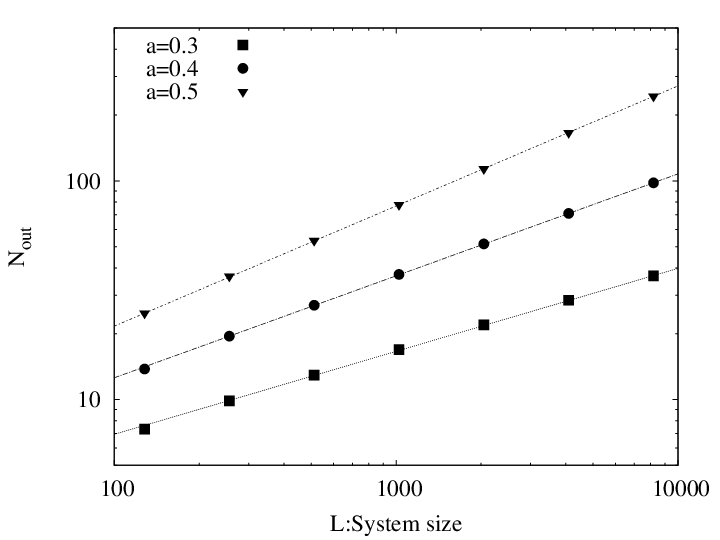
Figure 4 shows the dependence of the exponent on . It is a monotonically increasing function: The stronger the disorder, the smaller the exponent. However, we are not sure about the values to which the exponent converges in the (extremely strong disorder) and (extremely weak disorder) limits. It is quite difficult to obtain them numerically, since for some measures are quite small, and for the difference of the measures is quite small.

In our previous study, we found that the multifractal structure of the one-particle distribution can be well reproduced by the binomial branching process (BBP)[10]. This process is constructed by the iteration of dividing the segments into two halves and uneven partitioning of the measure by assiging one segment to and the other to [18], where , assumed to be , is the only free parameter of the process. The disorder strength of the PF model, , and the parameter can be related through the multifractal singular exponent:
| (17) |
For the distribution generated by the BBP with , which corresponds to the given disorder strength , we evaluate through Eq.(15). The evaluated also shows a power-law dependence on the system size , similar to that for the PF model. Moreover, the exponent agrees very well, as shown in Fig.4. The one-particle distributions themselves for these two processes are not so similar each other, although their multifractal structures are similar. This suggests that the multifractal structure of the one-particle distributionis essential. It should be noted that for the PF model the structure is resulted from the aperiodic disorder.
IV Summary
We investigated a phenomena emerged by both an aperiodic disorder and interaction between particles using the ZRP with disorder according to the PF sequence, for which the underlying one-particle stationary distribution is multifractal. In the stationary state, when the density is sufficiently high, a condensation occurs, where most particle condense at one specific site. For a finite size system, the number of particles out of the condensate increases with the system size algebraically, contrary to the randomly disordered case where it is suppressed to . The distribution generated by the BBP has a similar multifractality and can reproduce the exponent well. This is a characteristic result by an interplay between the effects of spatially correlated disorder and that of the interaction between particles.
Acknowledgements.
This research was supported by the initiative-based project E-05 ”Creation and Sustainable Governance of New Commons through Foundation of Integrated Local Environmental Knowledge (ILEK)”, Research Institute for Humanity and Nature (RIHN).References
- [1] R.B.Stinchcombe, Adv.Phys. 50, 431(2001).
- [2] F.Iglói and C.Monthus, Physics Reports 412, 277(2005).
- [3] J.-P.Bouchard and A.Georges, Physics Reports 195, 127(1990).
- [4] J.Krug, Braz.J.Phys. 30, 97(1997).
- [5] J.M.Luck, J.Stat.Phys. 72, 417(1993).
- [6] J.Hermisson, J.Phys.A 33, 57(2000).
- [7] A.P.Vieira, Phys.Rev.Lett. 94, 077201(2005).
- [8] K.Hida, Phys.Rev.Lett. 93, 037205(2004).
- [9] F.Iglói, L.Turban and H.Rieger, Phys.Rev.E 59, 1465(1999).
- [10] H.Miki, Phys.Rev.E 89, 062105(2014).
- [11] L.Dal Negro, J.H.Yi.V.Nguyen, Y.Yi.J.Michel and L.C.Kimerling, Appl.Phys.Lett. 86, 261905(2005); V.Passias, N.V.Valappil, Z.Shi, L.Deych, A.A.Lisyansky and V.M.Menon, Opt.Exp. 17, 6636(2009).
- [12] M.R.Evans and T.Hanney, J.Phys.A 38, R195(2005).
- [13] R.Juhasz, L.Santen, and F.Iglói, Phys.Rev.E 72, 046129(2005).
- [14] C.Godreche and J.M.Luck, J.Stat.Mech. P12013(2012).
- [15] M.Dekking, Theor.Comput.Sci. 414, 20(2012).
- [16] E.Levine, D.Mukamel, and G.M.Schütz, J.Stat.Phys. 120, 759(2005).
- [17] B.Derrida, J.Stat.Phys. 31, 433(1983).
- [18] C.Meneveau and K.R.S.Sreenivasan, Phys.Rev.Lett. 59, 1424(1987).