The Radial Velocity Experiment (RAVE): Fifth Data ReleaseNote: accepted by AJ, 15 Nov 2016
Abstract
Data Release 5 (DR5) of the Radial Velocity Experiment (RAVE) is the fifth data release from a magnitude-limited () survey of stars randomly selected in the southern hemisphere. The RAVE medium-resolution spectra () covering the Ca-triplet region (8410-8795 Å) span the complete time frame from the start of RAVE observations in 2003 to their completion in 2013. Radial velocities from 520 781 spectra of 457 588 unique stars are presented, of which 255 922 stellar observations have parallaxes and proper motions from the Tycho-Gaia astrometric solution (TGAS) in Gaia DR1. For our main DR5 catalog, stellar parameters (effective temperature, surface gravity, and overall metallicity) are computed using the RAVE DR4 stellar pipeline, but calibrated using recent K2 Campaign 1 seismic gravities and Gaia benchmark stars, as well as results obtained from high-resolution studies. Also included are temperatures from the Infrared Flux Method, and we provide a catalogue of red giant stars in the dereddened color interval (0.50,0.85) for which the gravities were calibrated based only on seismology. Further data products for sub-samples of the RAVE stars include individual abundances for Mg, Al, Si, Ca, Ti, Fe, and Ni, and distances found using isochrones. Each RAVE spectrum is complemented by an error spectrum, which has been used to determine uncertainties on the parameters. The data can be accessed via the RAVE Web site or the Vizier database.
Subject headings
surveys — stars: abundances, distancesI. Introduction
The kinematics and spatial distributions of Milky Way stars help define the Galaxy we live in, and allow us to trace parts of the formation of the Milky Way. In this regard, large spectroscopic surveys that provide measurements of fundamental structural and dynamical parameters for a statistical sample of Galactic stars, have been extremely successful in advancing the understanding of our Galaxy. Recent and ongoing spectroscopic surveys of the Milky Way include the RAdial Velocity Experiment [101, RAVE,], the Sloan Extension for Galactic Understanding and Exploration [115, SEGUE,], the APO Galactic Evolution Experiment [42, APOGEE,], the LAMOST Experiment for Galactic Understanding and Exploration [116, LAMOST,], the Gaia–ESO Survey [48, GES,] and the GALactic Archaeology with HERMES [41, GALAH,]. These surveys were made possible by the emergence of wide field multi-object spectroscopy (MOS) fibre systems, technology that especially took off in the 1990s. Each survey has its own unique aspect, and together form complementary samples in terms of capabilities and sky coverage.
Of the above mentioned surveys, RAVE was the first, designed to provide stellar parameters to complement missions that focus on astrometric information. The four previous data releases, DR1 [101], DR2 [117], DR3 [98] and DR4 [68] have been the foundation for a number of studies which have advanced our understanding of especially the disk of the Milky Way [70, see review by]. For example, in recent years a wave-like pattern in the stellar velocity distribution was uncovered [109] and the total mass of the Milky Way was measured using the RAVE extreme-velocity stars [86], as was the local dark matter density [14, 87]. Moreover, chemo-kinematic signatures of the dynamical effect of mergers on the Galactic disk [77], and signatures of radial migration were detected [69, 110]. Stars tidally stripped from globular clusters were also identified [66, 4, 5]. RAVE further allowed for the creation of pseudo-3D maps of the diffuse interstellar band at 8620 Å [67] and high-velocity stars to be studied [54].
RAVE DR5 includes not only the final RAVE observations taken in 2013, but also earlier discarded observations recovered from previous years, resulting in an additional RAVE spectra. This is the first RAVE data release in which error spectrum was generated for each RAVE observation, so we can provide realistic uncertainties and probability distribution functions for the derived radial velocities and stellar parameters. We have performed a recalibration of stellar metallicities, especially improving stars of super-solar metallicity. Using the Gaia benchmark stars [61, 55] as well as 72 RAVE stars with Kepler-2 asteroseismic parameters (Valentini et al. submitted, hereafter V16), the RAVE values have been recalibrated, resulting in more accurate gravities especially for the giant stars in RAVE. The distance pipeline [15] has been improved and extended to process more accurately stars with low metallicities (). Finally, by combining optical photometry from APASS [80] with 2MASS [102] we have derived temperatures from the Infrared Flux Method [33].
Possibly the most unique aspect of DR5 is the extent to which it complements the first significant data release from Gaia. The successful completion of the Hipparcos Mission and publication of the catalogue [43] demonstrated that space astrometry is a powerful technique to measure accurate distances to astronomical objects. Already in RAVE-DR1[101], we looked forward to the results from the ESA cornerstone mission Gaia, as this space-based mission’s astrometry of Milky Way stars will have 100 times better astrometric accuracies than its predecessor, Hipparcos. Although Gaia has been launched and data collection is ongoing, a long enough time baseline has to have elapsed for sufficient accuracy of a global reduction of observations [75, e.g., five years for Gaia to yield positions, parallaxes and annual proper motions at an accuracy level of 5 – 25 as,]. To expedite the use of the first Gaia astrometry results, the approximate positions at the earlier epoch (around 1991) provided by the Tycho-2 Calalogue [56] can be used to disentangle the ambiguity between parallax and proper motion in a shorter stretch of Gaia observations. These TGAS stars therefore contain positions, parallaxes, and proper motions earlier than the global astrometry from Gaia can be released. There are unique RAVE stars in TGAS, so for these stars we now have space-based parallaxes and proper motions from Gaia DR1 in addition to stellar parameters, radial velocities, and in many cases chemical abundances. The Tycho-2 stars observed by RAVE in a homogeneous and well-defined manner can be combined with the released TGAS stars to exploit the larger volume of stars for which milliarcsecond accuracy astrometry exists, for an extraordinary return in scientific results. We note that in a companion paper, a data-driven re-analysis of the RAVE spectra using The Cannon model has been carried out (Casey et al. 2016, in prep, hereafter C16), which presents the derivation of , surface gravity and , as well as chemical abundances of giants of up to seven elements (O, Mg, Al, Si, Ca, Fe, Ni).
In §II, the selection function of the RAVE DR5 stars is presented – further details can be found in Wojno et al. submitted, hereafter W16. The RAVE observations and reductions are summarised in §III. An explanation of how the error spectra were obtained is found in §IV, and §V summarises the derivation of radial velocities from the spectra. In §VI, the procedure used to extract atmospheric parameters from the spectrum is described and the external verification of the DR5 , and [M/H] values is discussed in §VII. The dedicated pipelines to extract elemental abundances, and distances are described in §§VIII and IX, respectively – DR5 gives radial velocities for all RAVE stars but elemental abundances and distances are given for sub-samples of RAVE stars that have SNR 20 and the most well-defined stellar parameters. Temperatures from the Infrared Flux Method are presented in §X. In §XI we present for the red giants gravities based on asteroseismology by the method of V16. A comparison of the stellar parameters in the RAVE DR5 main catalog to other stellar parameters for RAVE stars (e.g., those from C16) is provided in §XII. The final sections, §XIII and §XIV provide a summary of the difference between DR4 and DR5, and an overview of DR5, respectively.
II. Survey Selection Function
Rigorous exploitation of DR5 requires knowledge of RAVE’s selection function, which was recently described by W16. Here we provide only a summary.
The stars for the RAVE input catalogue were selected from their -band magnitudes, focusing on bright stars () in the southern hemisphere, but the catalogue does contain some stars that are either brighter or fainter, in part because stars were selected by extrapolating data from other sources, such as Tycho-2 and SuperCOSMOS before DENIS was available in 2006 [see DR4 paper, 68, §2 for details]. As the survey progressed, the targets in the input catalog were grouped into four -band magnitude bins: 9.0 – 10.0, 10.0 – 10.75, 10.75 – 11.5, and 11.5 – 12.0, which helped mitigate fibre cross-talk problems. This led to a segmented distribution of RAVE stars in -band magnitudes, but the distributions in other passbands are closely matched by Gaussians [80, see e.g., Fig. 11 in]. For example, in the -band, the stars observed by RAVE have a nicely Gaussian distribution, peaking at with .
The initial target selection was based only on the apparent -band magnitude, but a colour criterion () was later imposed in regions close to the Galactic plane (Galactic latitude ) to bias the survey towards giants. Therefore, the probability, , of a star being observed by the RAVE survey is
| (1) |
where is Galactic longitude. W16 determine the function both on a field-by-field basis, so time-dependent effects can be captured, and with Hierarchical Equal-Area iso-Latitude Pixelisation (HEALPix) [51, e.g.,], which divides the sky into equal-area pixels, as regularly distributed as possible. The sky is divided into 12 288 pixels () which results in a pixel area of , and we only consider the selection function evaluated with HEALPix, because RAVE fields overlap on the sky for quality control and variability tests.
The parent RAVE sample is constructed by first discarding all repeat observations, keeping only the observation with the highest SNR. Then observations which were not conducted as part of the typical observing strategy (e.g., calibration fields) were removed. Finally, all stars with that were observed despite violating the colour criterion were dismissed. After applying these cuts, we are left with 448 948 stars, or 98% of all stars targeted by RAVE. These define the RAVE DR5 core sample (survey footprint). The core sample is complemented by targeted observations (e.g., open clusters), mainly for calibration and testing.
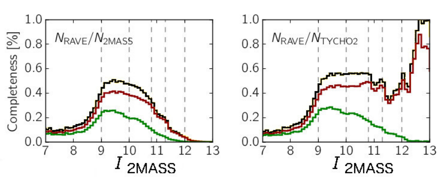
The number of RAVE stars () in each HEALPix pixel is then counted as a function of . We apply the same criteria to two photometric all-sky surveys, 2MASS and Tycho-2 to discover how many stars could, in principle, have been observed. After these catalogues were purged of spurious measurements, we obtain and and can compute the completeness of RAVE as a function of magnitude for both 2MASS and TYCHO2 as and .
Figure 1 shows the DR5 completeness with respect to Tycho-2 as a function of magnitude. It is evident that RAVE avoids the Galactic plane, and we find that the coverage on the sky is highly anisotropic, with a significant drop-off in completeness at the fainter magnitudes. A similar result is seen for (W16). However, in , there is a significantly higher completeness at low Galactic latitudes () for the fainter magnitude bins.
Because stars that passed the photometric cuts were randomly selected for observation, RAVE DR5 is free of kinematic bias. Hence, the contents of DR5 are representative of the Milky Way for the specific magnitude interval. A number of peculiar and rare objects are included. The morphological flags of Matijevič et al. [74] allow one to identify the normal single stars (90 - 95%), and those that are unusual – the peculiar stars include various types of spectroscopic binary and chromospherically active stars. The stars falling within the RAVE selection function footprint described in W16 are provided in 10.17876/rave/dr.5/005.

III. Spectra and their Reduction
The RAVE spectra were taken using the multi-object spectrograph 6dF (6 degree field) on the m UK Schmidt Telescope of the Australian Astronomical Observatory (AAO). A total of 150 fibres could be allocated in one pointing, and the covered spectral region (8410–8795 Å) at an effective resolution of was chosen as analogous to the wavelength range of Gaia’s Radial Velocity Spectrometer [see DR1 paper, 101, §2 and §3 for details].
The RAVE reductions are described in detail in DR1 §4 and upgrades to the process are outlined in DR3 §2. In DR5 further improvements have been made to the Spectral Parameters And Radial Velocity (SPARV) pipeline, the DR3 pipeline that carries out the continuum normalisation, masks bad pixels, and provides RAVE radial velocities. The most significant is that instead of the reductions being carried out on a field-by-field basis, single fibre processing was implemented. Therefore, if there were spectra within a RAVE field which simply could not be processed, instead of the whole field failing and being omitted in the final RAVE catalogue, only the problematic spectra are removed. This is one reason DR5 has more stars than the previous RAVE data releases.
The DR5 reduction pipeline is able to processes the problematic DR1 spectra, and it produces error spectra. An overhaul of bookkeeping and process control lead to identification of multiple copies of the same observation and of spectra with corrupted FITS headers. Some RAVE IDs have changed from DR4, and some stars released in DR4 could not be processed by the DR5 pipeline. The vast majority of these stars have low signal-to-noise ratios (). Details are provided in Appendix A; less than 0.1% of RAVE spectra were affected by bookkeeping inconsistencies.
| in DR5 | |
|---|---|
| RAVE stellar spectra | 520,781 |
| Unique stars observed | 457,588 |
| Stars with visits | 8000 |
| Spectra / unique stars with | 478,161 / 423,283 |
| Spectra / unique stars with | 66,888 / 60,880 |
| Stars with a | 428,952 |
| Stars with elemental abundances | 339,750 |
| Stars with morphological flags n,d,g,h,o | 394,612 |
| Tycho2 + RAVE stellar spectra/unique stars | 309,596 / 264,276 |
| TGAS + RAVE stellar spectra/unique stars | 255 922 / 215,590 |
| aFor a discussion of AlgoConv see §VI.1 |
IV. Error Spectra
The wavelength range of the RAVE spectra is dominated by strong spectral lines: for a majority of stars, the dominant absorption features are due to the infra-red calcium triplet (CaT), which in hot stars gives way to Paschen series of hydrogen. Also present are weaker metallic lines for the Solar type stars and molecular bands for the coolest stars. Within an absorption trough the flux is small, so shot noise is more significant in the middle of a line than in the adjacent continuum. Error levels increase also at wavelengths of airglow sky emission lines, which have to be subtracted during reductions. As a consequence, a single number, usually reported as a SNR ratio, is not an adequate quantification of the observational errors associated with a given spectrum.
For this reason, DR5 provides error spectra which comprise uncertainties (“errors”) for each pixel of the spectrum. RAVE spectra generally have a high SNR in the continuum (its median value is SNR ), and there shot noise dominates the errors. Denoting number of counts accumulated in the spectrum before sky subtraction by , the corresponding number after sky subtraction by , and the effective gain by , the shot noise is and the signal is . The appearance of rather than in the relation for reflects the fact that noise is enhanced near night-sky emission lines. As a consequence the SNR ratio is decreased both within profiles of strong stellar absorption lines (where is small) and near sky emission lines. The gain is determined using the count vs. magnitude relation [117, see eq. 1 from ]. Its value () reflects systematic effects on a pixel-to-pixel scale that lower the effective gain to this level.
Telluric absorptions are negligible in the RAVE wavelength range [79]. RAVE observations from Siding Spring generally show a sky signal with a low continuum level, even when observed close to the Moon. The main contributors to the sky spectrum are therefore airglow emission lines, which belong to three series: OH transitions 6-2 at Å, OH transitions 7-3 at Å, and O2 bands at Å. Wavelengths of OH lines are listed in the file linelists$skylines.dat which is part of the IRAF11 1 IRAF is distributed by the National Optical Astronomy Observatory, which is operated by the Association of Universities for Research in Astronomy (AURA) under a cooperative agreement with the National Science Foundation. reduction package, while the physics of their origin is nicely summarised at http://www.iafe.uba.ar/aeronomia/airglow.html. One needs to be careful when analysing stellar lines with superimposed airglow lines. Apart from increasing the noise levels, these lines may not be perfectly subtracted, as they can be variable on angular scales of degrees and on timescales of minutes, whereas the telescope’s field of view is and the exposure time was typically 50 minutes.
Evaluation of individual reduction steps [117, see] shows that fibre cross-talk and scattered light have only a small influence on error levels. In particular, a typical level of fibre-cross talk residuals is , where is the ratio between flux of an object in an adjacent fibre and flux of the object in question. Fibre cross-talk suffers from moderate systematic effects (variable point spread function profiles across the wavelength range), but even at the edges of the spectral range these effects do not exceed a 1% level. Scattered light typically contributes % of the flux level of the spectral tracing. So its effect on noise estimation is not important, and we were not able to identify any systematics. Finally, RAVE observes in the near IR and uses a thinned CCD chip, so an accurate subtraction of interference fringes is needed. Tests show that fringe patterns for the same night and for the same focal plate typically stay constant to within 1% of the flat-field flux level. As a result scattered light and fringing only moderately increase the final noise levels. Together, scattered light and fringing are estimated to contribute a relative error of %, which is added in quadrature to the prevailing contribution of shot noise discussed above.
Finally we note that fluxes and therefore noise levels for individual pixels of a given spectrum are not independent of each other, but are correlated because of a limited resolving power of RAVE spectra. So the final noise spectrum was smoothed with a window with a width of 3 pixels in the wavelength direction, which corresponds to the FWHM for a resolving power of RAVE spectra.
For each pixel in a RAVE spectrum, we invoke a Gaussian with a mean and standard deviation as measured from the same pixel of the corresponding error spectra. A new spectrum is therefore generated which can be roughly interpreted as an alternative measurement of the star (although note the error spectrum does not take every possible measurement uncertainty into account as discussed above). We then can redetermine our radial velocity for these resampled data which will differ slightly from that obtained from the actual observed spectrum. Repeating this resampling process and monitoring the resulting radial velocity estimates, we get a distribution of the radial velocity from which we can then infer an uncertainty.
The raw errors as derived in the error spectra are propagated both into the radial velocities and stellar parameters presented here. This process allows a better assessment of the uncertainties, especially of stars with low SNR or hot stars, where the CaT is not as prominent. Figure 2 shows the mean radial velocity from the resulting radial velocity estimates of 100 resampled spectra for low SNR stars. For most RAVE stars, the radial velocity errors are consistent with a Gaussian (see middle panel), but for the more problematic hot stars, or those with low SNR, this is clearly not the case.
Each RAVE spectrum was resampled from its error spectrum ten times. Whereas our tests indicate that a larger number of resamplings () would be ideal for the more problematic spectra, ten resamplings were chosen as a compromise between computing time and the relatively small number of RAVE spectra with low SNR and hot stars that would benefit from additional resamplings. For % of the RAVE sample, there is one-sigma or less difference in the radial velocity and radial velocity dispersions when resampling the spectrum 10 or 100 times. In DR5, we provide both the formal error in radial velocity, which is a measure of how well the cross-correlation of the RAVE spectrum against a template spectrum was matched, and the standard deviation and the median absolute deviation (MAD) in heliocentric radial velocity from a spectrum resampled ten times.
Each RAVE spectrum was resampled from its error spectrum ten times. Whereas our tests indicate that a larger number of resamplings () would be ideal for the more problematic spectra, ten resamplings were chosen as a compromise between computing time and the relatively small number of RAVE spectra with low SNR and hot stars that would benefit from additional resamplings. For % of the RAVE sample, there is one-sigma or less difference in the radial velocity and radial velocity dispersions when resampling the spectrum 10 or 100 times.
V. Radial Velocities
The DR5 radial velocities are derived in an identical manner to in those in DR4. The process of velocity determination is explained by Siebert et al. [98]. Templates are used to measure the radial velocities in a two-step process. First, using a subset of 10 template spectra, a preliminary estimate of the RV is obtained, which has a typical accuracy better than 5 km s-1. A new template is then constructed using the full template database described in Zwitter et al. [117], from which the final, more precise RV is obtained. This has a typical accuracy better than 2 km s-1.
The internal error in RV, , comes from the xcsao task within IRAF, and therefore describes the error on the determination of the maximum of the correlation function. It was noticed that for some stars, particularly those with , was underestimated. The inclusion of error spectra in DR5 largely remedies this problem, and the standard deviation and MAD provide independent measures of the RV uncertainties (see Fig. 2). Uncertainties derived from the error spectra are especially useful for stars that have low SNR or high temperatures. Figure 3 shows the errors from the resampled spectra compared to the internal errors. For the majority of RAVE stars, the uncertainty in RV is dominated by the cross-correlation between the RAVE spectrum and the RV template, and not by the array of uncertainties (“errors”) for each pixel of the RAVE spectrum.
Repeated RV measurements have been used to characterise the uncertainty in the RVs. There are 43 918 stars that have been observed more than once; the majority (82%) of these stars have two measurements, and six RAVE stars were observed 13 times. The histogram of the RV scatter between the repeat measurements peaks at 0.5 km s-1, and has a long tail at larger scatter. This extended scatter is due both to variability from stellar binaries and problematic measurements. If stars are selected that have radial velocities derived with high confidence, e.g., stars with , , and [68, see], the scatter of the repeat measurements peaks at and the tail is reduced by 90%.
The zero-point in RV has already been evaluated in the previous data releases. The exercise is repeated here, with the inclusion of a comparison to APOGEE and Gaia-ESO, and the summary of the comparisons to different samples is given in Table 2. Our comparison sample comprises of the GCS [82] data as well as high-resolution echelle follow-up observations of RAVE targets at the ANU 2.3 m telescope, the Asiago Observatory, the Apache Point Observatory [93], and Observatoire de Haute Provence using the Elodie and Sophie instruments. Sigma-clipping is used to remove contamination by spectroscopic binaries or problematic measurements, and the mean given is . As seen previously, the agreement in zero-point between RAVE and the external sources is better than 1 km s-1.
| Sample | (, | ||
|---|---|---|---|
| GCS | 1020 | 0.31 | 1.76 (3,113) |
| Chubak | 97 | 0.07 | 1.28 (3,2) |
| Ruchti | 443 | 0.79 | 1.79 (3,34) |
| Asiago | 47 | 0.22 | 2.98 (3,0) |
| ANU 2.3m | 197 | 0.58 | 3.13 (3,16) |
| OHP Elodie | 13 | 0.49 | 2.45 (3,2) |
| OHP Sophie | 43 | 0.83 | 1.58 (3,4) |
| APOGEE | 1121 | 0.11 | 1.87 (3,144) |
| Gaia-Eso | 106 | 0.14 | 1.68 (3,15) |
VI. Stellar Parameters and Abundances
VI.1. Atmospheric parameter determinations
RAVE DR5 stellar atmospheric parameters, , and have been determined using the same stellar parameter pipeline as in DR4. The details can be found in Kordopatis et al. [65] and the DR4 paper [68], but a summary is provided here.
The pipeline is based on the combination of a decision tree, DEGAS [13], to renormalise iteratively the spectra and obtain stellar parameter estimations for the low SNR spectra, and a projection algorithm MATISSE [91] to derive the parameters for stars having high SNR. The threshold above which MATISSE is preferred to DEGAS is based on tests performed with synthetic spectra [65, see] and has been set to SNR=30 pixel-1.
The learning phase of the pipeline is carried out using synthetic spectra computed with the Turbospectrum code [3] combined with MARCS model atmospheres [52] assuming local thermodynamic equilibrium (LTE) and hydrostatic equilibrium. The cores of the CaT lines are masked in order to avoid issues such as non-LTE effects in the observed spectra, which could affect our parameter determination.
The stellar parameters covered by the grid are between 3000 K and 8000 K for , 0 and 5.5 for and 5 to +1 dex in metallicity. Varying -abundances () as a function of metallicity are also included in the learning grid, but are not a free parameter. The line-list was calibrated on the Sun and Arcturus [65].
The pipeline is run on the continuum normalised, radially-velocity corrected RAVE spectra using a soft conditional constraint based on the 2MASS colours of each star. This restricted the solution space and minimised the spectral degeneracies that exist in the wavelength range of the CaT [65]. Once a first set of parameters is obtained for a given observation, we select pseudo-contrinuum windows to re-normalize the input spectrum based on the pseudo-continuum shape of the synthetic spectrum having the parameters determined by the code, and the pipeline is run again on the modified input. This step is repeated ten times, which is usually enough for convergence of the continuum shape to be reached and hence to obtain a final set of parameters (see, however, next paragraph).
Once the spectra have been parameterised, the pipeline provides one of the four quality flags for each spectrum22 2 The flags are unchanged as compared to DR4.:
- •
‘0’: The analysis was carried out as desired. The re-normalisation process converged, as did MATISSE (for high SNR spectra) or DEGAS (for low SNR spectra).
- •
‘1’: Although the spectrum has a sufficiently high SNR to use the projection algorithm, the MATISSE algorithm did not converge. Stellar parameters for stars with this flag are not reliable. Approximately 6% of stars are affected by this.
- •
‘2’: The spectrum has a sufficiently high SNR to use the projection algorithm, but MATISSE oscillates between two solutions. The reported parameters are the mean of these two solutions. In general the oscillation happens for a set of parameters that are nearby in parameter space and computing the mean is a sensible thing to do. However, this is not always the case, for example, if the spectrum contains artefacts. Then the mean may not provide accurate stellar parameters. Spectra with a flag of ‘2’ could be used for analyses, but with caution.
- •
‘3’: MATISSE gives a solution that is extrapolated from the parameter range of the learning grid, and the solution is forced to be the one from DEGAS. For spectra having artefacts but high-SNR overall, this is a sensible thing to do, as DEGAS is less sensitive to such discrepancies. However, for the few hot stars that have been observed by RAVE, adopting this approach is not correct. A flag of ‘3’ and a 7750 K is very likely to indicate that this is a hot star with 8000 K and hence that the parameters associated with that spectrum are not reliable.
- •
‘4’: This flag will only appear for low SNR stars. For metal-poor giants, the spectral lines available are neither strong enough nor numerous enough to have DEGAS successfully parametrise the star. Tests on synthetic spectra have shown that to derive reliable parameters the settings used to explore the branches of the decision tree need to be changed compared to the parameters adopted for the rest of the parameter space. A flag ‘4’ therefore marks this change in the setting for book-keeping purposes, and the spectra associated with this flag should be safe for any analysis.
The several tests performed for DR4 as well as the sub-sequent science papers, have indicated that the stellar parameter pipeline is globally robust and reliable. However, being based on synthetic spectra that may not match the real stellar spectra over the entire parameter range, the direct outputs of the pipeline need to be calibrated on reference stars in order to minimise possible offsets.
VI.2. Metallicity calibrations
In DR4, metallicity calibration proved to be the most critical and important one. Using a set of reference stars for which metallicity determinations were available in the literature (usually derived from high-resolution spectra), a second order polynomial correction, based on surface gravity and raw metallicity, was applied in DR4. This corrected the metallicity offsets with the external datasets of Pasquini et al. [85], Pancino et al. [84], Cayrel et al. [38], Ruchti et al. [93] and the PASTEL database [99]. For DR5, we relied on the same approach. However, we added reference stars to the set used in DR4, with the focus on expanding our calibrating sample towards the high metallicity end to better calibrate the tails of the distribution function. This calibration is based on the crossmatch of RAVE targets with the Worley et al. [112] and Adibekyan et al. [1] catalogues, as well as the Gaia benchmark stellar spectra. The metallicity of the Gaia benchmark stars is taken from Jofré et al. [61], where a library of Gaia benchmark stellar spectra was specially prepared to match RAVE data in terms of wavelength coverage, resolution and spectral spacing. This was done following the procedure described in Blanco-Cuaresma et al. [18]. Our calibration has already been successfully used in Kordopatis et al. [71], Wojno et al. [110] and Antoja et al. (submitted). The calibration relation for DR5 is:
| (2) |
where is the calibrated metallicity, and are, respectively, the uncalibrated (raw output from the pipeline) metallicity and surface gravity. The effect of the calibration on the raw output can be seen in the top panel of Fig. 4. The bottom panel shows that in the range the DR5 and DR4 values are very similar. Above 0, the DR5 metallicities are higher than the DR4 ones and are in better agreement with the chemical abundance pipeline presented below (§VIII). We note that after metallicity calibration we do not re-run the pipeline to see if other stellar parameters change with this new metallicity.


VI.3. Surface gravity calibrations
Measuring the surface gravity spectroscopically, and in particular from medium resolution spectra around the IR calcium triplet, is challenging. Nevertheless, the DR4 pipeline proved to perform in a relatively reliable manner, so no calibrations was performed on . The uncertainties in the DR4 values are of the order of dex, with any offsets being mainly confined to the giant stars. In particular, an offset in of was detected for the red clump stars.
For the main DR5 catalogue, the surface gravities are calibrated using both the asteroseismic values of 72 giants from V16 and the Gaia benchmark dwarfs and giants [55]. Although the calibration presented in V16 focuses only on giant stars and should therefore perform better for these stars (see §XI), the global DR5 calibration is valid for all stars for which the stellar parameter pipeline provides , and .
Biases in depended mostly on , so for the surface gravity calibration, we computed the offset between the pipeline output and the reference values, as a function of the pipeline output, and a low-order polynomial fitted to the residuals (for a more quantitative assessment, see V16). This quadratic expression defines our surface gravity calibration:
| (3) |
The calibration above affects mostly the giants but also allows a smooth transition of the calibration for the dwarfs. The red clump is now at dex, consistent with isochrones for thin disk stars of metallicity 0.1 and age of 7.5 Gyr (see Sect. VI.5). This calibration has the effect of increasing the minimum published from 0 (as set by the learning grid) to . The maximum reachable is (instead of 5.5, as in DR4). Tests carried out with the Galaxia model [94], where the RAVE selection function has been applied (W16) show that the calibration improves even at these boundaries. We do caution, however, that special care should be taken for stars with or .

VI.4. Effective temperature calibrations
Munari et al. [80] showed that the DR4 effective temperatures for warm stars ( K) are under-estimated by K. This offset is evident when plotting the residuals against the reference (photometric) , but is barely discernible when plotting them against the pipeline . Consequently, it is difficult to correct for this effect. The calibration that we carry out changes only modestly, and does not fully compensate for the (fortunately small) offsets (see Fig. 6). The adopted calibration for effective temperatures is
| (4) |

VI.5. Summary of the calibrations
Figures 7 and 8 show, as functions of metallicity and effective temperature, respectively, the residuals between the calibrated values and the set of reference stars that have been used. We show the comparison (first rows of Figs. 7, 8), for all sets of stars, and not only the stars in V16 and Jofré et al. [61], which in the end were the only samples used to define the calibration. Although the V16 and Jofré et al. [61] derivations of are independent of each other, the shifts in between the two samples are small, so there is no concern that we could end up with non-physical combinations of parameters.
Overall there are no obvious trends as a function of any stellar parameter, except the already mentioned mild trend in for the stars having 5 (seen at the middle row, last column of Fig. 8). The absence of any strong bias in the parameters is also confirmed in the next sections, with additional comparisons with APOGEE, Gaia-ESO and LAMOST stars (§ VII).


The effect of the calibrations on the diagram is shown in Fig. 9. The calibrations bring the distribution of stars into better agreement with the predictions of isochrones for the old thin disk and thick disk (yellow and red, respectively).


VI.6. Estimation of the atmospheric parameter errors and robustness of the pipeline
Using the error spectrum of each observation, 10 re-sampled spectra were computed for the entire database (see also §IV). The SPARV algorithm was run on these spectra, the radial velocity estimated and the spectra shifted to the rest-frame. Subsequently, the Kordopatis et al. [68] pipeline was run on these radial velocity-corrected spectra.
The dispersion of the derived parameters among the re-sampled spectra of each observation give us an indication of the individual errors on , and and of the robustness of the pipeline. That said, because the noise is being introduced twice (once during the initial observation and once when re-sampling), the results should be considered as an over-estimation of the errors (since we are dealing with an overall lower SNR).


Figure 10 shows the dispersion of each parameter determined from the spectra collected in 2006. We show both the simple standard deviation, and the Median Absolute Deviation (MAD) estimator, which is more robust to outliers. The distribution of the internal errors (normalised to the peak of the black histogram) as given in Tables 1 and 2 of Kordopatis et al. [68] is also plotted. Figure 10 shows that the internal errors are consistent with the parameter dispersion we obtain from the re-sampled spectra, though the uncertainties calculated from the error spectra have a tail extending to larger error values. Therefore, for some stars, the true errors are considerably larger than those produced by the pipeline. This is not unexpected, as it reflects the degeneracies that hamper the IR CaT region, and also the fact that the resampled spectra have a lower SNR than the true observations, since the noise is introduced a second time.
The published DR5 parameters, however, are not the raw output of the pipeline, but are calibrated values. Since this calibration takes into account the output , and , it is also valuable to test the dispersion of the calibrated values. This is shown in Fig. 11 for the same set of stars. As before, no large differences are introduced, indicative again of a valid calibration and reliable stellar parameter pipeline.
VI.7. Completeness of Stellar Parameters
It is of value to consider the completeness of DR5 with respect to derived stellar parameters. To evaluate this, the stars that satisfy the following criteria are selected: SNR , correctionRV, , and correlationCoeff [68, see]. The resulting distributions are shown in Figure 12. Whereas the magnitude bin has the highest number of stars with spectral parameters, distances, and chemical abundances, the fractional completeness compared to 2MASS (panel 3) peaks in the magnitude bin. In this bin, we find that we determine stellar parameters for approximately 50% of 2MASS stars in the RAVE fields. We further estimate distances for 40% of stars, and chemical abundances for . This fraction drops off significantly at fainter magnitudes.
Similarly, for the brighter bins we obtain stellar parameters for of Tycho-2 stars, distances for of stars and similar trends in the completeness fraction of chemical abundances.

VII. External Verification
Stars observed specifically for understanding the stellar parameters of RAVE, as well as stars observed that fortuitously overlap with high-resolution studies are compiled to further asses the validity of the RAVE stellar parameter pipeline. As discussed above, calibrating the RAVE stellar parameter pipeline is not straight-forward, and although a global calibration over the diverse RAVE stellar sample has been applied, the accuracy of the atmospheric parameters depends also on the stellar population probed. Therefore, for the specific samples investigated in this section, Table 4 summarises the results of the external comparisons split into hot, metal-poor dwarfs, hot, metal-rich dwarfs, cool, metal-poor dwarfs, cool, metal-rich dwarfs, cool, metal-poor giants and cool, metal-rich giants. The boundary between “metal-poor” and “metal-rich” occurs at = 0.5, and between “hot” and “cool” lies at K. The giants and dwarfs are divided at dex. From here on, only the calibrated RAVE stellar parameters are used.
VII.1. Cluster Stars
In the 2011B, 2012 and 2013 RAVE observing semesters, stars in various open and globular clusters were targeted with the goal of using the cluster stars as independent checks on the reliability of RAVE stellar parameters and their errors. RAVE stars observed within the targeted clusters that have also been studied externally from high-resolution spectroscopy are compiled, so a quantitative comparison of the RAVE stellar parameters can be made.
Table 3 lists clusters and their properties for which RAVE observations could be matched to high-resolution studies. The open cluster properties come from the Milky Way global survey of star clusters [63] and the globular cluster properties come from the Harris catalog [53, 2010 update]. The number of RAVE stars that were cross-matched and the literature sources are also listed.
Figure 13 shows a comparison between the high-resolution cluster studies and the RAVE cluster stars. From this inhomogeneous sample of 75 overlap RAVE cluster stars with an , the formal uncertainties in , , and are 300 K, 0.6 dex, and 0.04 dex, respectively, but decrease by a factor of almost two when only stars with are considered (see Table 5). This is a % improvement on the same RAVE cluster stars in DR4.
| Cluster ID | Alternate Name | RA | Dec | Ang Rad (deg) | Dist (kpc) | Age (Gyr) | Semester Targeted | Total # RAVE () | Comments | ||
|---|---|---|---|---|---|---|---|---|---|---|---|
| Pleiades | Melotte 22, M45 | 03 47 00 | 24 07 00 | 6.2 | 5.5 | 0.036 | 0.130 | 0.14 | 2011B | 11 (8) | Funayama et al. [46] |
| Hyades | Melotte 25 | 04 26 54 | 15 52 00 | 20 | 39.4 | 0.13 | 0.046 | 0.63 | 2011B | 5 (5) | Takeda et al. [104] |
| IC 4651 | – | 17 24 49 | 49 56 00 | 0.24 | 31.0 | 0.102 | 0.888 | 1.8 | 2011B | 10 (4) | Carretta et al. [29], Pasquini et al. [85] |
| 47 Tuc GC | NGC 104 | 00 24 05 | 72 04 53 | 0.42 | 18.0 | 0.72 | 4.5 | 13 | 2012B | 23 (12) | Cordero et al. [39], Koch & McWilliam [64], Carretta et al. [30] |
| NGC 2477 | M93 | 07 52 10 | 38 31 48 | 0.45 | 7.3 | 0.192 | 1.450 | 0.82 | 2012B | 9 (4) | Bragaglia et al. [24], Mishenina et al. [76] |
| M67 | NGC 2682 | 08 51 18 | 11 48 00 | 1.03 | 33.6 | 0.128 | 0.890 | 3.4 | 2012A + 2013 | 1 (1) | Önehag et al. [83] |
| Blanco 1 | – | 00 04 07 | 29 50 00 | 2.35 | 5.5 | 0.012 | 0.250 | 0.06 | 2013 | 1 (1) | Ford et al. [44] |
| Omega Cen GC | NGC 5139 | 09 12 03.10 | 64 51 48.6 | 0.12 | 101.6 | 1.14 | 9.6 | 10 | 2013 | 15 (2) | Johnson & Pilachowski [62] |
| NGC 2632 | Praesepe | 08 40 24.0 | +19 40 00 | 3.1 | 33.4 | 0.094 | 0.187 | 0.83 | 2012 | 1 (0) | Yang et al. [114] |
VII.2. Field star surveys
We have matched RAVE stars with the high-resolution studies of Gratton et al. [49], Carrera et al. [31], Ishigaki et al. [59], Roederer et al. [92] and Schlaufman & Casey [95], which concentrate on bright metal-poor stars, the study of Trevisan et al. [105], which concentrates on old, metal-rich stars, and the studies of Ramírez et al. [90], Reddy et al. [88], Reddy et al. [89], Valenti & Fischer [107], Bensby et al. [12], which target FGK stars in the solar neighbourhood. Figures 14, 15, and 16 compare stellar parameters from these studies with the DR5 values. Trends are detectable in for both giants and dwarfs. For the giants the same tendency for to be over-estimated when is small was evident in V16. In Figure 15 a similar, but less pronounced, tendency is evident in the values for dwarfs.
VII.3. APOGEE
The Apache Point Observatory Galactic Evolution Experiment, part of the Sloan Digital Sky Survey and covering mainly the northern hemisphere, has made public near-IR spectra with a resolution of R22,500 for over 150,000 stars [58, DR12,]. Stellar parameters are only provided for APOGEE giant stars, and temperatures, gravities, metallicities and radial velocities are reported to be accurate to 100 K (internal), 0.11 dex (internal), 0.1 dex (internal) and 100 m s-1, respectively [58, 81]. Despite the different hemispheres targeted by RAVE and APOGEE, there are 1100 APOGEE stars that overlap with RAVE DR5 stars, two thirds of these having valid APOGEE stellar parameters.
A comparison between the APOGEE and RAVE stellar parameters is shown in Figure 17. The zero-point and standard deviation for different subsets of SNR and AlgoConv are provided in Table 5. There appears to be a 0.15 dex zero-point offset in between APOGEE and RAVE, as seen most clearly in the high SNR sample, and there is a noticeable break in where the cool main-sequence stars and stars along the giant branch begin to overlap. This is the consequence of degeneracies in the CaT region that affect the determination of (see Tables 1 and 2 in DR4).
VII.4. LAMOST
The Large sky Area Multi-Object Spectroscopic Telescope is an ongoing optical spectroscopic survey with a resolution of , which has gathered spectra for more than 4.2 million objects. About 2.2 million stellar sources, mainly with , have stellar parameters. Typical uncertainties are 150 K, 0.25 dex, 0.15 dex, for , , metallicity and radial velocity, respectively [113].
The overlap between LAMOST and RAVE comprises almost 3000 stars, including both giants and dwarfs. Figure 18 shows the comparison between the stellar parameters of RAVE and LAMOST. The giants (stars with 3) and dwarfs (stars with ) exhibit different trends in , and the largest uncertainties in occur where these populations overlap in . The zero-point and standard deviation for the comparisons between RAVE and LAMOST stellar parameters are provided in Table 4.

VII.5. GALAH
The Galactic Archaeology with HERMES (GALAH) Survey is a high-resolution (R28,000) spectroscopic survey using the HERMES spectrograph and Two Degree Field (2dF) fibre positioner on the 3.9m Anglo-Australian telescope. The first data release provides , , [/Fe], radial velocity, distance modulus and reddening for 9860 Tycho-2 stars [73]. There are RAVE stars that overlap with a star observed in GALAH, spanning the complete range in temperature, gravity and metallicity.
Figure 19 shows the comparison of stellar parameters between the RAVE and Galah overlap stars, and Table 4 quantifies the agreement between these two surveys.
VII.6. GAIA-ESO
Gaia-ESO, a public spectroscopic survey observing stars in all major components of the Milky Way using the Very Large Telescope (VLT), provides 14 947 unique targets in DR2. The resolution of the stellar spectra ranges from to . There are RAVE stars that overlap with a star observed in Gaia-ESO, half of these are situated around the Chamaeleontis Cluster [72], and a third are in the vicinity of the Gamma Velorum cluster [60]. The overlap sample is small and new internal values are being analysed currently; still Table 4 quantifies the results between these two surveys.
| stellar type | N | ||||
| dwarfs () | |||||
| hot, all metallicities DR5 | 375 | 442 | 0.39 | 0.41 | 129 |
| hot, metal-poor DR5 | 38 | 253 | 0.48 | 0.95 | 258 |
| hot, metal-rich DR5 | 337 | 453 | 0.38 | 0.95 | 233 |
| cool, all metallicities DR5 | 332 | 250 | 0.75 | 0.41 | 187 |
| cool, metal-poor DR5 | 68 | 303 | 0.87 | 0.61 | 301 |
| cool, metal-rich DR5 | 264 | 233 | 0.72 | 0.29 | 146 |
| hot, all metallicities RAVE-on | 510 | 411 | 0.56 | 0.37 | |
| hot, metal-poor RAVE-on | 95 | 498 | 0.94 | 0.55 | |
| hot, metal-rich RAVE-on | 415 | 389 | 0.41 | 0.32 | |
| cool, all metallicities RAVE-on | 267 | 291 | 0.62 | 0.24 | |
| cool, metal-poor RAVE-on | 49 | 417 | 0.75 | 0.32 | |
| cool, metal-rich RAVE-on | 218 | 255 | 0.57 | 0.20 | |
| hot, all metallicities DR5 | 260 | 210 | 0.29 | 0.16 | |
| hot, metal-poor DR5 | 30 | 260 | 0.39 | 0.16 | |
| hot, metal-rich DR5 | 230 | 201 | 0.28 | 0.15 | |
| cool, all metallicities | 185 | 202 | 0.50 | 0.17 | |
| cool, metal-poor | 48 | 256 | 0.70 | 0.21 | |
| cool, metal-rich | 137 | 164 | 0.41 | 0.13 | |
| hot, all metallicities RAVE-on | 314 | 273 | 0.34 | 0.21 | |
| hot, metal-poor RAVE-on | 55 | 354 | 0.61 | 0.36 | |
| hot, metal-rich RAVE-on | 259 | 253 | 0.24 | 0.16 | |
| cool, all metallicities RAVE-on | 187 | 250 | 0.54 | 0.17 | |
| cool, metal-poor RAVE-on | 35 | 303 | 0.65 | 0.21 | |
| cool, metal-rich RAVE-on | 152 | 237 | 0.49 | 0.15 | |
| Giants ( 3.5) | |||||
| all, all metallicities DR5 | 1294 | 156 | 0.48 | 0.17 | 110 |
| hot DR5 | 28 | 240 | 0.45 | 0.30 | 261 |
| cool, metal-poor DR5 | 260 | 211 | 0.58 | 0.20 | 93 |
| cool, metal-rich DR5 | 1006 | 125 | 0.46 | 0.15 | 96 |
| all, all metallicities RAVE-on | 1318 | 140 | 0.41 | 0.20 | |
| hot RAVE-on | 5 | 270 | 0.62 | 0.27 | |
| cool, metal-poor RAVE-on | 293 | 195 | 0.55 | 0.27 | |
| cool, metal-rich RAVE-on | 1020 | 110 | 0.36 | 0.17 | |
| SNR 40 | |||||
| hot DR5 | 22 | 189 | 0.46 | 0.24 | |
| cool, metal-poor DR5 | 225 | 210 | 0.58 | 0.20 | |
| cool, metal-rich DR5 | 843 | 113 | 0.44 | 0.13 | |
| hot RAVE-on | 3 | 120 | 0.28 | 0.23 | |
| cool, metal-poor RAVE-on | 248 | 159 | 0.52 | 0.23 | |
| cool, metal-rich RAVE-on | 810 | 88 | 0.33 | 0.15 | |
| Giants (asteroseismically calibrated sample) | ) | ) | |||
| all, all metallicities | 332 | 169 | 0.37 | 0.21 | |
| hot | 11 | 640 | 0.39 | 0.28 | |
| cool, metal-poor | 180 | 161 | 0.40 | 0.23 | |
| cool, metal-rich | 835 | 107 | 0.29 | 0.15 | |
| SNR 40 | |||||
| hot | 5 | 471 | 0.42 | 0.15 | |
| cool, metal-poor | 154 | 170 | 0.38 | 0.21 | |
| cool, metal-rich | 701 | 95 | 0.28 | 0.12 |
| , | , | ||
|---|---|---|---|
| APOGEE | : 30277 : 0.220.60 : 0.080.44 : 711 : 0.030.29 : 317 | : 4342 : 0.350.70 : 0.050.52 : 190 : 0.060.31 : 129 | : 75107 : 0.050.37 : 0.160.14 : 221 : 0.000.27 : 184 |
| GAIA-ESO | : 243477 : 0.120.89 : 0.250.93 : 53 : 0.170.64 : 18 | : 613659 : 0.820.91 : 0.100.30 : 11 : 0.190.35 : 3 | : 52266 : 0.080.46 : 0.130.21 : 28 : 0.160.69 : 15 |
| Clusters | : 38309 : 0.120.63 : 0.100.28 : 75 : 0.390.45 : 14 | : 62422 : 0.421.13 : 0.210.39 : 15 : 0.590.29 : 6 | : 106244 : 0.130.29 : 0.010.16 : 26 : 0.170.50 : 7 |
| Misc. Field Stars | : 126397 : 0.050.95 : 0.090.40 : 317 : 0.250.90 : 51 | : 251517 : 0.331.17 : 0.170.48 : 57 : 0.370.95 : 16 | : 111196 : 0.150.51 : 0.010.18 : 169 : 0.180.90 : 33 |
| LAMOST | : 30325 : 0.120.48 : 0.050.27 : 2700 : 0.140.40 : 557 | : 4364 : 0.080.49 : 0.000.27 : 2026 : 0.240.45 : 224 | : 58208 : 0.160.36 : 0.090.15 : 987 : 0.060.33 : 313 |
| GALAH | : 36274 : 0.00.50 : 0.020.33 : 1700 :0.040.45 : 1255 | : 43376 : 0.020.59 : 0.070.45 : 526 : 0.00.56 : 443 | : 6144 : 0.060.35 : 0.040.13 : 663 : 0.060.32 : 613 |
VIII. Elemental abundances
The elemental abundances for Aluminium, Magnesium, Nickel, Silicon, Titanium, and Iron are determined for a number of RAVE stars using a dedicated chemical pipeline that relies on an equivalent width library encompassing 604 atomic and molecular lines in the RAVE wavelength range. This chemical pipeline was first introduced by Boeche et al. [19] and then improved upon for the DR4 data release.
Briefly, equivalent widths are computed for a grid of stellar parameter values in the following ranges: from 4000 to 7000 K, from 0.0 to 0.5 dex, from 2.5 to +0.5 dex and five levels of abundances from 0.4 to +0.4 dex relative to the metallicity, in steps of 0.2 dex, using the solar abundances of Grevesse & Sauval [50]. Using the calibrated RAVE effective temperatures, surface gravities and metallicities (see §5), the pipeline searches for the best-fitting model spectrum by minimizing the between the models and the observations.
The line list and specific aspects of the equivalent width library are given in Boeche et al. [19] and the full scheme to compute the abundances is given in §5 of Kordopatis et al. [68]. Abundances from the RAVE chemical abundance pipeline are only provided for stars fulfilling the following criteria:
- •
must be between 4000 and 7000 K
- •
- •
Rotational velocity, .
The highest quality of abundances will be determined for the stars that have the following additional constraints:
- •
, where quantifies the mismatch between the observed spectrum and the best-matching model.
- •
, where frac represents the fraction of the observed spectrum that satisfactorily matches the model.
- •
, and classification flags indicate that the spectrum is “normal” [see 74, for details on the classification flags].
- •
AlgoConv value indicates the stellar parameter pipeline converged. indicates the highest quality result.
The precision and accuracy of the resulting elemental abundances are assesed in two ways. First, uncertainties in the elemental abundances are investigated from a sample of 1353 synthetic spectra. The typical dispersions are dex for spectra, dex for spectra and dex for spectra. The exception is the element Fe, which has a smaller dispersion by a factor of two, and the element Ti, which has a larger dispersion by a factor of 1.5 - 2 [see 19, 68, for details].
The number of measured absorption lines for an element, which is also provided in the DR5 data release, is, like SNR, a good indicator of the reliability of the abundance. The higher the number of measured lines, the better the expected precision. The relatively low uncertainty in the Fe abundances reflects the large number of its measurable lines at all stellar parameter values.
A second assessment of the performance of the chemical pipeline is provided by comparing the DR5 abundances in 98 dwarf stars with values given in Soubiran & Girard [103] and in 203 giant stars with abundances in Ruchti et al. [93]. The dwarfs in Soubiran & Girard [103] typically have RAVE , and the giants in Ruchti et al. [93] have RAVE SNR in the range 30 to 90.
Figures 20 and 21 show the results obtained for the six elements from the RAVE chemical pipeline. In general, there is a slight improvement in the external comparisons from DR4, likely resulting from the improved DR5 calibration for the stellar parameters. The accuracy of the RAVE abundances depends on many variables, which can be inter-dependent in a non-linear way, making it non-trivial to provide one value to quantify the accuracy of the RAVE elemental abundances. We also have not taken into account the errors in abundance measurements from high-resolution spectra. Here is a summary of the expected accuracy of the DR5 abundances, element by element.
- •
magnesium: The uncertainty is dex, slightly worse for stars with .
- •
aluminum: This is measured in RAVE spectra from only two isolated lines. Abundance errors are dex, and slightly worse for stars with .
- •
silicon: This is one of the most reliably determined elements, with dex, and slightly worse for stars with .
- •
titanium: The estimates are best for high-SNR, cool giants ( K and ). We suggest rejecting Ti abundances for dwarf stars. Uncertainties for cool giants are dex, and slightly worse for stars with .
- •
iron: A large number of measurable lines is available at all stellar parameter values. The expected errors are dex.
- •
nickel: Ni estimates should be used for high SNR, cool stars only ( K). In this regime, dex, but correlates with number of measured lines (i.e., with SNR).
- •
-enhancement: This is the average of and , and is a particularly useful measurement at low SNR. The expected uncertainty is dex.
The green histogram in Figure 22 shows the distribution of from the chemical pipeline. This is similar to the black histogram of values in DR4 but shifted to slightly larger . The red histogram of values in DR5 is slightly narrower than either histogram and peaks at slightly lower values than the DR5 histogram.
IX. Distances, Ages and Masses
In DR4 we included for the first time distances derived by the Bayesian method developed by [27]. This takes as its input the stellar parameters , and determined from the RAVE spectra, and , and magnitudes from 2MASS. This method was extended by [15], who included dust extinction in the modelling, and introduced an improvement in the description of the distance to the stars by providing multi-Gaussian fits to the full probability density function (pdf) in distance modulus. Previous data releases included distance estimates from different sources [25, 118], but the Bayesian pipeline has been shown to be more robust when dealing with atmospheric parameter values with large uncertainties, so it provided the recommended distance estimates for DR4, and the only estimates that we provide with DR5.
We provide distance estimates for all stars except those for which we do not believe we can find reliable distances, which include stars with the following DR5 characteristics:
- •
or ,
- •
K and (i.e. cool dwarfs), and
- •
K and .
The distance pipeline applies the simple Bayesian statement
where in our case “data” refers to the inputs described above for a single star, and “model” comprises a star of specified initial mass , age , metallicity , and location, observed through a specified line-of-sight extinction. is determined assuming uncorrelated Gaussian uncertainties on all inputs, and using isochrones to find the values of the stellar parameters and absolute magnitudes of the model star. The uncertainties of the stellar parameters are assumed to be the quadratic sum of the quoted internal uncertainties and the external uncertainties calculated from stars with (Table 4). is our prior, and is a normalisation which we can safely ignore.
The method we use to derive the distances for DR5 is nearly the same as that used by DR4, and we refer readers to [15] for details. We apply the same priors on stellar location, age, metallicity, and initial mass, and on the line-of-sight extinction to the stars. These are all described in §2 of [15]. The isochrone set that we use has been updated, to the PARSEC v1.1 set [26], which provide values for 2MASS , and magnitudes, so we no longer need to obtain 2MASS magnitudes by transforming Johnston-Cousins-Glass magnitudes, as we did when calculating the distances for DR4. Whereas the isochrones used by [15] went no lower in metallicity than (), the new isochrones extend to () – see Table 6. The new isochrones have a clear impact on distances to stars at lower metallicities (Figure 23). Experiments on a subset of stars using isochrones more closely spaced in found that the inclusion of more isochrones has negligible impact on the derived properties of the stars.

| 0.00010 | 0.249 | -2.207 |
| 0.00020 | 0.249 | -1.906 |
| 0.00040 | 0.249 | -1.604 |
| 0.00071 | 0.250 | -1.355 |
| 0.00112 | 0.250 | -1.156 |
| 0.00200 | 0.252 | -0.903 |
| 0.00320 | 0.254 | -0.697 |
| 0.00400 | 0.256 | -0.598 |
| 0.00562 | 0.259 | -0.448 |
| 0.00800 | 0.263 | -0.291 |
| 0.01000 | 0.266 | -0.191 |
| 0.01120 | 0.268 | -0.139 |
| 0.01300 | 0.272 | -0.072 |
| 0.01600 | 0.277 | 0.024 |
| 0.02000 | 0.284 | 0.127 |
| 0.02500 | 0.293 | 0.233 |
| 0.03550 | 0.312 | 0.404 |
| 0.04000 | 0.320 | 0.465 |
| 0.04470 | 0.328 | 0.522 |
| 0.05000 | 0.338 | 0.581 |
| 0.06000 | 0.355 | 0.680 |
The distance pipeline determines a full pdf, , for all the parameters used to describe the stars and their positions. We characterise this pdf in terms of expectation values and formal uncertainties for , , initial mass, and (marginalising over all other properties). For the distance we provide several characterisations of the pdf: expectation values and formal uncertainties for the distance itself (), for the distance modulus () and for the parallax . As pointed out by [15], it is inevitable that the expectation values (denoted as e.g., ) are such that (where and is in ). In addition we provide multi-Gaussian fits to the pdfs in distance modulus.
As shown in [15], the pdfs in distance are not always well represented by an expectation value and uncertainty (which are conventionally interpreted as the mean and dispersion of a Gaussian distribution). A number of the pdfs are double or even triple peaked (typically because it can not be definitively determined whether the star is a dwarf or a giant), and approximating this as single Gaussian is extremely misleading. The multi-Gaussian fits to the pdfs in provide a compact representation of the pdf, and can be written as
| (5) |
where the number of components , the means , weights , and dispersions are determined by the pipeline. DR5 gives these values as (for ), and for as , and (corresponding to , , and respectively).
To determine whether a distance pdf is well represented by a given multi-Gaussian representation in we take bins in distance modulus of width , which contain a fraction of the total probability taken from the computed pdf and a fraction from the Gaussian representation, and compute the goodness-of-fit statistic
| (6) |
where the weighted dispersion
is a measure of the overall width of the pdf. Our strategy is to represent the pdf with as few Gaussian components as possible, but if the value of is greater than a threshold value (), or the dispersion associated with the model differs by more than 20 per cent from that of the complete pdf, then we conclude that the representation is in not adequate, and add another Gaussian component to the representation (to a maximum of 3 components). For around 45 per cent of the stars, a single Gaussian component proves adequate, while around 51 per cent are fitted with two Gaussians, and only 4 per cent require a third component. The value of is provided in the database as CHISQ_Binney and we also include a flag (denoted FitFLAG_Binney) which is non-zero if the dispersion of the fitted model differs by more than 20 per cent from that of the computed pdf. Typically the problems flagged are rather minor [15, as shown in Fig. 3 of].
Using the derived distance moduli and extinctions, it is simple to plot an absolute colour-magnitude diagram, from which we can check that the pipeline produces broadly sensible results. It was inspection of this plot which led us to filter out dwarfs with K and hot, metal poor stars, because they fell in implausible regions of the diagram. We show this plot, constructed from the filtered data, in Figure 24.

To test the output from the pipeline, we compare the derived parallaxes (and uncertainties) with those found by Hipparcos [108] for the stars common to the two catalogues. It is important to compare parallax with parallax, because, as noted before, , so this is the only fair test. We therefore consider the statistic , which we define as
| (7) |
where is the quoted Hipparcos parallax, and the quoted uncertainty, while and are the same quantities from the distance pipeline. Ideally, would have a mean value of zero and a dispersion of unity.
In Figure 25 we plot a histogram of the values of for these stars separated into giants (), cool dwarfs ( and K), and hot dwarfs ( and K), as well as for the subset of giants that we associate with the red clump ( and ). We have ‘sigma clipped’ the values, such that none of the (very few) stars with contribute to the statistics. The results are all pleasingly close to having zero mean and dispersion of unity, especially the giants. We tend to slightly overestimate the parallaxes of the hot dwarfs, and slightly underestimate those of the cool dwarf (corresponding to underestimated distances to the hot dwarfs and overestimated distances to the cool dwarfs. This represents an improvement over the comparable figures for DR4, except for a very slightly worse mean value for the cool dwarfs (and even for these stars, there is an improvement in that the dispersion is now closer to unity).
With the release of the TGAS data it becomes possible to construct a figure like Figure 25 using the majority of RAVE stars. Thus much more rigorous checks of our distance (parallax) estimates are now possible. When that has been done and and systematics calibrated out, we will be able to provide distances to all stars that are more accurate than those based on either DR5 or TGAS alone, by feeding the TGAS data, including parallaxes, into the distance pipeline.
Where stars have been observed more than once by RAVE, we recommended using the distance (and other properties) obtained from the spectrum with the highest signal to noise ratio. However, DR5 reports distances from each spectrum.
X. Infrared Flux Method Temperatures
The Infrared Flux Method (IRFM) [16, 17] is one of the most accurate techniques to derive stellar effective temperatures in an almost model independent way. The basic idea is to measure for each star its bolometric flux and a monochromatic infrared flux. Their ratio is then compared to that obtained for a surface at , i.e., divided by the theoretical monochromatic flux. The latter quantity is relatively easy to predict for spectral types earlier than , because the near infrared region is dominated by the continuum, and the monochromatic flux is proportional to (Rayleigh-Jeans regime), so dependencies on other stellar parameters (such as and ) and model atmospheres are minimized [2, 32, as extensively tested in the literature, e.g.,]. The method thus ultimately depends on a proper derivation of stellar fluxes, from which can then be derived. Here we adopt an updated version of the IRFM implementation described in Casagrande et al. [32] and Casagrande et al. [33] which has been validated against interferometric angular diameters [35] and combines APASS together with 2MASS to recover bolometric and infrared flux of each star. The flux outside photometric bands (i.e. the bolometric correction) is derived using a theoretical model flux at a given , , . An iterative procedure in is adopted to cope with the mildly model dependent nature of the bolometric correction and of the theoretical surface infrared monochromatic flux. For each star, we interpolate over a grid of synthetic model fluxes, starting with an initial estimate of the stellar effective temperature and fixing and to the RAVE values, until convergence is reached within 1 K in effective temperature.
In a photometric method such as the IRFM, reddening can have a non-negligible impact, and must be corrected for. For each target RAVE provides an estimate of from [97]. These values however are integrated over the line of sight, and in the literature there are several indications suggesting that reddening from this map is overestimated, particularly in regions of high extinction [8, 96, e.g.]. To mitigate this effect, we recalibrate the [97] map using the intrinsic colour of clump stars, identified as number overdensities in colour distribution (and thus independently of the RAVE spectroscopic parameters). We take the 2MASS stellar catalogue, tessellate the sky with boxes of degrees, and select stars in the magnitude range of RAVE. Within each box we can easily identify the overdensity due to clump stars, whose position in colour is little affected by their age and metallicity. Thus, despite the presence of metallicity and age gradients across the Galaxy [22, 36, e.g.], we can regard the average colour of clump stars as a standard crayon. We take the sample of clump stars from [34], for which reddening is well constrained, and use their median unreddened against the median measured at each tessellation, to derive a value of reddening at each location . We then compare these values of reddening with the median ones obtained using the [97] map over the same tessellation. The difference between the reddening values we infer and those from the [97] map is well fitted as function of up to from the Galactic plane. We use this fit to rescale the from the [97] map, thus correcting for its tendency to overestimate reddening, while at the same time keeping its superior spatial resolution ( arcmin). For the extinction is low and well described.
Figure 26 shows a comparison between the DR5 temperatures and those from the IRFM, . Stars with temperatures cooler than 5300 K show a good agreement between and , with a scatter of 150 K, which is the typical uncertainty of the RAVE temperatures. Stars hotter than 5300 K have an offset in temperature, in the sense that is approximately 350 K warmer than at 5500 K. As the temperature increases, the temperature offset decreases to 100 K at 7000 K. This offset is consistent to what is seen in comparison between RAVE and other datasets (see e.g., Table 4 and Figures 14 and 18) thus suggesting that the offset is unlikely to stem from the IRFM only. From Table 4 it is evident that the IRFM temperatures for especially the cool dwarfs are in better agreement with high-resolution studies than the spectroscopic DR5 temperatures.
Nevertheless, we remark that various reasons might be responsible for this trend: first, the rescaling of the [97] map is based on clump stars, so it is not surprising that best agreement is found for giant stars. Turn-off and main sequence stars are on average closer than intrinsically brighter giants, so despite of the rescaling, will on average still be overestimated implying hotter effective temperatures in the IRFM. Also, at the hottest the contribution of optical photometry becomes increasingly important so does proper control over the standardization, and absolute calibration of the APASS photometry.

XI. Asteroseismically Calibrated Red Giant Catalog
Asteroseismic data provide a very accurate way to determine surface gravities of red giant stars [100, 78, 11, e.g.,]. When solar-like pulsations in red giants can be detected, the pulsation frequencies, such as the average large frequency separation, , and the frequency of maximum oscillation power, , can be used to obtain the density and surface gravity of the star. Exquisite datasets with which to search for oscillations have arisen in the space-based missions CoRoT and Kepler, and it has already been shown that their long dataset in time gives the frequency resolution needed to extract accurate estimates of the basic parameters of individual modes covering several radial orders, such as frequencies, frequency splittings, amplitudes, and damping rates.
Pulsations in red giants have significantly longer periods and larger amplitudes than solar-type stars, so oscillations may be detected in fainter (more numerous) targets observed with long cadence. Further, the seismic values are almost fully independent of the input physics in the stellar evolution models that are used [47, e.g.,]. This makes the use of red giants with asteroseismic values ideal to check and calibrate surface gravities that are obtained spectroscopically.
V16 present 72 RAVE stars with solar-like oscillations detected by the K2 mission. The finite length and cadence of the observations of a K2 field means there is a limit in our ability to extract properties from solar-like oscillations, and hence for how well , and can be obtained [40, e.g.,]. This means that the asteroseismic calibration based on the K2 stars is limited to roughly the range of 2.1 3.35 dex. For the colour interval , which was shown to be appropriate for selecting red giant stars in the Kepler field, the spectroscopic gravities present in the RAVE catalogue are calibrated gainst the seismic gravities. This calibration is a function only of RAVE and does not depend on photometric colour, metallicity or SNR. Whereas the Schlegel et al. [97] reddening maps indicate that the reddening in the K2 field is negligible, RAVE observes many reddened stars. Therefore, the dereddened colour range is kept unchanged, and DR5 includes calibrated according to V16 only when the dereddened colour lies in the interval .
There are 207 050 RAVE stars that fall within ; 200 524 of these have a RAVE , enabling the application of an asteroseismic calibration. Because of the RAVE uncertainties, misclassifications of red giants can occur, i.e., red giants can have gravities that indicate they are dwarfs or supergiant stars. Therefore each asteroseismically calibrated RAVE star has a flag, Flag050, indicating if the seismically calibrated , , and the DR5 are within 0.5 dex of each other. The flag Flag_M specifies if all 20 classification flags of Matijevič et al. [74] point to the star being “normal”, which likely means the star is indeed a typical red giant. Therefore, stars with both Flag050=1 and Flag_M=1 point to an especially desirable sample of asteroseismically calibrated giants.
Figure 27 shows compared to the gravities from the RAVE stars observed by the APOGEE, GALAH and Gaia-ESO surveys, as well as the RAVE cluster and external stars (from §VII). The scatter about these 906 stars with SNR 40, Flag_M=1 and Algo_Conv=0 is 0.35 dex. This is a 12% smaller scatter than when using the RAVE DR5 from the main catalog. When additionally imposing the Flag_050=1 criterion, the 0.26 dex, which is a 25% smaller scatter than when using the RAVE DR5 .
Tables 4 and 5 summarise how compares with external results. The Flag_M=1 criterion is implemented in these comparisons.
Combining the with the temperatures from the IRFM, the RAVE chemistry (§VIII) and distance pipeline(§IX) are re-run. Neither the uncertainty in chemical pipeline nor the uncertainty in distance changes when using the more accurate and IRFM temperatures as an input, as seen in Figure 28. The seismically calibrated giants are presented in a separate table, along with the elemental abundances and distances derived.
XII. Use of different RAVE stellar parameters
XII.1. DR5 main catalog vs RAVE-on
While our official DR parameters are constantly under improvement, other approaches to determine parameters from RAVE spectra have become public. One example is the result from C16, who present the RAVE-on catalog by the data-driven approach The Cannon. In short, this method is based on training the data on a set for which more information is known by independent means (i.e. spectra of the stars at other wavelength domains, asteroseismic observations, etc). The disadvantage however is that the performance of the results relies fully on the training set. For example, as seen in C16, if the training set does not contain metal-poor stars, the derived metallicities from survey stars will lack a metal-poor population as well. The RAVE training sample used in C16 was inhomogeneous, using RAVE overlap stars from APOGEE, Fulbright et al. [45] and Ruchti et al. [93] for the giants and RAVE overlap stars from LAMOST and the fourth RAVE data release for the main-sequence stars. Unlike for the giants, the training sample for the main-sequence stars did not have known elemental abundances, so no elemental abundances could be derived for main-sequenceto be non-trivial stars.
The main RAVE DR5 catalog, on the other hand, is based on stellar physics – the use of a grid of synthetic spectra over a large parameter space is utilised to derive stellar parameters. Therefore for each star there is a physical justification ensuring the coherence of the obtained stellar parameters. This leads to cases in which no feasible match to a theoretical spectra can be made, and so unlike in The Cannon, there are instances in which the algorithm does not converge. Also, stellar parameters are obtained along the gridlines of the synthetic spectra, leading to pixelation of the values, different visually to the smooth interpolation of The Cannon.
Figure 29 shows the metallicities and Mg elemental abundances of thin disk, thick disk and halo RAVE stars for the RAVE DR5 and RAVE-on stars. The maximum distance above the plane (), rotational velocity and eccentricity were used to separate between these components as described by Boeche et al. [21]. These parameters were computed by integrating the orbits of the RAVE stars using galpy [23], where the input parameters were the radial velocities and distances presented here, as well as the TGAS proper motions. We opted to not use the TGAS parallaxes to determine distances, as this is non-trivial [9, 10].
Figure 29 illustrates the narrower chemical sequences of RAVE-on, due in part to smaller formal uncertainties in and , and the smooth interpolation of the stellar parameters (i.e., no pixelisation). It can also be seen that RAVE DR5 has a larger sample of stars with elemental abundances, and a more physical distribution for stars with 1 dex. This is due to the difficulty of obtaining main-sequence stars needed to train The Cannon (C16).

Table 4 quantifies the agreement from external stars of the , and presented in RAVE-on and in RAVE DR5. C16 performed external validation of the RAVE-on stellar parameters on cool stars (F,G, and K stars), and here we extend this. There is no significant difference in the precision when comparing the RAVE-on and RAVE DR5 stellar parameters to those from high-resolution stars. RAVE-on lacks metal-poor stars in the training sample, leading to a worse agreement for stars with metallicities more metal-poor than 1 dex. It also is on a different metallicity scale than RAVE DR5, on average 0.15 dex more metal-poor than RAVE DR5. There are more RAVE stars with derived stellar parameters, , and , in RAVE-on, and more stars with elemental abundances in RAVE DR5.
XII.2. DR5 main catalog vs IRFM
The IRFM temperatures and those from the main DR5 are similar, as shown in Figure 26, and as discussed in §X. However, there is better agreement between RAVE stars observed from high-resolution studies and (see Table 4). Moreover, is available for 95% of the RAVE stars, and is independent of SNR. Temperatures from the IRFM are critical for the RAVE stars that were released in DR1, because during the first year of RAVE operations, no blocking filter was used to isolate the spectral range required and as a result, the spectra collected were contaminated by the second order. Hence, although the determination of radial velocities is still straight-forward, stellar parameters cannot be reliably determined from the spectra. IRFM temperatures are further especially valuable for stars with temperatures cooler than 4000 K and for stars hotter than 8000 K, as the main DR5 catalog is only able to determine temperatures for stars within 4000 - 8000 K.
XII.3. DR5 main catalog vs
For RAVE stars with colors between , a direct asteroseismic calibration can be carried out, as described by V16. This calibration uses the raw DR5 as a starting point, and therefore any problems in the derivation of the raw DR5 is also carried over to the . Figure 27 shows how compares to for external stars observed with high resolution. The agrees with external estimates 12% better than . However, we note the linear relation between and gravities from the literature, suggesting minor biases are present in , in a sense that values less than 2.3 dex are underestimated and values greater than 2.8 dex are overestimated. This can be minimised by selecting stars with Flag050=1. There is no correlation between literature and .
XIII. Differences between DR4 and DR5
RAVE DR5 differs from DR4 in a number of ways, as listed below.
- •
The DR5 RAVE sample is larger than DR4 by 30 000 stars. This is due in part to the inclusion of the 2013 data, but mainly due to the improvement of the DR5 reduction pipeline, which now processes data on a fibre-by-fibre basis instead of a field-by-field basis.
- •
The DR1 data are now ready to be ingested through the same reduction pipeline, improving the homogeneity of the DR5 radial velocities compared to those in DR4.
- •
The error spectra now available for all RAVE stars have yielded more accurate uncertainties on the RAVE radial velocities and stellar parameters, especially for low-SNR and hot stars. We plan to extend the error spectra analysis to the chemical elements in a future release.
- •
A new , and calibration has been applied, increasing the accuracy of the stellar parameters by up to 15%. This calibration is employed mainly because there are now RAVE stars with values determined asteroseismically (V16). The metal-rich tail of the RAVE stars has also been re-investigated, by increasing the number of calibration stars in the super-solar metallicity regime. Hence the updated DR5 stellar parameters mainly improve the gravities of the giants and the super-solar stars. Figure 30 shows how the atmospheric parameters in DR5 differ from those in DR4.

Figure 30.— The difference in the stellar parameters (bottom), (middle) and (top) between RAVE DR4 and DR5. Only stars with and are shown. - •
A sample of RAVE giants is provided for which the V16 asteroseismic calibration can be applied. These parameters are the most accurate, but can only be applied to stars that fall within .
- •
Although the chemical pipeline is the same as the one employed in DR4, the stellar parameters fed into this pipeline are better calibrated, and hence the resulting elemental abundances are slightly changed. The and abundances are shifted by dex to be more metal-rich than in DR4.
- •
The distance pipeline has been improved, especially for the metal-poor stars. In DR5, we list individual distances per spectrum and not per star, for stars that have been observed more than once (indicated by the Rep_Flag), we recommend use of the distance from the spectrum with the highest SNR.
- •
For the first time, photometry from APASS and WISE can be matched with RAVE stars. This development opens new ways to do science with the database. For example, Figure 31 shows the RAVE giants in a 2MASS-WISE colour-colour plot. The most metal-poor giants observed by RAVE (2 dex) are over-plotted in red. These metal-poor stars have been identified by projecting all RAVE spectra on a low-dimensional manifold using the t-Distributed Stochastic Neighbor Embedding (t-SNE) and then re-analysing the metallicity, via the CaT lines, of all RAVE stars in the manifold that is mostly populated by very metal-poor stars (Matijevic̆ et al. 2016, in prep.). It is evident that they occupy a distinct WISE colour range. The comprehensive RAVE dataset may be used as a test bed to define cuts in colour space to select metal-poor candidates, which can then be applied to fainter samples than RAVE probed or regions RAVE has not surveyed [95, e.g.,].

Figure 31.— Colour-colour diagram of the RAVE giants, with the most metal-poor RAVE stars over-plotted in red. RAVE can be used to refine criteria and quantify likelihood to photometically select metal-poor stars for spectroscopic follow-up. - •
The inclusion of APASS photometry also allows for the determination of IRFM temperatures, which are provided for more than 95% of the RAVE sample.
XIV. Conclusions
The RAVE DR5 presents radial velocities for 457 589 individual stars in the brightness range mag, obtained from spectra with a resolution of 7 500 covering the CaT regime. This catalog can be accessed by 10.17876/rave/dr.5/001 and in the supplemental online data. The typical SNR of a RAVE star is 40 and the typical uncertainty in radial velocity is . Stellar parameters are derived from the DR4 stellar parameter pipeline, based on the algorithms of MATISSE and DEGAS, but an updated calibration improves the accuracy of the DR5 stellar parameters by up to 15%. This pipeline is valid for stars with temperatures between 4000 K and 8000 K. The uncertainties in , and are approximately 250 K, 0.4 dex and 0.2 dex, respectively, but vary with stellar population and SNR. The best stellar parameters have Algo_Conv=0, SNR 40, and c1=n, c2=n and c3=n. An error spectrum has been computed for each observed spectrum, and is then used to assess the uncertainties in the radial velocities and stellar parameters.
Temperatures from the Infrared Flux Method are derived for % of all RAVE stars, and for a sub-sample of stars that can be calibrated asteroseismically (% of the RAVE sample), the asteroseismically calibrated is provided. The RAVE stars in the asteroseismically calibrated sample are given in 10.17876/rave/dr.5/002 and described in Table 8 of the Appendix. As in Matijevič et al. [74], binarity and morphological flags are given for each spectrum. Photometric information and proper motions are compiled for each star.
The abundances of Al, Si, Ti, Fe, Mg and Ni are provided for approximately 2/3 of the RAVE stars. These are generally good to dex, but their accuracy varies with SNR and, for some elements, also of the stellar population. Distances, ages, masses and the interstellar extinctions are computed using the methods presented in Binney et al. [15], but upgraded, especially for the more metal-poor stars.
The astrometry and parallaxes from the first Gaia data combined with the RAVE DR5 radial velocities ensure that uncertainties in space velocities for 70% of the RAVE-TGAS stars can be derived. Further, because Gaia astrometry provides completely new constraints on distances and tangential velocities, we can now use the RAVE pipelines to derive yet more accurate stellar parameters and distances for the TGAS stars, and even improve the parameters and distances of RAVE stars that are not in TGAS. The RAVE stars that have TGAS counterparts are provided in 10.17876/rave/dr.5/004.
Appendix A Appendix Bookkeeping
In total, there are 2505 RAVE DR4 stars that are not in this data release. These fall into five categories:
- 1.
Doubled field – identical field was published twice under a different name
20060123_0456m20 is doubled with 20060126_0456m20
20060123_0456m20 is removed
- 2.
Renamed fields – fields that were renamed
20060627_0003m13 is renamed 20060629_0003m13
20070207_0734m34 is renamed 20070918_0734m34
- 3.
Incorrect FITS headers – coordinates in header do not appear to be correct, so the proper stars that were observed can not be identified; these fields were removed
20050814_2314m31
20060629_0003m13
- 4.
Poor quality fields that were released in DR4 20110705_2028m00b
20091201_0206m84
- 5.
DR4 stars with SNR 10, spectra of too poor quality to process
We are left with 296 DR4 stars with SNR 10 that were not able to be processed with SPARV.
Appendix B Appendix material
The contents of the individual columns of the main DR5 catalog are specified in Table 7, and the contents of the individual columns of the asteroseismically calibrated red giant catalog are specified in Table 8. The catalog is accessible online at http://www.rave-survey.org and via the CDS VizieR service.
| Col | Format | Units | NULL | Label | Explanations |
|---|---|---|---|---|---|
| 1 | char | - | N | RAVE_OBS_ID | Target designation |
| 2 | char | - | N | HEALPix | Hierarchical Equal-Area iso-Latitude Pixelisation value (Note 1) |
| 3 | char | - | N | RAVEID | RAVE target designation |
| 4 | double | deg | N | RAdeg | Right ascension |
| 5 | double | deg | N | DEdeg | Declination |
| 6 | double | deg | N | Glon | Galactic longitude |
| 7 | double | deg | N | Glat | Galactic latitude |
| 8 | float | km/s | N | HRV | Heliocentric radial velocity |
| 9 | float | km/s | N | eHRV | HRV error |
| 10 | float | km/s | N | StdDev_HRV | Standard deviation in HRV from 10 resampled spectra |
| 11 | float | km/s | N | MAD_HRV | Median absolute deviation in HRV from 10 resampled spectra |
| 12 | float | Y | STN_SPARV | Signal-to-noise ratio calculated by SPARV (Note 2) | |
| 13 | float | - | Y | SNR_K | Signal to Noise value (Note 2) |
| 14 | float | K | Y | Teff_K | Effective temperature (Note 2) |
| 15 | float | K | Y | Teff_N_K | Calibrated effective temperature (Note 2) |
| 16 | float | K | Y | eTeff_K | Error Effective temperature (Note 2) |
| 17 | float | K | N | MAD_Teff_K | Median absolute deviation in Teff_K from 10 resampled spectra |
| 18 | float | K | N | StdDev_Teff_K | Standard deviation in Teff_K from 10 resampled spectra |
| 19 | float | dex | Y | logg_K | Log gravity (Note 2) |
| 20 | float | dex | Y | logg_N_K | Calibrated log gravity (Note 2) |
| 21 | float | dex | Y | elogg_K | Error Log gravity (Note 2) |
| 22 | float | dex | N | MAD_logg_K | Median absolute deviation in logg_K from 10 resampled spectra |
| 23 | float | dex | N | StdDev_logg_K | Standard deviation in logg_K from 10 resampled spectra |
| 24 | float | dex | Y | Met_K | Metallicity [m/H](Note 2) |
| 25 | float | dex | Y | Met_N_K | Calibrated Metallicity [m/H](Note 2) |
| 26 | float | dex | Y | eMet_K | ErrorMetallicity [m/H] (Note 2) |
| 27 | float | dex | N | MAD_Met_K | Median absolute deviation in Met_K from 10 resampled spectra |
| 28 | float | dex | N | StdDev_Met_K | Standard deviation in Met_K from 10 resampled spectra |
| 29 | float | - | Y | CHISQ_K | 2 of the Stellar Parameter Pipeline (Note 2) |
| 30 | float | - | Y | Algo_Conv_K | Quality Flag for Stellar Parameter pipeline [0..4] (Note 2, Note 4) |
| 31 | float | K | Y | Teff_IR | Temperature from infrared flux method |
| 32 | float | K | Y | eTeff_IR | Internal error on Teff_IR |
| 33 | char | - | N | IR_direct | infrared flux method flag (Note 5) |
| 34 | float | dex | Y | Mg | Abundance of Mg [Mg/H] |
| 35 | int | - | Y | Mg_N | Number of used spectral lines for calculation of abundance |
| 36 | float | dex | Y | Al | Abundance of Al [Al/H] |
| 37 | int | - | Y | Al_N | Number of used spectral lines for calculation of abundance |
| 38 | float | dex | Y | Si | Abundance of Si [Si/H] |
| 39 | int | - | Y | Si_N | Number of used spectral lines for calculation of abundance |
| 40 | float | dex | Y | Ti | Abundance of Ti [Ti/H] |
| 41 | int | - | Y | Ti_N | Number of used spectral lines for calculation of abundance |
| 42 | float | dex | Y | Fe | Abundance of Fe [Fe/H] |
| 43 | int | - | Y | Fe_N | Number of used spectral lines for calculation of abundance |
| 44 | float | dex | Y | Ni | Abundance of Ni [Ni/H] |
| 45 | int | - | Y | Ni_N | Number of used spectral lines for calculation of abundance |
| 46 | float | dex | Y | Alpha_c | Alpha-enhancement from chemical pipeline (Note 2) |
| 47 | float | - | Y | CHISQ_c | 2 of the chemical pipeline (Note 2) |
| 48 | float | - | Y | frac_c | Fraction of spectrum used for calculation of abundances (Note 2) |
| 49 | float | mag | Y | AV_Schlegel | Total Extinction in V-band from Schlegel et al. [97] |
| 50 | float | kpc | Y | distance | Spectrophotometric Distance [15] |
| 51 | float | kpc | Y | edistance | Error on Distance [15] |
| 52 | float | mag | Y | log_Av | Log Av Extinction [15] |
| 53 | float | mag | Y | elog_Av | Error on log_Av [15] |
| 54 | float | mas | Y | parallax | Spectrophotometric parallax [15] |
| 55 | float | mas | Y | eparallax | Error on parallax [15] |
| 56 | float | mag | Y | DistanceModulus_Binney | Distance modulus [15] |
| 57 | float | mag | Y | eDistanceModulus_Binney | Distance modulus [15] |
| 58 | int | - | Y | Fit_Flag_Binney | See final paragraph §3 of Binney et al. [15] |
| 59 | float | - | Y | FitQuality_Binney | given by symbol ”F” in eq 15 of Binney et al. [15] |
| 60 | int | - | Y | N_Gauss_fit | Number of components required for multi-Gaussian distance modulus fit |
| 61 | int | - | Y | Gauss_mean_1 | Property of multi-Gaussian distance modulus fit, see Section IX, eq. 5 |
| 62 | float | - | Y | Gauss_sigma_1 | Property of multi-Gaussian distance modulus fit, see Section IX, eq. 5 |
| 63 | float | - | Y | Gauss_frac_1 | Property of multi-Gaussian distance modulus fit, see Section IX, eq. 5 |
| 64 | float | - | Y | Gauss_mean_2 | Property of multi-Gaussian distance modulus fit, see Section IX, eq. 5 |
| 65 | float | - | Y | Gauss_sigma_2 | Property of multi-Gaussian distance modulus fit, see Section IX, eq. 5 |
| 66 | float | - | Y | Gauss_frac_2 | Property of multi-Gaussian distance modulus fit, see Section IX, eq. 5 |
| 67 | float | - | Y | Gauss_mean_3 | Property of multi-Gaussian distance modulus fit, see Section IX, eq. 5 |
| Col | Format | Units | NULL | Label | Explanations |
|---|---|---|---|---|---|
| 68 | float | - | Y | Gauss_sigma_3 | Property of multi-Gaussian distance modulus fit, see Section IX, eq. 5 |
| 69 | float | - | Y | Gauss_frac_3 | Property of multi-Gaussian distance modulus fit, see Section IX, eq. 5 |
| 70 | char | - | Y | c1 | n.th minimum distance (Note 6) |
| 71 | char | - | Y | c2 | n.th minimum distance (Note 6) |
| 72 | char | - | Y | c3 | n.th minimum distance (Note 6) |
| 73 | char | - | Y | c4 | n.th minimum distance (Note 6) |
| 74 | char | - | Y | c5 | n.th minimum distance (Note 6) |
| 75 | char | - | Y | c6 | n.th minimum distance (Note 6) |
| 76 | char | - | Y | c7 | n.th minimum distance (Note 6) |
| 77 | char | - | Y | c8 | n.th minimum distance (Note 6) |
| 78 | char | - | Y | c9 | n.th minimum distance (Note 6) |
| 79 | char | - | Y | c10 | n.th minimum distance (Note 6) |
| 80 | char | - | Y | c11 | n.th minimum distance (Note 6) |
| 81 | char | - | Y | c12 | n.th minimum distance (Note 6) |
| 82 | char | - | Y | c13 | n.th minimum distance (Note 6) |
| 83 | char | - | Y | c14 | n.th minimum distance (Note 6) |
| 84 | char | - | Y | c15 | n.th minimum distance (Note 6) |
| 85 | char | - | Y | c16 | n.th minimum distance (Note 6) |
| 86 | char | - | Y | c17 | n.th minimum distance (Note 6) |
| 87 | char | - | Y | c18 | n.th minimum distance (Note 6) |
| 88 | char | - | Y | c19 | n.th minimum distance (Note 6) |
| 89 | char | - | Y | c20 | n.th minimum distance (Note 6) |
| 90 | int | - | N | Rep_Flag | 0: single observation, 1: more than one observation |
| 91 | int | - | N | CluStar_Flag | 0: not a targeted observation, 1: targeted observation |
| 92 | int | - | N | FootPrint_Flag | 0: outside RAVE selection function footprint, 1: inside footprint |
| 93 | char | - | Y | ID_TGAS_source | TGAS Target designation |
| 94 | char | - | Y | MatchFlag_TGAS | Crossmatch quality flag (Note 7) |
| 95 | float | deg | Y | RA_TGAS | TGAS Right ascension (J2015) |
| 96 | float | deg | Y | DE_TGAS | TGAS Declination (J201 |
| 97 | float | mas/yr | Y | pmRA_TGAS | Proper motion RA from TGAS – |
| 98 | float | mas/y | Y | pmRA_error_TGAS | standard error of proper motion in RA from TGAS |
| 99 | float | mas/yr | Y | pmDE_TGAS | Proper motion in DE from TGAS – |
| 100 | float | mas/yr | Y | pmDE_error_TGAS | standard error of proper motion in DE from TGAS |
| 101 | float | mas | Y | parallax_TGAS | parallax from TGAS |
| 102 | float | mas | Y | parallax_error_TGAS | standard error of parallax from TGAS |
| 103 | float | mag | Y | phot_g_mean_mag_TGAS | -band mean magnitude from TGAS |
| 104 | float | e-/s | Y | phot_g_mean_flux_TGAS | -band mean flux from TGAS |
| 105 | float | e-/s | Y | phot_g_mean_flux_error_TGAS | Error on -band mean flux from TGAS |
| 106 | char | - | Y | ID_Hipparcos | Hipparcos Target designation |
| 107 | char | - | Y | ID_TYCHO2 | TYCHO2 Target designation |
| 108 | float | arcsec | Y | Dist_TYCHO2 | Center distance to target catalog |
| 109 | char | - | Y | MatchFlag_TYCHO2 | Crossmatch quality flag (Note 6) |
| 110 | float | mag | Y | BTmag_TYCHO2 | magnitude from TYCHO2 |
| 111 | float | mag | Y | eBTmag_TYCHO2 | error on mag from TYCHO2 |
| 112 | float | mag | Y | VTmag_TYCHO2 | magnitude from TYCHO2 |
| 113 | float | mag | Y | eVTmag_TYCHO2 | error magnitude from TYCHO2 |
| 114 | float | mas/yr | Y | pmRA_TYCHO2 | Proper motion RA from TYCHO2 |
| 115 | float | mas/yr | Y | epmRA_TYCHO2 | error Proper motion RA from TYCHO2 |
| 116 | float | mas/yr | Y | pmDE_TYCHO2 | Proper motion DE from TYCHO2 |
| 117 | float | mas/yr | Y | epmDE_TYCHO2 | error Proper motion DE from TYCHO2 |
| 118 | char | - | Y | ID_UCAC4 | UCAC4 Target designation |
| 119 | float | arcsec | Y | Dist_UCAC4 | Center distance to target catalog |
| 120 | char | - | Y | MatchFlag_UCAC4 | Crossmatch quality flag (Note 7) |
| 121 | float | mas/yr | Y | pmRA_UCAC4 | Proper motion RA from UCAC4 |
| 122 | float | mas/yr | Y | epmRA_UCAC4 | error Proper motion RA from UCAC4 |
| 123 | float | mas/yr | Y | pmDE_UCAC4 | Proper motion DE from UCAC4 |
| 124 | float | mas/yr | Y | epmDE_UCAC4 | error Proper motion DE from UCAC4 |
| 125 | char | - | Y | ID_PPMXL | PPMXL Target designation |
| 126 | float | arcsec | Y | Dist_PPMXL | Center distance to target catalog |
| 127 | char | - | Y | MatchFlag_PPMXL | Crossmatch quality flag (Note 7) |
| 128 | float | mas/yr | Y | pmRA_PPMXL | Proper motion RA from PPMXL |
| 129 | float | mas/yr | Y | epmRA_PPMXL | error Proper motion RA from PPMXL |
| 130 | float | mas/yr | Y | pmDE_PPMXL | Proper motion DE from PPMXL |
| 131 | float | mas/yr | Y | epmDE_PPMXL | error Proper motion DE from PPMXL |
| 132 | char | - | Y | ID_2MASS | 2MASS Target designation |
| 133 | float | arcsec | Y | Dist_2MASS | Center distance to target catalog |
| Col | Format | Units | NULL | Label | Explanations |
|---|---|---|---|---|---|
| 134 | char | - | Y | MatchFlag_2MASS | Crossmatch quality flag (Note 7) |
| 135 | double | mag | Y | Jmag_2MASS | magnitude |
| 136 | double | mag | Y | eJmag_2MASS | Error magnitude |
| 137 | double | mag | Y | Hmag_2MASS | magnitude |
| 138 | double | mag | Y | eHmag_2MASS | Error magnitude |
| 139 | double | mag | Y | Kmag_2MASS | magnitude |
| 140 | double | mag | Y | eKmag_2MASS | Error magnitude |
| 141 | char | - | Y | ID_ALLWISE | WISE Target designation |
| 142 | double | arcsec | Y | Dist_ALLWISE | Centre distance to target catalog |
| 143 | char | - | Y | MatchFlag_ALLWISE | Crossmatch quality flag (Note 7) |
| 144 | double | mag | Y | W1mag_ALLWISE | magnitude |
| 145 | double | mag | Y | eW1mag_ALLWISE | Error magnitude |
| 146 | double | mag | Y | W2mag_ALLWISE | magnitude |
| 147 | double | mag | Y | eW2mag_ALLWISE | Error magnitude |
| 148 | double | mag | Y | W3mag_ALLWISE | magnitude |
| 149 | double | mag | Y | eW3mag_ALLWISE | Error magnitude |
| 150 | double | mag | Y | W4mag_ALLWISE | magnitude |
| 151 | double | mag | Y | eW4mag_ALLWISE | Error magnitude |
| 152 | char | - | Y | cc_flags_ALLWISE | prioritized artifacts affecting the source in each band |
| 153 | int | - | Y | ext_flg_ALLWISE | probability source morphology is not consistent with single PSF |
| 154 | char | - | Y | var_flg_ALLWISE | probability that flux varied in any band greater than amount expected from unc.s |
| 155 | char | mag | Y | ph_qual_ALLWISE | photometric quality of each band (A=highest, U=upper limit) |
| 156 | double | arcsec | Y | Dist_APASSDR9 | Centre distance to target catalog |
| 157 | char | - | Y | MatchFlag_APASSDR9 | Crossmatch quality flag (Note 7) |
| 158 | double | mag | Y | Bmag_APASSDR9 | magnitude |
| 159 | double | mag | Y | eBmag_APASSDR9 | error magnitude |
| 160 | double | mag | Y | Vmag_APASSDR9 | magnitude |
| 161 | double | mag | Y | eVmag_APASSDR9 | error magnitude |
| 162 | double | mag | Y | gpmag_APASSDR9 | magnitude |
| 163 | double | mag | Y | egpmag_APASSDR9 | error magnitude |
| 164 | double | mag | Y | rpmag_APASSDR9 | magnitude |
| 165 | double | mag | Y | erpmag_APASSDR9 | error magnitude |
| 166 | double | mag | Y | ipmag_APASSDR9 | magnitude |
| 167 | double | mag | Y | eipmag_APASSDR9 | error magnitude |
| 168 | char | - | Y | ID_DENIS | DENIS Target designation |
| 169 | double | arcsec | Y | Dist_DENIS | Centre distance to target catalog |
| 170 | char | - | Y | MatchFlag_DENIS | Crossmatch quality flag (Note 7) |
| 171 | double | mag | Y | Imag_DENIS | I magnitude |
| 172 | double | mag | Y | eImag_DENIS | Error I magnitude |
| 173 | double | mag | Y | Jmag_DENIS | J magnitude |
| 174 | double | mag | Y | eJmag_DENIS | Error J magnitude |
| 175 | double | mag | Y | Kmag_DENIS | K magnitude |
| 176 | double | mag | Y | eKmag_DENIS | Error K magnitude |
| 177 | char | - | Y | ID_USNOB1 | USNOB1 Target designation |
| 178 | double | arcsec | Y | Dist_USNOB1 | Centre distance to target catalog |
| 179 | char | - | Y | MatchFlag_USNOB1 | Crossmatch quality flag (Note 7) |
| 180 | double | mag | Y | B1mag_USNOB1 | B1 magnitude |
| 181 | double | mag | Y | R1mag_USNOB1 | R1 magnitude |
| 182 | double | mag | Y | B2mag_USNOB1 | B2 magnitude |
| 183 | double | mag | Y | R2mag_USNOB1 | R2 magnitude |
| 184 | double | mag | Y | Imag_USNOB1 | I magnitude |
| 185 | int | mas/yr | Y | pmRA_USNOB1 | Proper motion RA from USNOB1 |
| 186 | int | mas/yr | Y | epmRA_USNOB1 | error Proper motion RA from USNOB1 |
| 187 | int | mas/yr | Y | pmDE_USNOB1 | Proper motion DE from USNOB1 |
| 188 | int | mas/yr | Y | epmDE_USNOB1 | error Proper motion DE from USNOB1 |
| 189 | int | - | N | Obsdate | Observation date yyyymmdd |
| 190 | char | - | N | FieldName | Name of RAVE field (RA/DE) |
| 191 | int | - | N | FiberNumber | Number of optical fiber [1,150] |
| 192 | int | - | N | PlateNumber | Number of field plate [1..3] |
| 193 | double | day | N | MJD_OBS | Modfied Julian Date |
| 194 | char | - | N | LST_start | exposure start in Local Sidereal Time |
| 195 | char | - | N | LST_end | exposure end in Local Sidereal Time |
| 196 | char | - | N | UTC_start | exposure start in Coordinated Universal Time |
| 197 | char | - | N | UTC_end | exposure end in Coordinated Universal Time |
| 22footnotetext: Notes. (1): HEALPix values were computed using the resolution parameter (resolution index of 12) and the NESTED numbering scheme. Any lower-resolution index HEALPix value can be computed from the given one by dividing it by , where is the desired resolution index. (2): Originating from: _K indicates values from Stellar Parameter Pipeline, _N_K indicates a calibrated value, _c indicates values from Chemical Pipeline, _SPARV indicates values of Radial Velocity Pipeline (used in DR3 also). (3): Flag value of the form FGSH, F being for the entire plate, G for the 50 fibres group to which the fibre belongs. S flags the zero-point correction used: C for cubic and S for a constant shift. If H is set to * the fibre is close to a 15 fibre gap. For F and G the values can be A, B, C, D, or E dispersion around correction lower than 1km/s dispersion between 1 and 2km/s dispersion between 2 and 3km/s dispersion larger than 3km/s less than 15 fibres available for the fit. (4): Flag of Stellar Parameter Pipeline Pipeline converged. no convergence. MATISSE oscillates between two values and the mean has been performed. results of MATISSE at the boundaries or outside the grid and the DEGAS value has been adopted the metal-poor giants with SNR20 have been re-run by degas with a scale factor (ie, internal parameter of DEGAS) of 0.40 (5): Cross-identification flag as follows: Temperature derived from infrared flux method Temperature computed via color- relations No temperature derivation possible (6): Morphological Flag n.th minimum distance to base spectrum given by one of the types a,b,c,d,e,g,h,n,o,p,t,u,w [74, see]. (7): Cross-identification flag as follows: association within 2 arcsec. associations within 2 arcsec. More than 2 associations within 2 arcsec. Nearest neighbour more than 2 arcsec. away. No association found (within 10 arcsec limit ). |
The contents of the individual columns of the asteroseismically calibrated giant sample in the Fifth Data Release catalog are specified in Table 8. The catalog is accessible online at http://www.rave-survey.org and via the CDS VizieR service.
| Col | Format | Units | NULL | Label | Explanations |
|---|---|---|---|---|---|
| 1 | char(32) | - | N | RAVE_OBS_ID | Target designation |
| 2 | float | dex | Y | logg_SC | Log gravity calibrated asteroseismically (V16) |
| 3 | float | dex | Y | elogg_SC | error on logg_MV (V16) |
| 4 | int | dex | Y | Flag050 | Difference between logg_MV and logg_K is less than 0.5 dex. 1= true 0=false |
| 5 | int | dex | Y | Flag075 | Difference between logg_MV and logg_K is less than 0.75 dex. 1= true 0=false |
| 6 | int | dex | Y | Flag_M | Normal star, meaning c1 - c20 are all “n”. 1= true 0=false |
| 7 | float | K | Y | Teff_IR | Temperature from infrared flux method |
| 8 | float | dex | Y | Mg | Abundance of Mg [Mg/H] |
| 9 | int | - | Y | Mg_N | Number of used spectral lines for calculation of abundance |
| 10 | float | dex | Y | Al | Abundance of Al [Al/H] |
| 11 | int | - | Y | Al_N | Number of used spectral lines for calculation of abundance |
| 12 | float | dex | Y | Si | Abundance of Si [Si/H] |
| 13 | int | - | Y | Si_N | Number of used spectral lines for calculation of abundance |
| 14 | float | dex | Y | Ti | Abundance of Ti [Ti/H] |
| 15 | int | - | Y | Ti_N | Number of used spectral lines for calculation of abundance |
| 16 | float | dex | Y | Fe | Abundance of Fe [Fe/H] |
| 17 | int | - | Y | Fe_N | Number of used spectral lines for calculation of abundance |
| 18 | float | dex | Y | Ni | Abundance of Ni [Ni/H] |
| 19 | int | - | Y | Ni_N | Number of used spectral lines for calculation of abundance |
| 20 | float | dex | Y | Alpha_c | Alpha-enhancement from chemical pipeline |
| 21 | float | - | Y | CHISQ_c | 2 of the chemical pipeline |
| 22 | float | - | Y | frac_c | Fraction of spectrum used for calculation of abundances |
| 23 | float | mag | Y | AV_Schlegel | Total Extinction in V-band from Schlegel et al. [97] |
| 24 | float | kpc | Y | distance | Spectrophotometric Distance [15] |
| 25 | float | kpc | Y | e_distance | Error on Distance [15] |
| 26 | float | mag | Y | log_Av | Log Av Extinction [15] |
| 27 | float | mag | Y | elog_Av | Error on log_Av [15] |
| 28 | float | mas | Y | parallax | Spectrophotometric parallax [15] |
| 29 | float | mas | Y | e_parallax | Error on parallax [15] |
| 30 | float | mag | Y | DistanceModulus_Binney | Distance modulus [15] |
| 31 | float | mag | Y | eDistanceModulus_Binney | Distance modulus [15] |
| 32 | float | - | Y | Fit_Flag_Binney | See final paragraph §3 of Binney et al. [15] |
| 33 | float | - | Y | FitQuality_Binney | given by symbol ”F” in eq 15 of Binney et al. [15] |
| 34 | float | - | Y | N_Gauss_fit | Number components required for multi-Gaussian distance modulus fit |
| 35 | int | - | Y | Gauss_mean_1 | Property of multi-Gaussian distance modulus fit, see Section IX, eq. 5 |
| 36 | float | - | Y | Gauss_sigma_1 | Property of multi-Gaussian distance modulus fit, see Section IX, eq. 5 |
| 37 | float | - | Y | Gauss_frac_1 | Property of multi-Gaussian distance modulus fit, see Section IX, eq. 5 |
| 38 | float | - | Y | Gauss_mean_2 | Property of multi-Gaussian distance modulus fit, see Section IX, eq. 5 |
| 39 | float | - | Y | Gauss_sigma_2 | Property of multi-Gaussian distance modulus fit, see Section IX, eq. 5 |
| 40 | float | - | Y | Gauss_frac_2 | Property of multi-Gaussian distance modulus fit, see Section IX, eq. 5 |
| 41 | float | - | Y | Gauss_mean_3 | Property of multi-Gaussian distance modulus fit, see Section IX, eq. 5 |
| 42 | float | - | Y | Gauss_sigma_3 | Property of multi-Gaussian distance modulus fit, see Section IX, eq. 5 |
| 43 | float | - | Y | Gauss_frac_3 | Property of multi-Gaussian distance modulus fit, see Section IX, eq. 5 |
References
- [1] Adibekyan, V., Figueira, P., Santos, N., et al. 2013, A&A, 554, 44
- [2] Alonso, A., Arribas, S., & Martinez-Roger, C. 1996, A&AS, 117, 227
- [3] Alvarez, R. & Plez, B. 1998, A&A, 330, 1109
- [4] Anguiano, B., Zucker, D. B., Scholz, R.-D. et al. 2015, MNRAS, 451, 1229
- [5] Anguiano, B., De Silva, G. M., Freeman, K. et al. 2016, MNRAS, 457, 2078
- [6] Aoki, W., Ryan, S. G., Norris, J. E., et al. 2002, ApJ, 580, 1149
- [7] Aoki, W., Frebel, A., Christlieb, N., et al. 2006, ApJ, 639, 897
- [8] Arce, H. G., & Goodman, A. A. 1999, ApJ, 512, L135
- [9] Astraatmadja, T.L. & Bailer-Jones, C.A.L. 2016, arXiv:1609.07369
- [10] Bailer-Jones, C.A.L. 2015, PASP, 127, 994
- [11] Bedding T. R. et al., 2011, Nature, 471, 608
- [12] Bensby, T., Feltzing, S., & Oey, M. S. 2014, A&A, 562, A71
- [13] Bijaoui, A., Recio-Blanco, A., de Laverny, P., & Ordenovic, C. 2012, StMet, 9, 55
- [14] Bienaymé, O., Famaey, B., Siebert, A., et al. 2014, A&A, 571, 92
- [15] Binney, J., Burnett, B., Kordopatis, G., et al. 2014a, MNRAS, 437, 351
- [16] Blackwell, D. E., & Shallis, M. J. 1977, MNRAS, 180, 177
- [17] Blackwell, D. E., Shallis, M. J., & Selby, M. J. 1979, MNRAS, 188, 847
- [18] Blanco-Cuaresma, S., Soubiran, C., Jofré, P. & Heiter, U. 2014, A&A, 566, 98
- [19] Boeche, C., Siebert, A., Williams, M., et al. 2011, AJ, 142, 193
- [20] Boeche, C., Siebert, A., Piffl, T., et al. 2013a, A&A 559, 59
- [21] Boeche, C., Chiappini, C., Minchev, I. 2013b, et al. A&A, 553, 19
- [22] Boeche, C., Siebert, A., Piffl, T., et al. 2014, A&A, 568, A71
- [23] Bovy, J. 2015, AJ, 216, 29
- [24] Bragaglia, A., Sestito, P., Villanova, S., Carretta, E., Randich, S. & Tosi, M. 2008, A&A, 480, 79
- [25] Breddels, M. A., Smith, M. C., Helmi, A., et al., 2010, A&A, 511, A90
- [26] Bressan, A. , A., Marigo, P., Girardi, L., Salasnich, B., Dal Cero, C., Rubele, S., Nanni, A.,
- [27] Burnett, B., & Binney, J. 2010, MNRAS, 407, 339
- [28] Burnett, B., Binney, J., Sharma, S., et al. 2011, A&A, 532, A113
- [29] Carretta, E., Bragaglia, A., Gratton, R. G. & Tosi, M. 2014, A&A, 422, 951
- [30] Carretta, E., Bragaglia, A., Gratton, R., & Lucatello, S. 2009, A&A, 505, 139
- [31] Carrera, R., Pancino, E., Gallart, C., & del Pino, A. 2013, MNRAS, 434, 1681
- [32] Casagrande, L., Portinari, L., & Flynn, C. 2006, MNRAS, 373, 13
- [33] Casagrande, L., Ramírez, I., Meléndez, J., Bessell, M., & Asplund, M. 2010, A&A, 512, A54
- [34] Casagrande, L., Silva Aguirre, V., Stello, D., et al. 2014, ApJ, 787, 110
- [35] Casagrande, L., Portinari, L., Glass, I. S., et al. 2014, MNRAS, 439, 2060
- [36] Casagrande, L., Silva Aguirre, V., Schlesinger, K. J., et al. 2016, MNRAS, 455, 987
- [37] Casey, A.R., Hawkins, K., Hogg, D.W. et al. 2016, arXiv:1609.02914 (C16)
- [38] Cayrel, R., Depagne, E., Spite, M. et al. 2004, A&A, 416, 1117
- [39] Cordero, M. J., Pilachowski, C. A., Johnson, C. I., McDonald, I., Zijlstra, A. A. & Simmerer, J. 2014, 780, 94
- [40] Davies, G.R. & Miglio, A. 2016, AN, 337, 774
- [41] De Silva, G.M., Freeman, K. C., Bland-Hawthorn, J. et al. 2015, MNRAS, 449, 2604
- [42] Eisenstein, D. J., Weinberg, D. H., Agol, E., et al. 2011, AJ, 142, 72
- [43] ESA, 1997, The Hipparcos and Tycho Catalogues, ESA SP-1200
- [44] Ford, A., Jeffries, R. D. & Smalley, B.2̇005, MNRAS, 364, 272
- [45] Fulbright, J. P., Wyse, R. F. G., Ruchti, G. R., et al. 2010, ApJ, 724, L104
- [46] Funayama, H., Itoh, Y., Oasa, Y., Toyota, E., Hashimoto, O. & Mukai, T. 2009, PASJ, 61, 931
- [47] Gai, N., Basu, S., Chaplin, W. J., & Elsworth, Y. 2011, ApJ, 730, 63
- [48] Gilmore, G., Randich, S., Asplund, M., et al. 2012, The Messenger, 147, 25
- [49] Gratton, R. G., Sneden, C., Carretta, E., & Bragaglia, A. 2000, A&A, 354, 169
- [50] Grevesse, N., & Sauval, A. J. 1998, SSRv, 85, 161
- [51] Górski, K. M., Hivon, E., Banday, A. J., Wandelt, B. D., Hansen, F. K., Reinecke, M., & Bartelmann, M. 2005, ApJ, 622, 759
- [52] Gustafsson, B., Edvardsson, B., Erriksson, K. et al. 2008, A&A, 486, 951
- [53] Harris, W. E. 1996, AJ, 112, 1487
- [54] Hawkins, K., Kordopatis, G., Gilmore, G., et al. 2015, MNRAS, 447, 2046
- [55] Heiter, U., and Jofré, P., Gustafsson, B., Korn, A. J., Soubiran, C. & Thévenin, F. 2015, A&A, 582, 49
- [56] Høg, E., Fabricius, C., Makarov, V. V., et al. 2000, A&A, 355, L27
- [57] Hollek, J. K., Frebel, A., Roederer, I. U., et al. 2011, ApJ, 742, 54
- [58] Holtzman, J. A., Shetrone, M., Johnson, J. A., et al. 2015, AJ, 150, 148
- [59] Ishigaki, M. N., Aoki, W., & Chiba, M. 2013, ApJ, 771, 67
- [60] Jeffries, R.D., Jackson, R.J., Cottaar, M. et al. 2014, A&A, 563, 94
- [61] Jofré, P., Heiter, U., Soubiran, C. et al. 2014, A&A, 564, 133
- [62] Johnson, C.I. & Pilachowski, C.A. 2010, ApJ 722, 1373
- [63] Kharchenko, N. V., Piskunov, A. E., Schilbach, E., Röser, S. & Scholz, R.-D. 2013, A&A, 558, 53
- [64] Koch, A. & McWilliam, A. 2008, AJ, 135, 1551
- [65] Kordopatis, G., Recio-Blanco, A., de Laverny, P., et al. 2011a, A&A, 535, A106
- [66] Kunder, A., Bono, G., Piffl, T., et al. 2014, A&A, 572, 30
- [67] Kos, J., Zwitter, T. Wyse, R. et al. 2014, Sci, 345, 791
- [68] Kordopatis, G., Gilmore, G., Steinmetz, M., et al. 2013a, AJ, 146, 134
- [69] Kordopatis, G., Gilmore, G., Wyse, R.F.G., et al. 2013b, MNRAS, 436, 3231
- [70] Kordopatis, G. R. C., 2014, ArXiv e-prints, arXiv:1410.4254
- [71] Kordopatis, G., Binney, J., Gilmore, G., et al. 2015, MNRAS, 447, 3526
- [72] Mamajek, E.E., Lawson, W.A. & Feigelson, E.D. 1999, ApJ, 516, 77
- [73] Martell, S. L., 2015, Sharma, S., Buder, S. et al. 2016, arxiv:1609.02822
- [74] Matijevič, G., Zwitter, T., Bienaymé, O., et al. 2012, ApJS, 200, 14
- [75] Michalik, D., Lindegren, L. & Hobbs, D. 2014, A&A, 574, 115
- [76] Mishenina, T., Pignatari, M., Carraro, G., Kovtyukh, V., Monaco, L., Korotin, S., Shereta, E., Yegorova, I. & Herwig, F. 2015, MNRAS, 446, 3651
- [77] Minchev, I., Chiappini, C., Martig, M., et al. 2014, ApJ, 781, L20
- [78] Mosser B., Belkacem, K., Goupil, M.-J et al., 2010, A&A, 517, 22
- [79] Munari, U. 1999, BaltA, 8, 73
- [80] Munari, U., Henden, A., Frigo, A. et al. 2014, AJ, 148, 81
- [81] Nidever, D.L., Zasowski, G., Majewski, S.R. et al. 2012, ApJ, 755, 25
- [82] Nordström, B., Mayor, M., Andersen, J., et al. 2004, A&A, 418, 989
- [83] Önehag, A., Gustafsson, B. & Korn, A. 2014, A&A, 562, 102
- [84] Pancino, E., Carrera, R., Rossetti, A., et al. 2010, A&A, 511, 56
- [85] Pasquini, L., Randich, S., Zoccali, M., Hill, V., Charbonnel, C. & Nordström, B. 2004 A&A, 424, 951
- [86] Piffl, T., Scannapieco, C., Binney, J., et al. 2014a, A&A, 562, A9
- [87] Piffl, T., Binney, J., McMillan, P. J., et al. 2014b, MNRAS, 445, 3133
- [88] Reddy, B. E., Tomkin, J., Lambert, D. L., & Allende Prieto, C. 2003, MNRAS, 340, 304
- [89] Reddy, B. E., Lambert, D. L., & Allende Prieto, C. 2006, MNRAS, 367, 1329
- [90] Ramírez, I., Allende Prieto, C., & Lambert, D. L. 2013, ApJ, 764, 78
- [91] Recio-Blanco, A., Bijaoui, A., & de Laverny, P. 2006, MNRAS, 370, 141
- [92] Roederer, I. U., Preston, G. W., Thompson, I. B., et al. 2014, AJ, 147, 136
- [93] Ruchti, G. R., Fulbright, J. P., Wyse, R. F. G., et al. 2011, ApJ, 737, 9
- [94] Sharma, S., Bland-Hawthorn, J., Johnston, K. V. & Binney, J. 2011, ApJ, 730, 3
- [95] Schlaufman, K.C. & Casey, A. R. 2014, ApJ, 797, 13
- [96] Schlafly, E. F., & Finkbeiner, D. P. 2011, ApJ, 737, 103
- [97] Schlegel, D. J., Finkbeiner, D. P., & Davis, M. 1998, ApJ, 500, 525
- [98] Siebert, A., Williams, M. E. K., Siviero, A., et al. 2011, AJ, 141, 187
- [99] Soubiran, C., Le Campion, J.-F., Cayrel de Strobel, G. et al. 2010, A&A, 515, 111
- [100] Stello D., Bruntt H., Preston H., Buzasi D., 2008, ApJ, 674, 53
- [101] Steinmetz, M., Zwitter, T., Siebert, A., et al. 2006, AJ, 132, 1645 (DR1)
- [102] Skrutskie, M.F., Cutri, R.M., Stiening, R. et al. 2006, AJ, 131, 1163
- [103] Soubiran, C., & Girard, P. 2005, A&A, 438, 139
- [104] Takeda, Y., Honda, S., Ohnishi, T., Ohkubo, M., Hirata, R. & Sadakane, K. 2013, PASJ, 65, 53
- [105] Trevisan, M., Barbuy, B., Eriksson, K., Gustafsson, B., Grenon, M. & Pompéia, L. 2011, A&A, 535, 42
- [106] Valentini, M. et al. 2016, accepted (V16) arXiv:1609.03826
- [107] Valenti, J. A., & Fischer, D. A. 2005, ApJS, 159, 141
- [108] van Leeuwen, F. 2007, A&A, 474, 653
- [109] Williams, M. E. K., Steinmetz, M., Binney, J., et al. 2013, MNRAS, 436, 101
- [110] Wojno, J., Kordopatis, G., Steinmetz, M. et al. 2016, MNRAS, 461, 4246
- [111] Wojno, J. et al. 2016b, submitted (W16), 2016arXiv161100733W
- [112] Worley, C., de Laverny, P., Recio-Blanco, A., et al. 2012, A&A, 542, 48
- [113] Xiang, M., Liu, X., Yuan, H. et al. 2014, MNRAS, 448, 822
- [114] Yang, X. L., Chen, Y. Q. & Zhao, G. 2015, AJ, 150, 158
- [115] Yanny B., et al., 2009, AJ, 137, 4377
- [116] Zhao, G., Zhao, Y.-H., Chu, Y.-Q., Jing, Y.-P., & Deng, L.-C. 2012, RAA, 12, 723
- [117] Zwitter, T., Siebert, A., Munari, U., et al. 2008, AJ, 136, 421
- [118] Zwitter, T., Matijevič, G., Breddels, M. A., et al. 2008, A&A, 522, 54