An asymptotically exact theory of functionally graded piezoelectric shells

Functionally graded materials (FGM) were first invented by a group of Japanese scientists [36, 21] and have been since then widely used in smart structures for the active vibration control [17, 18]. Such smart structures in form of plates or shells are quite often made of the functionally graded piezoelectric (FGP) materials whose electroelastic moduli vary through the thickness [48]. If oscillating voltages, as external excitations, are controlled on electrodes covering faces or boundaries of such structures, then, under certain conditions, the structures may exhibit anti-resonant regime that can be used to eliminate unwanted vibrations [39]. Mention that, from the formal mathematical point of view, smart sandwich structures with piezo patches bonded to elastic layers [1, 11, 12, 45] also belong to the FGP-structures with piecewise constant electroelastic moduli.

Due to the above mentioned inhomogeneous material properties of FGP-structures, the problems of their equilibrium and vibration admit exact analytical solutions of the three-dimensional theory of piezoelectricity only in a few exceptional cases (see, e.g., [52, 46, 37, 14] and the references therein). By this reason different approaches have been developed depending on the type of the structures. If FGP-plates and shells are thick, no accurate two-dimensional theory can be constructed, so only the numerical methods or semi-analytical methods applied to three-dimensional theory of piezoelectricity make sense [34, 13, 47]. However, if FGP-plates and shells are thin, the reduction from the three- to two-dimensional theory is possible and different approximations can be constructed. Up to now two main approaches have been developed: (i) the variational approach based on Hamilton’s variational principle and on some ad-hoc assumptions generalizing Kirchhoff-Love’s hypothesis to FGP-plates and shells [17, 16, 50, 51]¹¹ 1 The literature on this topic is huge due to the variety of the 2-D FGP-shell and plate theories: single-layer, multi-layer, refined theories including rotary inertias and transverse shears et cetera. It is therefore impossible to cite all references. For the overview the reader may consult [41, 35, 44] and the references therein., (ii) the asymptotic approach based on the analysis of the three-dimensional equations of piezoelectricity, mainly for the laminated FGP-plates [10, 49, 33]. The disadvantage of the variational approach is the necessity of having an Ansatz for the displacements and electric field that is difficult to be justified, while simplicity and brevity are its advantages. The asymptotic method needs no a priori assumptions; however, the direct asymptotic analysis of the 3-D differential equations of piezoelectricity is very cumbersome. The synthesis of these two approaches, called the variational-asymptotic method, first proposed by Berdichevsky [2] and developed further by Le [29], seems to avoid the disadvantages of both approaches described above and proved to be quite effective in constructing approximate equations for thin-walled structures. Note that this method has been applied, among others, to derive the 2-D theory of homogeneous piezoelectric shells by Le [24], Le [27], the 2-D static theory of purely elastic sandwich plates and shells by Berdichevsky [4], Berdichevsky [3], the theory of smart beams by Roy et al. [42], the theory of low- and high frequency vibration of laminate composite shells by Lee and Hodges [31], Lee and Hodges [32], and just recently, the theory of smart sandwich shells by Le and Yi [30]. Note also the closely related method of gamma convergence used in homogenization of periodic and random microstructures [8] and dimension reduction of plate theories [15].

The aim of this paper is to construct the rigorous first order approximate two-dimensional FGP-shell theory by the variational-asymptotic method. We consider the FGP-shell whose electroelastic moduli vary in the thickness direction. The dimension reduction is based on the asymptotic analysis of the action functional containing small parameters that enables one to find the distribution of the displacements and electric field from the solution of the so-called thickness problem. Using the generalized Prager-Synge identity for the inhomogeneous piezoelectric body, we provide also the error estimation of the constructed theory in the energetic norm. We apply this theory to the problem of forced vibration of a functionally graded piezoceramic cylindrical shell with thickness polarization fully covered by electrodes and excited by a harmonic voltage. The exact analytical solution to this problem is found.

The paper is organized as follows. After this short introduction the variational formulation of the problem is given in Sections 2 and 3. Sections 4,5 are devoted to the asymptotic analysis of the action functional. In Section 6 the two-dimensional theory of FGP-shells is obtained. Section 7 provides the error estimation of the constructed theory. Section 8 presents the exact analytical solution to the problem of forced vibration of a circular cylindrical FGP-shell. Finally, Section 9 concludes the paper.

Let $\mathcal{V}\subseteq\mathbb{R}^{3}$ be a domain of the three-dimensional euclidean space occupied by a linear and inhomogeneous piezoelectric body in its stress-free undeformed state. A motion of this body is completely determined by two fields, namely, the displacement field ${\bf w}(\mathbf{x},t)$, and the electric potential $\varphi(\mathbf{x},t)$. For simplicity we will consider the case of purely electrical loading on the body, which corresponds to specifying the value of the electric potential on the electrodes. Let the boundary of the body, $\partial\mathcal{V}$, be decomposed into $n+1$ two-dimensional surfaces $\mathcal{S}_{e}^{(1)},\ldots,\mathcal{S}_{e}^{(n)}$, and $\mathcal{S}_{d}$. The subboundaries $\mathcal{S}_{e}^{(1)},\ldots,\mathcal{S}_{e}^{(n)}$ are covered by electrodes. We assume that the electrodes are infinitely thin so that their kinetic and electroelastic energies can be neglected compared with those of the body. On these electrodes the electric potential is prescribed

Hamilton’s variational principle of piezoelectricity (see, e.g., [27, 29]) states that the true displacement $\check{\mathbf{w}}(\mathbf{x},t)$ and electric potential $\check{\varphi}(\mathbf{x},t)$ of an inhomogeneous piezoelectric body change in space and time in such a way that the action functional

becomes stationary among all continuously differentiable functions $\mathbf{w}(\mathbf{x},t)$ and $\varphi(\mathbf{x},t)$ satisfying the initial and end conditions

as well as constraints (1). The integrand in the action functional (2) is called Lagrangian, while $dv$ is the volume element and the dot over quantities denotes the partial time derivative. In the Lagrangian $T(\mathbf{x},\dot{\mathbf{w}})$ describes the kinetic energy density given by²² 2 As we shall be concerned with mechanical vibrations of non-conducting piezoelectric bodies at frequencies far below optical frequencies, the coupling between the electric and magnetic fields and the dependence of the kinetic energy on $\dot{\varphi}$ can be neglected.

with $\rho(\mathbf{x})$ being the mass density. Function $W(\mathbf{x},\boldsymbol{\varepsilon},\mathbf{E})$, called electric enthalpy density, reads

where $\boldsymbol{\varepsilon}$ is the strain tensor

while $\mathbf{E}$ the electric field

Applying the standard calculus of variation one easily shows that the stationarity condition $\delta I=0$ implies the equations of motion of piezoelectric body (including the equation of electrostatics)

where the stress tensor field $\boldsymbol{\sigma}$ and the electric induction field $\mathbf{D}$ are given by

We call $\mathbf{c}_{E}(\mathbf{x})$ the (fourth-rank) tensor of elastic stiffnesses, $\mathbf{e}(\mathbf{x})$ the (third-rank) tensor of piezoelectric constants, while $\boldsymbol{\epsilon}_{S}(\mathbf{x})$ the (second-rank) tensor of dielectric permittivities.³³ 3 The label $E$ in $\mathbf{c}_{E}(\mathbf{x})$ indicates elastic stiffnesses at constant electric field, while the label $S$ in $\boldsymbol{\epsilon}_{S}(\mathbf{x})$ denotes dielectric permittivities at constant strain for the piezoelectric material. For the elastic (dielectric) material $\mathbf{e}(\mathbf{x})=0$, so it is the degenerate case of piezoelectric material. Substituting the constitutive equations (8) into (7) and making use of the kinematic equations (5) and (6), we get the closed system of four governing equations for four unknown functions $w_{i}(\mathbf{x},t)$ and $\varphi(\mathbf{x},t)$. These equations are subjected to the following boundary conditions

and (1), where $\mathbf{n}$ is the unit outward normal vector to the boundary.

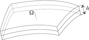
Let $\Omega$ be a two-dimensional smooth surface bounded by a smooth closed curve $\partial\Omega$. At each point of the surface $\Omega$ a segment of length $h$ in the direction perpendicular to the surface is drawn so that its center lies on the surface. If the length $h$ is sufficiently small, the segments do not intersect each other and fill the domain $\mathcal{V}$ occupied by a shell in its undeformed state shown schematically in Fig. 1, with $\Omega$ being the shell middle surface.

Thus, the undeformed shell occupies the domain specified by the equation

where $z^{i}=r^{i}(x^{\alpha})$ is the equation of the middle surface $\Omega$, and $n^{i}(x^{\alpha})$ are the cartesian components of the normal vector ${\bf n}$ to this surface. We shall use Latin indices, running from 1 to 3, to refer to the spatial co-ordinates and the Greek indices, running from 1 to 2, to refer to the surface co-ordinates $x^{1}$ and $x^{2}$. The curvilinear co-ordinates $x^{\alpha}$ take values in a domain of $\mathbb{R}^{2}$, while $x\in[-h/2,h/2]$. We analyze the forced vibration of the shell made of a functionally graded piezoelectric material. Let $\Omega_{\pm}$ denote the face surfaces of the shell corresponding to $x=\pm h/2$ in the above equation. We consider three methods of electrode arrangement encountered most often:

• (i)

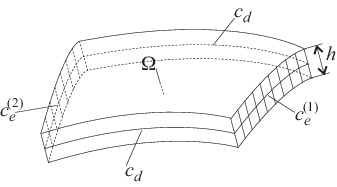
  There are no electrodes on the face surfaces of the shell (unelectroded face surfaces). The edge of the shell is partially electroded (see Figure 2).

  

  Thus, we assume that the contour $\partial\Omega$ is decomposed into open curves $c_{e}^{(1)},\ldots,c_{e}^{(n)}$ (where there are electrodes) and the remaining part $c_{d}$. For $x^{a}\in c_{e}^{(i)}\times[-h/2,h/2]$ on the electroded portions of the edge the electric potential is prescribed

  $$\varphi=\varphi_{(i)}(t),\quad i=1,\ldots,n.$$

  (10)

  On the unelectroded portion of the boundary the electric charge should vanish.

• (ii)

  The face surfaces $\Omega_{\pm}$ are fully coated by the electrodes. They form two equipotential surfaces where

  $$\varphi=\pm\varphi_{0}(t)/2,\quad\text{for $x=\pm h/2$}.$$

  (11)

  The difference between these values, $\varphi_{0}(t)$, is called voltage for short.

• (iii)

  The face surfaces of the shell are only partially coated by electrodes on $\mathcal{S}_{e\pm}\subset\Omega_{\pm}$. The remaining face surfaces $\mathcal{S}_{d\pm}$ are uncoated. This case can be regarded as the mixed situation of the two cases above.

For the asymptotic analysis of the FGP-shell inhomogeneous in the normal direction it is convenient to use the curvilinear coordinates $\{x^{\alpha},x\}$ introduced above and the co- and contravariant index notation for vectors and tensors, with Einstein’s summation convention being employed. In this coordinate system the action functional reads

where $\kappa=1-2Hx+Kx^{2}$ (with $H$ and $K$ being the mean and Gaussian curvature of the middle surface, respectively) and $da$ denotes the area element of the middle surface. The explicit dependence of the Lagrangian on the transverse coordinate $x$ of this functionally graded material is precisely indicated. The kinetic energy density becomes

where $a^{\alpha\beta}$ are the contravariant components of the surface metric tensor, while $w_{\alpha}$ and $w$ are the projections of the displacement vector onto the tangential and normal directions to the middle surface

The electric enthalpy density $W$ reads

The problem is to replace the three-dimensional action functional by an approximate two-dimensional action functional for a thin FGP-shell, whose functions depend only on the longitudinal co-ordinates $x^{1},x^{2}$ and time $t$. The possibility of reduction of the three- to the two-dimensional functional is related to the smallness of the ratios between the thickness $h$ and the characteristic radius of curvature $R$ of the shell middle surface and between $h$ and the characteristic scale of change of the electroelastic state in the longitudinal directions $l$ (see [29] and Section 5). We assume that

Additionally, we assume that

where $\tau$ is the characteristic scale of change of the functions $w_{i}$ and $\varphi$ in time (see [29]) and $c$ the minimal velocity of plane waves in the piezoelectric materials under consideration. This means that we consider in this paper only statics or low-frequency vibrations of the functionally graded piezoelectric shell. By using the variational-asymptotic method, the two-dimensional action functional will be constructed below in which terms of the order $h/R$ and $h/l$ are neglected as compared with unity (the first-order or “classical” approximation).

In order to fix the domain of the transverse co-ordinate in the passage to the limit $h\to 0$, we introduce the dimensionless co-ordinate

and transform the action functional to

Now $h$ enters the action functional explicitly through the components of the strain tensor $\varepsilon_{ab}$ and the electric field $E_{a}$

Here and below, the semicolon preceding Greek indices denotes the covariant derivatives on the surface, while the parentheses surrounding a pair of indices the symmetrization operation. Note that the raising or lowering of indices of surface tensors will be done with the surface metrics $a^{\alpha\beta}$ and $a_{\alpha\beta}$, $b_{\alpha\beta}$ and $c_{\alpha\beta}$ are the second and third fundamental forms of the surface, vertical bar followed by $\zeta$ indicates the partial derivative with respect to $\zeta$ and not with respect to $x^{\zeta}$.

Before applying the variational-asymptotic procedure to functional (13) let us transform the electric enthalpy density to another form more convenient for the asymptotic analysis [27]. We note that, among terms of $W(\varepsilon_{ab},E_{a})$, the derivatives $w_{\alpha|\zeta}/h$ and $w_{|\zeta}/h$ in $\varepsilon_{\alpha 3}$ and $\varepsilon_{33}$ as well as $E_{3}=-\varphi_{|\zeta}/h$ are the main ones in the asymptotic sense. Therefore it is convenient to single out the components $\varepsilon_{\alpha 3}$ and $\varepsilon_{33}$ as well as $E_{3}$ in the electric enthalpy density. We represent the latter as the sum of two quadratic forms $W_{\parallel}$ and $W_{\perp}$ corresponding to longitudinal and transverse electric enthalpy densities, respectively. These are defined by

Let us first find the decomposition (15) in the most general case of anisotropy [27]. Long, but otherwise simple calculations show that

where

Functions $c^{\alpha\beta\gamma\delta}_{N}(\zeta)$, $e^{\gamma\alpha\beta}_{N}(\zeta)$, $\epsilon^{\alpha\beta}_{N}(\zeta)$, $c^{3\alpha 3\beta}_{E}(\zeta)$, $c^{\alpha 333}_{E}(\zeta)$, $c^{3333}_{E}(\zeta)$, $\epsilon^{33}_{S}(\zeta)$, $e^{333}(\zeta)$, $e^{3\alpha 3}(\zeta)$, $r^{\alpha\beta}(\zeta)$, $r^{\alpha}(\zeta)$, $p_{\alpha}^{\mu\nu}(\zeta)$, $p_{\alpha}^{\mu}(\zeta)$, $q^{\alpha\beta}(\zeta)$, and $q^{\alpha}(\zeta)$ can be regarded as components of surface tensors referred to the basis vectors $\mathbf{t}_{\alpha}$ of the middle surface. We shall call them “two-dimensional” electroelastic moduli. They are evaluated in terms of the three-dimensional moduli by means of the formulas

where their dependence on the variable $\zeta$ is suppressed for short.

Note that, as these tensors are referred to the basis $\{\mathbf{t}_{\alpha},\mathbf{n}\}$, their components will depend on $\zeta$ through the shifter $\mu^{\beta}_{\alpha}=\delta^{\beta}_{\alpha}-h\zeta b^{\beta}_{\alpha}$ even for homogeneous shells. However, it can be shown for the FGP-shell inhomogeneous in the normal direction that components of two-dimensional electroelastic moduli of any rank, denoted symbolically by $A(\zeta)$, possess the property

where $A_{0}(\zeta)$ describe the physical inhomogeneity of the material and do not depend on the shifter (as in the case of FGP-plates with cartesian coordinates), while the factor $O(h/R)$ in the second term is due to the shifter $\mu^{\beta}_{\alpha}$ of the curvilinear coordinates solely. Therefore, when constructing 2-D shell theories having the error $h/R$ as compared with unity, it can be assumed that $A(\zeta)=A_{0}(\zeta)$.

Let us note certain special symmetry cases.

• 1.

  Mirror planes parallel to the middle surface. If properties of the piezoelectric material are invariant under reflections relative to planes parallel to the middle surface, then the following 2-D tensors vanish

  $$c^{\alpha 333}_{E}=0,\,e^{333}=0,\quad p^{\mu\nu}_{\alpha}=0,\,p^{\mu}_{\alpha}=0,\quad q^{\mu\nu}=0,\,q^{\mu}=0,$$

  and

  $$c^{\alpha\beta\gamma\delta}_{N}=c^{\alpha\beta\gamma\delta}_{P},\quad e^{\gamma\alpha\beta}_{N}=e^{\gamma\alpha\beta}_{P},\quad\varepsilon^{\alpha\beta}_{N}=\varepsilon^{\alpha\beta}_{P}.$$

• 2.

  n-fold rotation axes that coincide with the normal to the middle surface. When $n$ is even, all 2-D tensors of odd rank vanish

  $$e^{\gamma\alpha\beta}_{N}=0,\,c^{\alpha 333}_{E}=0,\,e^{3\alpha 3}=0,\,r^{\alpha}=0,\,p^{\mu\nu}_{\alpha}=0,\,q^{\mu}=0.$$

• 3.

  Transverse isotropy. When properties of the piezoelectric material are invariant under rotations about the normal to the middle surface (model of a piezoceramic shell polarized along the normal with symmetry $\infty\cdot m$), it can be shown that all 2-D tensors of odd rank vanish; the tensor $c^{\alpha\beta\gamma\delta}_{N}$ has the form

  $$c^{\alpha\beta\gamma\delta}_{N}=c^{N}_{1}a^{\alpha\beta}a^{\gamma\delta}+c^{N}_{2}(a^{\alpha\gamma}a^{\beta\delta}+a^{\alpha\delta}a^{\beta\gamma}),$$

  and all the 2-D tensors of second rank are spherical.

We restrict ourselves to the low frequency vibrations of the FGP-shell for which assumption (12) is valid. Based on this assumption we may neglect the kinetic energy density in the variational-asymptotic procedure.⁴⁴ 4 For the high-frequency vibrations of elastic and piezoelectric shells and rods where the kinetic energy density should be kept in the variational-asymptotic analysis see [5, 6, 23, 25, 26, 28, 29, 32]. Since there are two different cases of unelectroded and electroded faces of the shell, we shall do the asymptotic analysis for these cases separately.

References

• [1] Bailey, T., Ubbard, J., 1985. Distributed piezoelectric-polymer active vibration control of a cantilever beam. Journal of Guidance, Control, and Dynamics 8 (5), 605–611.
• [2] Berdichevsky, V. L., 1979. Variational-asymptotic method of constructing a theory of shells. Journal of Applied Mathematics and Mechanics 43 (4), 711–736.
• [3] Berdichevsky, V. L., 2010a. An asymptotic theory of sandwich plates. International Journal of Engineering Science 48 (3), 383–404.
• [4] Berdichevsky, V. L., 2010b. Nonlinear theory of hard-skin plates and shells. International Journal of Engineering Science 48 (3), 357–369.
• [5] Berdichevsky, V. L., Le, K. C., 1980. High-frequency long-wave shell vibration. Journal of Applied Mathematics and Mechanics 44 (4), 520–525.
• [6] Berdichevsky, V. L., Le, K. C., 1982. High frequency vibration of shells. Soviet Physics Doklady 27 (11), 988–990.
• [7] Berdichevsky, V. L., Misyura, V., 1992. Effect of accuracy loss in classical shell theory. Journal of Applied Mechanics 59 (2S), S217–S223.
• [8] Braides, A., 2002. Gamma-convergence for Beginners. Vol. 22. Clarendon Press.
• [9] Chen, W., Wang, L., Lu, Y., 2002. Free vibrations of functionally graded piezoceramic hollow spheres with radial polarization. Journal of Sound and Vibration 251 (1), 103–114.
• [10] Cheng, Z.-Q., Batra, R., 2000. Three-dimensional thermoelastic deformations of a functionally graded elliptic plate. Composites Part B: Engineering 31 (2), 97–106.
• [11] Crawley, E. F., De Luis, J., 1987. Use of piezoelectric actuators as elements of intelligent structures. AIAA journal 25 (10), 1373–1385.
• [12] Crawley, E. F., Lazarus, K. B., 1991. Induced strain actuation of isotropic and anisotropic plates. AIAA journal 29 (6), 944–951.
• [13] Dong, C., 2008. Three-dimensional free vibration analysis of functionally graded annular plates using the Chebyshev–Ritz method. Materials & Design 29 (8), 1518–1525.
• [14] Elishakoff, I., Pentaras, D., Gentilini, C., 2015. Mechanics of Functionally Graded Material Structures. World Scientific.
• [15] Friesecke, G., James, R. D., Müller, S., 2006. A hierarchy of plate models derived from nonlinear elasticity by gamma-convergence. Archive for Rational Mechanics and Analysis 180 (2), 183–236.
• [16] Han, X., Liu, G., Xi, Z., Lam, K., 2001. Transient waves in a functionally graded cylinder. International Journal of Solids and Structures 38 (17), 3021–3037.
• [17] He, X., Ng, T., Sivashanker, S., Liew, K., 2001. Active control of FGM plates with integrated piezoelectric sensors and actuators. International Journal of Solids and Structures 38 (9), 1641–1655.
• [18] Jha, D., Kant, T., Singh, R., 2013. A critical review of recent research on functionally graded plates. Composite Structures 96, 833–849.
• [19] Koiter, W. T., 1960. A consistent first approximation in the general theory of thin elastic shells. In: Proceedings of the IUTAM Symposium on the Theory of Thin Elastic Shells. North-Holland Amsterdam, pp. 12–33.
• [20] Koiter, W. T., 1970. On the mathematical foundation of shell theory. In: Proceedings of the International Congress on Mathematics Nice 1970. Vol. 3. pp. 123–130.
• [21] Koizumi, M., 1992. Recent progress of functionally gradient materials in Japan. In: 16th Annual Conference on Composites and Advanced Ceramic Materials I. Vol. 13. p. 333.
• [22] Le, K. C., 1979. On the static-geometric analogy. Bulletin of Moscow University, Math.-Mech. 34 (1), 70–76.
• [23] Le, K. C., 1982. High-frequency long-wave vibrations of piezoelectric ceramic plates. Soviet Physics Doklady 27 (5), 422–423.
• [24] Le, K. C., 1984. Fundamental relations of the theory of anisotropic piezoelectric shells. Bulletin of Moscow University, Math.-Mech. 39 (5), 57–60.
• [25] Le, K. C., 1985. High frequency vibrations of piezoelectric ceramic shells. Soviet Physics Doklady 30 (10), 899–900.
• [26] Le, K. C., 1986a. High frequency longitudinal vibrations of elastic rods. Journal of Applied Mathematics and Mechanics 50 (3), 335–341.
• [27] Le, K. C., 1986b. The theory of piezoelectric shells. Journal of Applied Mathematics and Mechanics 50 (1), 98–105.
• [28] Le, K. C., 1997. High frequency vibrations and wave propagation in elastic shells: variational-asymptotic approach. International Journal of Solids and Structures 34 (30), 3923–3939.
• [29] Le, K. C., 1999. Vibrations of shells and rods. Springer Verlag.
• [30] Le, K. C., Yi, J.-H., 2016. An asymptotically exact theory of smart sandwich shells. International Journal of Engineering Science.
• [31] Lee, C.-Y., Hodges, D. H., 2009a. Dynamic variational-asymptotic procedure for laminated composite shells - Part I: Low-frequency vibration analysis. Journal of Applied Mechanics 76 (1), 011002.
• [32] Lee, C.-Y., Hodges, D. H., 2009b. Dynamic variational-asymptotic procedure for laminated composite shells - Part II: High-frequency vibration analysis. Journal of Applied Mechanics 76 (1), 011003.
• [33] Leugering, G. R., Nazarov, S. A., Slutskij, A. S., 2012. Asymptotic analysis of 3D thin anisotropic plates with a piezoelectric patch. Mathematical Methods in the Applied Sciences 35 (6), 633–658.
• [34] Li, Q., Iu, V., Kou, K., 2008. Three-dimensional vibration analysis of functionally graded material sandwich plates. Journal of Sound and Vibration 311 (1), 498–515.
• [35] Liew, K. M., Zhao, X., Ferreira, A. J., 2011. A review of meshless methods for laminated and functionally graded plates and shells. Composite Structures 93 (8), 2031–2041.
• [36] Niino, M., Maeda, S., 1990. Recent development status of functionally gradient materials. ISIJ International 30 (9), 699–703.
• [37] Pan, E., Han, F., 2005. Exact solution for functionally graded and layered magneto-electro-elastic plates. International Journal of Engineering Science 43 (3), 321–339.
• [38] Prager, W., Synge, J. L., 1947. Approximations in elasticity based on the concept of function space. Quart. Appl. Math 5 (3), 241–269.
• [39] Preumont, A., 2002. Vibration Control of Active Structures: an Introduction. Kluwer Academic Publishers, Dordrecht.
• [40] Reddy, J., Wang, C., Kitipornchai, S., 1999. Axisymmetric bending of functionally graded circular and annular plates. European Journal of Mechanics-A/Solids 18 (2), 185–199.
• [41] Reddy, J. N., 2004. Mechanics of laminated composite plates and shells: theory and analysis. CRC press.
• [42] Roy, S., Yu, W., Han, D., 2007. An asymptotically correct classical model for smart beams. International Journal of Solids and Structures 44 (25), 8424–8439.
• [43] Sanders, J. L., 1959. An improved first order approximation theory of thin shells. In: NASA Report. Vol. 24.
• [44] Shen, H.-S., 2016. Functionally graded materials: nonlinear analysis of plates and shells. CRC press.
• [45] Tzou, H., Gadre, M., 1989. Theoretical analysis of a multi-layered thin shell coupled with piezoelectric shell actuators for distributed vibration controls. Journal of Sound and Vibration 132 (3), 433–450.
• [46] Vel, S. S., Batra, R., 2004. Three-dimensional exact solution for the vibration of functionally graded rectangular plates. Journal of Sound and Vibration 272 (3), 703–730.
• [47] Wen, P., Sladek, J., Sladek, V., 2011. Three-dimensional analysis of functionally graded plates. International Journal for Numerical Methods in Engineering 87 (10), 923–942.
• [48] Wu, C., Kahn, M., Moy, W., 1996. Piezoelectric ceramics with functional gradients: a new application in material design. Journal of the American Ceramic Society 79 (3), 809–812.
• [49] Wu, C.-P., Tsai, Y.-H., 2009. Cylindrical bending vibration of functionally graded piezoelectric shells using the method of perturbation. Journal of Engineering Mathematics 63 (1), 95–119.
• [50] Wu, X.-H., Chen, C., Shen, Y.-P., Tian, X.-G., 2002. A high order theory for functionally graded piezoelectric shells. International Journal of Solids and Structures 39 (20), 5325–5344.
• [51] Yiqi, M., Yiming, F., 2010. Nonlinear dynamic response and active vibration control for piezoelectric functionally graded plate. Journal of Sound and Vibration 329 (11), 2015–2028.
• [52] Zhong, Z., Shang, E., 2003. Three-dimensional exact analysis of a simply supported functionally gradient piezoelectric plate. International Journal of Solids and Structures 40 (20), 5335–5352.