The kinematic formula in the 3D-Heisenberg group
Abstract.
By studying the group of rigid motions, , in the 3D-Heisenberg group , we define the density and the measure for the sets of horizontal lines. We show that the volume of a convex domain is equal to the integral of length of chord over all horizontal lines intersecting . As the classical result in integral geometry, we also define the kinematic density for and show the probability of randomly throwing a vector interesting the convex domain under the condition that is contained in . Both results show the relationship connecting the geometric probability and the natural geometric quantity in [9] approached by the variational method.
1. Introduction
We adapt the methods of integral geometry to study the 3D-Heisenberg group which is a non-compact CR manifold with zero Tanaka-Webster torsion and zero Tanaka-Webster curvature. After the brief history of integral geometry and the introduction of CR geometry, we will illustrate how our formulas show the relationship connecting these fields.
The roots of integral geometry may date back from geometric probability and the study of invariant measures by integration techniques, which consider the probability of random geometric objects interacting to each other under a group of transformations, for example, Buffon’s needle problem and Bertrand’s paradox. In the late nineteenth and early twentieth century, a variety of problems in geometric probability arose and lead to systematical studies in this field. Works of Crofton, Poincaré, Sylvester and others build up the foundation of integral geometry. A series of articles related to the developments of geometric probability in this age was elaborated by Maran [20, 21], Little [18], and Baddeley [1]. When the concept of invariant measure had became clear, Wilhelm Blaschke [3] and his school initiated integral geometry. Santaló’s book [24] has been one of the most important books on the subject; Howard’s book [16] deals with the cases in Riemannian geometry; Zhou [32, 33] derives several integral formulas for submanifolds in Riemannian homogeneous spaces; The book of Schneider and Weil [25] includes the fundamental knowledge of integral geometry and recent development of integral and stochastic geometry. Due to page restriction, we refer the delicate surveys [30] [31].
CR geometry studies the geometry of the boundary of a smooth strictly pseudo-convex domain in , and then develops to the abstract CR manifolds. The foundational work was built by Chern-Moser [8] in 1974, and a closely connected work is given by Webster [27] and Tanaka [26] independently; they introduced the pseudohermitian geometry where a connection is given associated to a choice of a contact form and curvature invariants. We point out that the relationship between CR geometry and pseudohermitian geometry have the strong analogy to that between conformal geometry and Riemannian geometry [2]. The introductory surveys, emphasizing recent development of three dimensional pseudohermitian geometry, can be found in [29, 28].
Next we give the background of our studying target. The 3D-Heisenberg group is the Euclidean space with a group multiplication (see Section 2). A rigid motion (called a pseudohermitian transformation) in is a diffeomorphism defined on preserving the CR structure and the contact form , namely,
Denote the group of pseudohermitians by . Similar to the usual group of translations in , in [14] we show that consists of left-translations and rotations , (as shown (2.3)). The understanding of the structure of plays the important role when using the method of moving frames (see equations (2.3)(3). Let be an embedded surface in and denote the set of points on where the contact plane is tangent to the tangent plane of the surface. Given an orthonormal basis defined on w.r.t. the Levi metric, where on and , and is the Reeb vector field. Suppose is the dual basis of . To our purpose, two geometric quantities naturally following the geometry in should be introduced
| (1.1) | ||||
| (1.2) |
which are called, respectively, the volume of the domain and the p-Area of its boundary . The authors in [9] show that the volume actually is the Lebesque volume in , while the p-area form , resulted from the variation of volume along the Legendrian normal , is globally defined on and vanishes on . The similar notions of volume and area are also studied by [22, 23, 15, 5] when considering the -surface enclosing a bounded set ; the area of coincides with the -perimeter of of . The authors adapt the usual normal vector perpendicular to the surface, while we consider the Legendrian normal which later on develops toward to the studies of umbilic hypersurfaces in higher dimensional Heisenberg Group , see [11].
A horizontal line is a straight line in such that its velocity vector is always tangent to the contact plane. In the next section, we shall show that every horizontal line can be uniquely represented, up to an orientation, by three parameters (equivalently, by the base point ). Denote by and therefore the three-form is invariant under (see (3.8)). Follow the classical integral geometry [24][7], we give the analogous definition of measure for a set of horizontal lines.
Definition 1.
The measure of a set of horizontal lines is defined by the integral over the set ,
where the diffeerential form is called the density for sets of horizontal lines.
Remark that up to a constant factor, this density is the only one that is invariant under motions of . In convention, the density will always be taken at absolute value.
Recall that the Crofton’s formula: for a convex domain in with the length of boundary , we have ([24], Chapter 4.2)
By using the method of moving frame for the convex domain with boundary , we show the Crofton-type formula ([14] Theorem 1.11)
| (1.3) |
Also, in the Euclidean plane ([24], Chapter 3), it shows that the area of a convex domain is equal to the integral of length of chord over all lines intersecting ,
where stands for the line in , is the density of set of lines. Our first main result is the analogy in :
Theorem 1.
Let be a convex domain with boundary in . Suppose is an oriented horizontal line intersecting with by the length of chord w.r.t. the Levi metric. Then
where is the density of the horizontal lines and is the Lebesque volume of in .
Once we have defined the measure of sets of lines, the probability ([24], Chapter 2) that a random line is in the set when it is known to be in the bigger set containing can be defined by the quotient of the measures
| (1.4) |
Thsu, by the conditional probability and (1.3), we immediately have the corollaries:
Corollary 1.1.
Given a convex 3-domain in with boundary , and randomly throw an oriented horizontal line interesting once a time with chord length . The average chord length of the lines interesting is
Because of the Lie group structure of , we can define the the moving frame at the point by moving the standard frame (defined in (2.1)) at the original along the horizontal line under translations in (see Section 2). Note that for any . There exists an one-to-one correspondence associated to and the moving frames, and thus any element in is uniquely parametrized by four variables , where the point dominates the position of the frame, the rotation on . Moreove, we shall show the following four-form is invariant under , and hence one defines it as the kinematic density of .
Definition 2.
The invariant -form
| (1.5) |
is called the kinematic density for the group of motions in , where is the angle from the standard vector to the frame vector , .
We shall also show that the invariant volume element of has the other expression
| (1.6) |
where is the oriented distance from the base point to w.r.t. the Levi-metric, the density in Definition 1.
By integrating over a domain in , one gets the measure of the corresponding set of motions (as [24], called the kinematic measure). This kinematic measure is actually somewhat a unexpected geometric quantity, p-Area, so it is worth to believe that the suitable approach can help us understand CR (pseudohermitian) geometry from the viewpoint of integral geometry. The following result gives an evidence of the connections between these two fields.
Theorem 2.
Given a convex 3-domain in with boundary . Randomly throw an oriented line segment (may not be necessarily horizontal) with length w.r.t. the Levi metric (Fingure 1). The measure of random line segments intersecting the domain is
| (1.7) |
where is the kinematic density, the Lebseque volume of , and p-Area() the p-area of the surface .
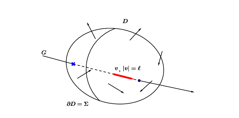
Remark 1.
We take for granted that in the sense of or . When restricted our attention to only, the equation becomes
and the measure of is
With the measure, we immediately have the probability of containment problem.
Corollary 1.2.
Let be convex 3-domains with boundary for , such that . The probability of randomly throwing a vector with length w.r.t. Levi metric in intersecting is
Acknowledgment. Part of the contents in this article was completed during the author’s postdoctoral at National Central University, Taiwan. I would like to thank my mentor, Prof. Hung-Lin Chiu, for his introduction and inspiration to this problem.
2. Preliminary
For basic knowledge of the Heisenberg group, we refer [9](appendix), [22], and our previous work [14]; also, [10, 28, 29]. There are some works from sub-Riemannian approaches, e.g. [4, 22, 6, 17, 23, 5, 15]. The three dimensional Heisenberg group is , as a set, together with the group multiplication (left-invariant translation)
is a 3-dimensional Lie group. Any left invariant vector field, at point , is a linear combination of the following standard vector fields:
| (2.1) | ||||
| (2.2) |
The standard contact structure } on is the subbundle of the tangent bundle ; equivalently, we can also define to be the kernal of the standard contact form
The standard CR structure on is the almost complex structure defined on such that
On a natural metric
called the Levi metric, ; for we define the length of by .
In our previous work [14], we show that any pseudo-hermitian transformation can be represented by a left-invariant translation for and a rotation . There exits the one-to-one correspondence between the group actions and the matrix multiplication
| (2.3) |
Let be a smooth hypersurface in . Recall that a point is called singular if the contact plane conincides with the tangent plane at , namely, ; otherwise is called regular. Denote is the set of singular points. It is easy to see that is a closed set. At each regular point , there exists (unique up to a sign) a vector , which defines a one dimensional foliation consisting of integral curves of and we call it the characteristic curves. The vector perpendicular to , in the sense of Levi-metric, is called Legendrian normal or Gauss map [9]. Let be a smooth domain with boundary and be the dual basis of where is the Reeb vector field such that and . Cheng-Hwang-Malchiodi-Yang [9] study the minimal surface in via the variational approach and define the volume and the p-Area respectively
| (2.4) | ||||
| (2.5) |
We point out that is a normalization constant and this volume is just the usual Euclidean volume. While p-Area comes from a variation of the surface in the normal direction for some suitable function with compact support on the regular points of . Note that we can continuously extend over the singular set such that it vanishes on . Thus, p-Area is globally defined on . In the same paper, the authors also define the p-mean curvature and of associated p-minimal surfaces; Malchiodi [19] summarize the other two equivalent definitions for the p-mean curvature.
3. Invariants for sets of horizontal lines
In the section, we will derive the invariants for the set of horizontal lines as shown in Definition 3.8 and the other expression of the kinematic density for .
Given a regular curve . Its velocity can always be decomposed into the part tangent to the contact plane and the other orthogonal to w.r.t the Levi metric, namely,
A horizontally regular curve is a regular curve with non-zero contact part
In [14] (Proposition 4.1) the authors show that any horizontally regular curve can be parametrized by the horizontal arc-length such that . Throughout the article, we always assume that the curve (or line) is parametrized under this condition. Moreover, if is a curve joining points and , we have the distance
| (3.1) |
Now we characterize the horizontal lines. A horizontal line in is uniquely determined by three parameters : the angle of its projection onto -plane from the positive -axis to the line perpendicular to , the distance from the origin to the footpoint , and the hight of base point by lifting of to . (as Figure 2.)

Use (2.1), the curve can be parametrized by the base point and the unit vector
| (3.2) |
(3.2) implies that the points on satisfy the conditions
Therefore, we have the following expression for any horizontal line
Suppose the horizonal line is obtained by transformed under a pseudohermition transformation . By the matrix multiplication (2.3), it is easy to calculate the transformed line satisfying
and therefore
| (3.8) |
To the end, the 3-form is invariant under . Moreover, if the measure of a set of horizontal lines is defined by any integral of the form
| (3.9) |
for some function . Follow the spirit of classical integral geometry and geometric probability, the most natural measure is to be invariant under the group of rigid motion in . If we want the measure to equal the measure of transformed set for any set and any motion, by , the function has to be constant. Choose the constant to be unity one gets the Definition 1.
Next we derive the alternative expression of the kinematic density (1.6. Let be the moving frame obtained from the standard frame at the original by the left-invariant translation to the point and the angle that makes with the standard vector (as Figure 3).

We observe that and the angle indicates the rotation of the frame vector from the vector on the contact plane . Denote the oriented distance
w.r.t. the Levi metric, the sign depends on the direction and the orientation of . Since
we have
Take the derivatives and make the wedge product all together, we reach the other expression (1.6) of the kinematic density for the group of motions in
| (3.10) |
which is indeed invariant under by .
4. Proof of Theorem 1
We shall prove the lemma first. Given a horizontal line and two points , on . Since is horizontal, . If we consider the distance joining and defined as (3.1), the infinitesimal length varies by the Levi-metric defined on different contact plane for all points between and ; while by considering , we define the other distance
| (4.1) |
where the infinitesimal length depends only on the contact plane of the initial point . However, the lemma below shows that both distances are exactly same.
Lemma 4.1.
Given an oriented horizontal line , parametrized by horizontal arc-length , passing through the points to . Then two distances defined by and are same, .
Proof.
Note that since is horizontal, and . Thus, the distance . Therefore, we can always regard any point between between and being parametrized as the end of the vector ejecting from by . Clearly, its tangent is a unit vector on for any , so and the result follows immediately.
Now we prove Theorem 1.
Proof.
First we observe that the slope of projection of on -plane is , which is independent of the orientation of . Now fixed a pair of and consider the cross-section of domain and the vertical plane along the projection
Since the projection onto -plane again is , we may set the first two coordinates of points on satisfying
Thus, for or , the plane can be parametrized by
for some interval , depending the range of domain , where
| (4.2) | ||||
Now we use the following Lemma.
Lemma 4.2 ([14] Lemma 8.7).
Let be the tangent vector field defined on the regular surface in . Then the vector is also on the contact bundle (and hence in ) if and only if pointwisely the coefficients and satisfy
| (4.3) |
Since is an one-dimensional foliation (a horizontal line in this case) restricted on , is a linear combination of and . By Lemma 4.2, we choose and which satisfy . Use (4.2), we have
| (4.4) |
| (4.5) | ||||
When or , the horizontal lines lie on the planes parallel to the -plane, and therefore , which implies the density
| (4.6) |
Finally, combine both cases ,
where we use the fact that is Lebesque volume form in in the last identity, and complete the proof.
Remark: if consists of finitely many simply-connected subsets, then the right-hand-side of (1) becomes the sum of volumes for each subset.
5. Proof of Theorem 2
Proof.
Give a fixed line segment outside of the boundary . There exists an horizontal line along the vector penetrating at two points. Now move in the direction of from outside of until the end of leaving . The condition gives the distance that the end of the vector traveling over , so by Theorem 1 and (1.3) we have
References
- [1] A. Baddeley, A Fourth Note on Recent Research in Geometrical Probability, Adv. in Appl. Probability, Vol. 9, No. 4 (1977), pp. 824-860.
- [2] M. Beals, C. Fefferman, R. Grossman, Strictly Pseudoconvex Domains in , Bull. Amer. Math. Soc. (N.S.) V(8), No.2, (1983), 125-322.
- [3] W. Blaschke, Integralgeometrie 2:Zu Ergebnissen von M. W. Crofton, Bull. Math. Soc. Roumaine Sci., 37, 1935, 3-7.
- [4] O. Calin, D.C. Chang, P. Greiner, Geometric Analysis on the Heisenberg Group and Its Generalizations, AMS Studies in Adv. Math., 40, 2007.
- [5] L. Capogna, D. Danielli, N. Garofalo, An isoperimetric inequality and the geometric Sobolev embedding for vector fields, Math. Res. Lett. 1 (2), (1994), 203-215.
- [6] , L. Capogna, D. Danielli, S.D. Pauls, J. Tyson, An Introduction to the Heisenberg Group and the Sub-Riemannian Isoperimetric Problem, Progress in Mathematics, 2007.
- [7] S.S. Chern, Lectures on integral geometry, notes by Hsiao, H.C., Academia Sinica, National Taiwan University and National Tsinghua University, (1965).
- [8] S.S. Chern, J.K. Moser, Real Hyperserufaces in Complex Manifolds, Acta Math. 133, (1974), 219-271.
- [9] J.H.Cheng, J.F.Hwang, A.Malchiodi, P.Yang, Minimal surfaces in pseudohermitian geometry, Ann. Scuola Norm. Sup. Pisa Cl. Sci. (5), Vol. IV(2005), 129-177.
- [10] J.H. Cheng, J.F. Hwang, A. Malchiodi, P. Yang, A Codazzi-like equation and the singular set for smooth surfaces in the Heisenberg group, J. Reine Angew. Math., 671, (2012), 131–198.
- [11] J.H. Cheng, H.L. Chiu, J.F. Hwang, P. Yang, Umbilic hypersurfaces of constant sigma-k curvature in the Heisenberg group, Calc. Var. Partial Differential Equations 55 (2016), no. 3, Art.66, 25 pages.
- [12] J.H. Cheng, J.F. Hwang, P. Yang, Regularity of smooth surfaces with prescribed p-mean curvature in the Heisenberg group, Math. Ann., 344, (2009), no. 1, 1–35.
- [13] J.H. Cheng, J.F. Hwang, P. Yang, Existence and uniqueness for p-area minimizers in the Heisenberg group, Math. Ann., 337, (2007), no. 2, 253–293.
- [14] H.L.Chiu, Y.C. Huang, S.H.Lai, The application of the moving frame method to Integral Geometry in Heisenberg group, Preprint, http://arxiv.org/abs/1509.00950.
- [15] , B. Franchi, R. Serapoioni, F. S. Cassano, Rectifiability and perimeter in the Heisenberg group, Math. Ann. 321 (3), (2001), 479-531.
- [16] R. Howard, The Kinematic Formula in Riemannian Homogeneous Spaces, Mem. Amer. Math. Soc. No. 509, V106, 1993.
- [17] G.P. Leonardi, S. Masnou, On the isoperimetric problem in the Heisenberg group , Annali di Matematica Pura ed Applicata, V184,4, (2005), pp 533-553.
- [18] D.V. Little, A Third Note on Recent Research in Geometrical Probability, Adv. in Appl. Probability, Vol. 6, No. 1 (1974), pp. 103-130.
- [19] A. Malchiodi, Minimal surfaces in three dimensional pseudo-hermitian manifolds, Lect. Notes Semin. Interdiscip. Mat., 6, Semin. Interdiscip. Mat. (S.I.M.), Potenza, 2007.
- [20] P.A.P. Moran, A Note on Recent Research in Geometrical Probability, J. of Appl. Probability, Vol. 3, No. 2 (1966), pp. 453-463.
- [21] P.A.P. Moran, A Second Note on Recent Research in Geometrical Probability, Adv. in Appl. Probability, Vol. 1, No. 1 (1969), pp. 73-89.
- [22] M.Ritoré, C. Rosales, Area-stationary surfaces in the Heisenberg group , Adv. in Math., 219 (2008), pp.633-671.
- [23] M. Ritoré, C. Rosales, Rotationally invariant hypersurfaces with constant mean curvature in the Heisenberg group , J. Geom. Anal., 16(4), (2006), 703-720.
- [24] L. A. Santaló, Integral Geometry and Geometric Probability, Cambridge Mathematical Library, 2nd edition, 2004.
- [25] R.Schneider, W. Weil, Stochastic and Integral Geometry, Springer, 2008.
- [26] N. Tanaka, A differential geometric study on strongly pseudo-convex manifolds, Khokuniya, Yokyo, 1975.
- [27] S. Webster, Pseudo-hermitian structures of a real hyper-surfaces, J. Diff. Geo., 13(1978), 25-41.
- [28] P. Yang, Minimal Surfaces in CR geometry, Geometric analysis and PDEs, 253–273, Lecture Notes in Math., 1977, Springer, 2009,
- [29] P. Yang, Pseudo-Hermitian Geometry in 3-D, Milan J. Math. V(79), (2011), 181-191.
- [30] G.Y. Zhang, A lecture on Integral Geometry, Proceedings of the fourteenth Internatioanl Workshop on Diff. Geom. 14(2010), 13-30.
- [31] J.Z. Zhou, Kinematic formulas in Riemannian spaces, Proceedings of the tenth Internatioanl Workshop on Diff. Geom. 10(2006), 39-55.
- [32] J.Z. Zhou, Kinematic Formulas for Mean Curvature Powers of Hypersurfaces and Hadwiger’s Theorem in , Trans. Amer. Math. Soci., v345, No1, 1994, pp. 243-262.
- [33] J.Z. Zhou, M. Li, Kinematic Formulas of Total Mean Curvatures for Hypersurfaces, Chinese Ann. Math. 37B(1), 2016, 137–148.