Explicit Solutions for Optimal Stopping of Linear Diffusion
and Its MaximumThanks: First Draft: September 28, 2015. This version: March 31, 2016. This work is in part supported
by Grant-in-Aid for Scientific Research (B) No. 26285069, Japan Society for the Promotion of Science.
Abstract.
We provide, in a general setting, explicit solutions for optimal stopping problems that involve diffusion process and its running maximum. Our approach is to use the excursion theory for Lévy processes. Since general diffusions are, in particular, not of independent increments, we use an appropriate measure change to make the process have that property. Then we rewrite the original two-dimensional problem as an infinite number of one-dimensional ones and complete the solution. We show general solution methods with explicit value functions and corresponding optimal strategies, illustrating them by some examples.
Key words: Optimal stopping; excursion theory;
diffusions.
Mathematics Subject Classification (2010) : Primary: 60G40
Secondary: 60J75
1. Introduction
We let be one-dimensional diffusion and denote by the reflected process,
where with . Hence is the excursion of from its running maximum . We consider an optimal stopping problem that involves both and . It is subject to absorbing boundary that varies with . That is,
| (1.1) |
where the rewards and are measurable functions from to and is also a measurable function. The rigorous mathematical definition of this problem is presented in Section 2. In this paper, we shall solve for optimal strategy and corresponding value function along with optimal stopping region in the -plane.
For optimal stopping that involve both and , we mention a pioneering work of Peskir [14] where the author used the “maximum principle”. There are also Ott [13] and Guo and Zervos [10]. In the former paper, the author solves problems including a capped version of the Shepp-Shiryaev problem (the Russian option) [18]. The latter makes another contribution that extends [18] and the reward function therein is with . This reward function includes perpetual call, lookback option, etc. as special cases. In many solved problems, Brownian motion or geometric Browninan motion is used as underlying process in an effort to obtain tractable solutions. A recent development in this area includes Alvarez and Matoäki [2] where a discretized approach is taken to find optimal solutions and a corresponding numerical algorithm is presented.
The idea of our solution method is the following: we look at excursions that occur from each level of , during an excursion from level , the value of is fixed until returns to . Using this, the problems reduce to an infinite number of one-dimensional optimal stopping problems. In this spirit, we then attempt to rewrite the problem equation (1.1) in the form of sequences of excursions. For finding the explicit form of the value function, we employ the theory of excursion of Lévy processes, in particular the characteristic measure that is related to the height of excursions. (Refer to Bertoin [4] as a general reference.) Since the diffusion is not in general of independent increments, we use the measure change (3.3) to make the diffusion behave like a Brownian motion under the new measure. Having done that, we solve, at each level of , one-dimensional optimal stopping problems by using the excessive characterization of the value function. This corresponds to the concavity of the value function after certain transformation. We briefly review this transformation in Section 2.2. See Dynkin[9], Alvarz[1] and Dayanik and Karatzas [7] for more details. For the excursion theory for spectrally negative Lévy processes (that have only downward jumps), we mention Avram et al. [3], Pistorius [16] [17] and Doney [8] where, among others, an exit problem of the reflected process is studied.
Our contributions in this paper may advance the literature in several respects: we do not assume any specific forms or properties in the reward functions (except for mild ones), and we provide explicit forms of the value function and illustrate the procedure of the solution method. In contrast to the literature, our approach is rather direct, without resorting to the variational inequality. See Section 3. Accordingly, the solution method can be applied in a more general setting.
The rest of the paper is organized as follows. In Section 2, we formulate a mathematical model with a review of some important facts of linear diffusions, and then find an optimal solution. The key step is to represent and compute the value , which is handled in Sections 3 and 4. Under the mild assumptions (Assumption 4.1), we present in an explicit form. The next step is to find in Section 5. Moreover, we shall demonstrate the methodology by using a new problem (Section 5.1) as well as some problems in the literature (Section 4.3.1 and 4.3.2). Let us stress that the new problem might not be easily handled by the conventional methods. Appendices include a proof of the technical lemma and some discussion about the smooth-fit principle in this problem.
2. Mathematical Model
Let the diffusion process represent the state variable defined on the probability space , where is the set of all possible realizations of the stochastic economy, and is a probability measure defined on . The state space of is given by , where and are natural boundaries. That is, cannot start from and exit from or . We denote by the filtration with respect to which is adapted and with the usual conditions being satisfied. We assume that satisfies the following stochastic differential equation:
where for any and is a standard Brownian motion.
The running maximum process with is defined by . In addition, we write for the reflected process defined by . We consider the following optimal stopping problem and the value function associated with initial values and ;
| (2.1) |
where and is the expectation operator corresponding to , is the constant discount rate and is the set of all -adapted stopping times. The payoff is composed of two parts; the running income to be received continuously until stopped, and the terminal reward part. The running income function is a measurable function that satisfies
The reward function is assumed to be measurable. Our main purpose is to calculate and to find the stopping time which attains the supremum.
For each collection of Borel measurable sets, we define a stopping time by
| (2.2) |
and define a set of stopping times by . In other words, is the first time the excursion from level, say , enters the region . Suppose that for any , we write
2.1. Optimal Strategy
We will reduce the problem (2.1) to an infinite number of one-dimensional optimal stopping problem and discuss the optimality of the proposed strategy (2.2). Let us denote by the -potential of :
From the strong Markov property of , we have
| (2.3) | |||||
Hence the value function can be written as
where
| (2.4) |
Since has nothing to do with the choice of , we concentrate on .
Let us first define the first passage times of :
By the dynamic programming principle, we can write as
| (2.5) |
for any stopping time . See, for example, Pham [15] page 97. Now we set in (2.5). For each level from which an excursion occurs, the value does not change during the excursion. Hence, during the first excursion interval from , we have for any , and (2.5) can be written as the following one-dimensional problem for the state process ;
Now we can look at only the process and find .
In relation to (2.1), we consider the following one-dimensional optimal stopping problem as for and its value function ;
| (2.6) |
where is a constant. Note that holds when , and we shall present how to characterize and compute in Sections 3 and 4.
Recall that, in pursuit of optimal strategy in the linear diffusion case, we can utilize the full characterization of the value function and optimal stopping rule. In particular, an optimal stopping is, in a very general setup, attained by the threshold strategy. That is, one should stop when at the first time that enters a certain region, called stopping region. See Dayanik and Karatzas [7]; Propositions 5.7 and 5.14. See also Pham [15]; Section 5.2.3. Note that, however, writing the value of in an explicit form is not trivial and is an essential part of the solution, which we shall do in the next section (see Propositions 3.1 and 4.1).
2.2. Important Facts of Diffusions
Let us recall the fundamental facts about one-dimensional diffusions; let the differential operator be the infinitesimal generator of the process defined by
and consider the ODE . This equation has two fundamental solutions: and . We set to be the increasing and to be the decreasing solution. They are linearly independent positive solutions and uniquely determined up to multiplication. It is well known that
| (2.7) |
For the complete characterization of and , refer to Itô and McKean [11]. Let us now define
| (2.8) |
Then is continuous and strictly increasing. Next, following Dynkin (pp. 238, [9]), we define concavity of a function with respect as follows: A real-valued function is called -concave on if, for every ,
Now consider the optimal stopping problem:
where : . Let be the smallest nonnegative concave majorant of
| (2.9) |
where is the inverse of . Then we have and the optimal stopping region is
as in Propositions 4.3 and 4.4 of [7]. Note that for the rest of this article, the term “transformation” should be understood as (2.9).
When both boundaries and are natural, for all if and only if
| (2.10) |
are both finite.
3. Representation of
Now we look to an explicit solution of for . The first step is to find in (2.1). That it, we consider the case . Set stopping times as and define the function by
| (3.1) |
for which . Since optimal strategy belongs to threshold strategies, we shall focus on the set of in (2.2). In other words, if , given a threshold strategy where is in the form of , the value is equal to . Accordingly, on the set .
From the strong Markov property of , when and , we have
| (3.2) | |||||
Now we calculate these expectations by changing probability measure. We introduce the probability measure defined by
| (3.3) |
Then is a process in natural scale under this measure . See Borodin and Salminen [5](pp. 33) and Dayanik and Karatzas [7] for detailed explanations. Hence we can write, under , , where is a constant and is a Brownian motion under . Since is a Lévy process, we can define the process of the height of the excursion as
and otherwise, where . Then is a Poisson point process, and we denote its characteristic measure under by of . It is well known that
See, for example, Çinlar [6] (pp. 416). By using these notations, we have11 1 Note that when the diffusion is a standard Brownian motion , then and the right-hand side reduces to .
| (3.4) | |||||
On the other hand, from the definition of the measure , we have
Combining these two things together,
| (3.5) |
Similarly, by changing the measure and noting that , we have
| (3.6) | |||||
Since is a Lévy process under , we can apply Theorem 2 in Pistorius [17] to calculate the last probability. Then we have
| (3.7) |
We have, up to this point, proved the following:
Proposition 3.1.
When , the function for can be represented by
| (3.8) | |||||
This representation of applies to general cases.
4. Computing
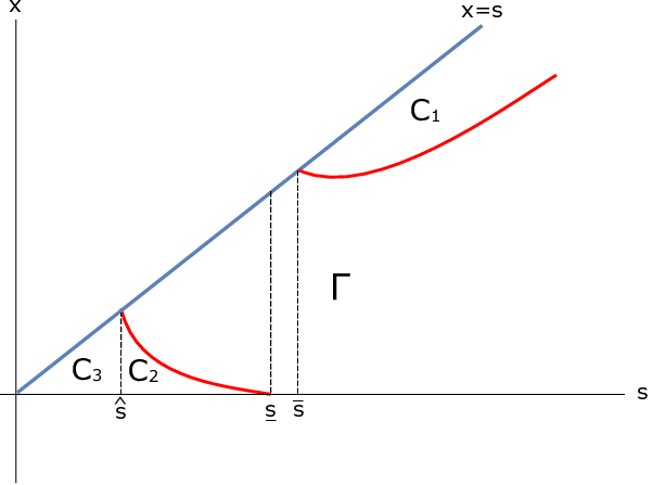
In solving an optimal stopping problem involving and , one of the aims is to draw a diagram like Figure 3. Note that we draw the diagram with on the horizontal axis since it is better understood than otherwise. For distinct values in the -diagram, we need to determine whether a point in is in the continuation region () or stopping region (). The task in this subsection22 2 Once this is done, then the next task is to examine the points by moving downwards to from the diagonal . We take this in Section 5 and solve an example in 5.1. is to compute the value at a point on the diagonal and to determine whether it belongs to or .
As stressed before, once we fix , the problem reduces to one-dimensional problems in and hence the way to find is similar to the one described in Section 2.2. Specifically, we set and attempt to find the smallest nonnegative concave majorant of
| (4.1) |
in the neighborhood of . Let us denote by (resp. ) the stopping region (resp. continuation region) with respect to the reward in (4.1), corresponding to this . Note that this (resp. ) should be distinguished from the stopping region (resp. ) of the problem (2.1), the final object to figure out. Due to the dependence of the reward on , however, there are some situations where we need to be careful. To discuss, we shall hereafter (for the rest of this section) assume the following:
Assumption 4.1.
Denote by the threshold point that separates and with respect to the reward associated with this .
- (i)
is increasing in ,
- (ii)
for , the continuation region corresponding to is in the form of or , and
- (iii)
(2.10) holds.
The first assumption is merely to restrict our problems to practical ones because we are solving maximization problems. The second is to make our argument concrete and simplistic. More complicated structure can be handled by some combinations of the cases prescribed below. For the third, since our main concern is to find a finite value function, we shall consider the case where (2.10) holds.
4.1. Case (1):
If belongs to , we have ; however, instead of stopping immediately, there is a possibility that a greater value can be attained if one stops during the excursion from some upper level . Recall that Proposition 3.1 has incorporated this. See also Remark 4.2 below. Now we wish to obtain more explicit formulae for from the general representation (3.8). For this purpose, let us denote
to avoid the long expression and rewrite (3.8) in the following way: for any ,
This expression naturally motivates us to set as
| (4.2) |
and we have . Dividing both sides by and choosing the optimal level , we have, for any given,
| (4.3) |
Let us consider the transformation of a Borel function defined on through
| (4.4) |
on where is the inverse of the strictly increasing in (2.8). If we evaluate at , we obtain , which is the form that appears in (4.3). Note that
| (4.5) |
Proposition 4.1.
Fix . If (1) the reward function is increasing in the second argument and (2) if is strictly convex on , we have
| (4.6) |
where
and is the maximizer of the map
If (2)’ is linear on , then is to be replaced by
Remark 4.1.
The strict convexity of implies
| (4.7) |
On the other hand, if is linear, then the inequality in (4.7) is replaced by the equality:
| (4.8) |
We shall use this property in the proof of Lemma 4.1. Note that it is easily proved that geometric Brownian motion satisfies (4.7) and Brownian motion (with or without drift) does the other one. The functions of Orstein-Uhlenbeck process (with and ) and its exponential version (where are positive constant) involve special functions; the parabolic cylinder function and the confluent hypergeometric function of the second kind, respectively (see Lebedev [12]). While it is hard to prove the log convexity of these special functions, it is numerically confirmed that both processes satisfy (4.7). Moreover, the equality condition (4.8) implies that so that is an exponential function. Hence it is confirmed that this case includes Brownian motion.
Proof.
(of Proposition 4.1) Let us first take the strictly convex case of . For taking limits of in (4.2), we need the following lemma whose proof is postponed to Appendix A:
Lemma 4.1.
Under the assumption of Proposition 4.1 with convex , for sufficiently close to zero, we have
| (4.9) |
Note that for all and and that for all .
Suppose that the lemma is proved, let us continue the proof of Proposition 4.1. By using (4.9) in Lemma 4.1, we can write, for small,
| (4.10) |
Moreover, since , the optimal threshold should satisfy
from which equation, in view of (4.10), we obtain
where the last equality is obtained by L’Hôpital’s rule, and hence is the value which gives the supremum to .
When is linear, in lieu of (4.9), we claim that
| (4.11) |
for sufficiently small. The intuition here is the following: since in Lemma 4.1 can be written as (as ) and in case of Brownian motion, , the factor should be independent of . It can be easily seen that the proof of Lemma 4.1 holds in this case, too. Accordingly, instead of (4.2), we have
For the rest, we just proceed as in the proof of Proposition 4.1 to obtain . ∎
Remark 4.2.
Let us slightly abuse the notation by writing to avoid the long expression. Note that is the value corresponding to the strategy with and for every ; that is, this amount is obtained when we stop if goes below in the excursion at level and behave optimally at all the higher levels .
In summary, in Case (1), we should resort to Proposition 4.1 to compute . If for this , we shall have .
4.2. Case (2):
4.3. Case (3):
is defined in Assumption 4.1. For this case, the typical situation is that is monotonically decreasing in . See Figure 3. The curve separating the region and corresponds to the function . Then define the point such that
holds. One receives when stops there. In contrast to the previous Cases (1) and (2), is located to the left of , we are not supposed to stop during the excursions from the level . Mathematically, it means that we let in (3.8) of Proposition 3.1. The left boundary is assumed to be natural and hence and , the Dirac measure sitting at . Now, from (3.7), (3.8) simplifies to
| (4.12) |
which is, in view of (2.7), simply the expected discounted value of . Note that for , the reward does not depend on and thereby
with respect to this reward, for .
Before moving on to find the general solution , it should be beneficial to briefly review some special cases in finding . In this section, the diffusion is geometric Brownian motion and provides and with and . The parameters are . The values of the options here are computed under the physical measure .
4.3.1. Lookback Option
The reward function is where . Set . By setting in (4.1), . The graph of against the horizontal axis is in Figure 1-(a). It can be seen that and that Case (1) applies. The optimal threshold can be found by Proposition 4.1: the optimal level is given by where , independent of , so that .
Once is obtained, we can compute from (4.6). While we shall discuss the general method of computing for in Section 5, it is appropriate to touch upon this issue here. For this fixed , we examine the smallest concave majorant of . But the majorant must pass the point
The red line is drawn connecting these points with a positive slope . In fact, the smooth-fit principle holds at as is discussed in [18]. Accordingly, is in the continuation region. For more comments about the smooth-fit principle, see Appendix B.
4.3.2. Perpetual Put
The reward function is which does not depend on and there is no absorbing boundary. This is an ordinary optimal stopping problem. The graph of is in Figure 1-(b) which is drawn against the horizontal axis of when . The function attains unique maximum at where , so that . Since is independent of , so is .
By using this fact, we can use Proposition 3.1 and compute easily. In fact, an observation of (3.8) reveals that if is constant for , then we have
which in turn makes
Then (3.8) reduces to
| (4.13) |
and is the maximizer of the map .
At this point the tangent line has slope zero; that is, . See the red horizontal line connecting two points and . At , we have the smooth-fit principle hold and is in the continuation region.

(a) Lookback Option

(b) Perpetual Put
5. General Solution
Finally, let us consider the general case, . Since we calculated , we can represent by (2.1):
| (5.1) |
As we noted in Section 2, this can be seen as just an one-dimensional optimal stopping problem for the process . In terms of the -diagram like Figure 3, we fix , say and use the information of , compute and tell, by moving down from the diagonal point , whether a point belongs to or . After discussing generality here, we shall study an example in Section 5.1 by showing how to implement the method presented in Dayanik and Karatzas [7].
Now suppose that we have found for each . The next step is to solve (5.1). Consider an excursion from the level . Recall that represents the value that one would obtain when would return to that level . If there is no absorbing boundary, we can let the height of excursions arbitrarily large. Since we are assuming (2.10), by Proposition 5.12 in [7], the value function in the transformed space must pass the points:
Then the task is to find for each the smallest concave majorant of
and to identify the region as optimal stopping region. Mathematically, must satisfy the following conditions:

- (i)
on ,
- (ii)
,
- (iii)
,
- (iv)
is concave on , and
- (v)
for any functions which satisfies four conditions above, on .
Now once we have done with one , we then move on to another , say, and find in the new interval .
Figure 2 illustrates a typical example of the graphs of and in transformed space. Fix . Take the point on the horizontal axis and find that satisfies the above conditions. For this purpose, three vertical lines are drawn at , and from the left to right. Starting with the point , the concave majorant near that point is the line that is tangent to . The tangency point is . In the region , the value function is the reward function itself. On the other hand, the smallest concave majorant of on is the line, from the origin, tangent to at .
For this , optimal strategy reads as follows: If it happens that belongs to , one should see if reaches or , whichever comes first. If the former point is the case, one should stop and receive the reward, otherwise one should continue with . If belongs to , one should immediately stop and receive . Finally, in , one should wait until reaches .
5.1. Illustration: A New Problem
To illustrate how to implement the solution method for a problem that involves both and , we postulate the reward function as
| (5.2) |
and . For concreteness, we set , and . We assume that the underlining process is geometric Brownian motion:
where and are constants and is a standard Brownian motion under . In this case,
where
and
For this reward , the value of in (2.10) is zero for any .
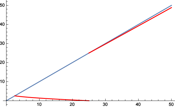
It should be helpful to preview the entire state space at the beginning. See Figure 3 for optimal strategy: continuation and stopping region in the two-dimensional diagram. The left panel is for presenting in a schematic drawing. For different values of , we see continuation regions and stopping region . The right panel is the real solution for this problem with parameters . According to the values of , we have four regions: (i) , (iii) , (ii) , and (iv) . We shall explain how to find the value function and optimal strategy for each region. Note that for the ease of exposition, we handle before we do .
(i) Let us start with . First we need to find . Plug this in (5.2) and examine the reward function in the transformed space:
Figure 4 -(i) shows the function on . For this , is concave in the neighborhood of and Case (a) in Section 4 applies. The map
Now we can find for . Following Section 5, we shall find the smallest concave majorant of that passes the origin and . For this particular , a diagram similar to Figure 2-(b) can be drawn: see Figure 4-(iii). The value function on the continuation region (red line in the graph) is
where .
In summary, the value function is

(i) Graph of when

(ii) The map to find

(iii) The value function (red) and (blue)
(ii) Let us move on to the region (before we examine ). See Figure 5-(i) for the graph of in the transformed space. In the neighborhood of , the reward is concave but We have for in this region, so that . On the other hand, for the reward function with this fixed , there is a point such that is the continuation region. Let us see this situation in the transformed space. See Figure 5-(i) again. At the point , the smallest concave majorant of is the line, from the origin, tangent to . Hence the value function is
where . Hence is the value function in region in Figure 3.
(iii) For , we have so that the point is in the stopping region. Moreover, there exist no points where the line from the origin becomes tangent to . Accordingly, the value function is
In our parameters, and is very close; .
(iv) Now we shall examine . As explained in Case (3) in Section 4, this satisfies . See (4.12). Following the argument there, . Accordingly, the value function is
| (5.3) |
This corresponds to region in Figure 3.
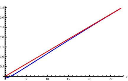
(i) Graph of and the tangent line when . .
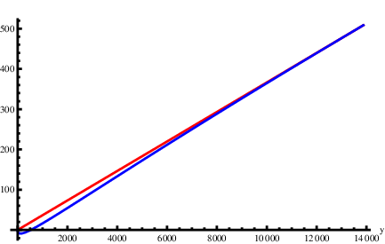
(ii) Graph of and the tangent line with
Appendix A Proof of Lemma 4.1
Lemma 4.1 is the following claim: Under the assumption of Proposition 4.1 with convex , we have
| (A.1) |
Proof.
(of the lemma) Recall (3.1) for the definition of . In view of (3.4), the probabilistic meaning of (4.2) is that is attained when one chooses the excursion level optimally in the following optimal stopping:
| (A.2) |
that is, if the excursion from does not reach the level of before reaches , one shall receive and otherwise, one shall receive the reward. By using the transformation (4.4), one needs to consider the function and the point in the -plane. Then the value function of (A.2) in this plane is the smallest concave majorant of which passes through the point . It follows that . As , it is clear that and . Suppose, for a contradiction, that we have
| (A.3) |
for all . This implies that the first term in (A.3) goes to from below and the third term goes to the same limit from above. While the second inequality always hold, the first inequality leads to a contradiction to the fact that the function is continuous for all .
Indeed, due to the monotonicity of in , we would have for all . Hence one cannot make the distance between and arbitrarily small without violating (A.3). This shows that there exists an such that implies that .
On the other hand, in (A.2), one could choose a stopping time that visits the left boundary , then by reading (3.4) with and , (A.2) becomes
for any . Since is a regular point, the last expectation can be arbitrarily close to unity, monotonically in (see page 89 [11]). Now suppose that there were no ’s such that . It follows that for any , we would have
Then by letting , it would be for all , which is absurd. Since the convergence of is monotone in , there exists an such that implies that . By using the second assumption in the statement of Proposition, in particular (4.7), for any , we have for . This completes the proof of Lemma 4.1. ∎
Appendix B On the smooth-fit principle
Reference is made to Section 4. Another representation of is still possible. Continue to fix . The smooth-fit principle is assumed to hold at an optimal point and we have as a continuation region with the line tangent to the function at . Then we have a first-order approximation of :
| (B.1) |
where
the slope of at . See (4.5). Equate equation (B.1) with (4.3) to obtain, for any sufficiently close to zero,
Since as ,
| (B.2) |
where the last equality is obtained by L’Hôpital’s rule. By multiplying on both sides and performing some algebra, we have
| (B.3) |
Let us mention some comments on the examples in Section 4. In Section 4.3.2 of the perpetual put, for the , as can be seen from the Figure 1, . Then (B.3) (see also (B.2)) reduces to a very simple form
which is the same as (4.13).
In the lookback option in Section 4.3.1, the case of was solved in the well-known [18]. For , the reward does not depend on , so that we have further simplification of . A straightforward computation from (B.3) below yields
| (B.4) |
where we write for simplicity. It can be confirmed that (B.4) for is the same as
in [18].
References
- [1] L. H. R. Alvarez. On the properties of r-excessive mappings for a class of diffusions. Ann. Appl. Probab., 13 (4):1517–1533, 2003.
- [2] L. H. R. Alvarez and P. Matomäki. Optimal stopping of the maximum process. J. Appl. Prob., 51:818–836, 2014.
- [3] F. Avram, A. E. Kyprianou, and M. R. Pistorius. Exit problems for spectrally negative Lévy processes and applications to (Canadized) Russion options. Ann. Appl. Probab., 14:215–235, 2004.
- [4] J. Bertoin. Lévy processes, volume 121 of Cambridge Tracts in Mathematics. Cambridge University Press, Cambridge, 1996.
- [5] A. N. Borodin and P. Salminen. Handbook of Brownian Motion - Facts and Formulae, Second Edition. Birkhäuser, Basel, Boston, Berlin, 2002.
- [6] E. Çinlar. Probability and Stochastics, volume 261 of Graduate Texts in Mathematics. Springer, Berlin Heidelberg, 2011.
- [7] S. Dayanik and I. Karatzas. On the optimal stopping problem for one-dimensional diffusions. Stochastic Process. Appl., 107 (2):173–212, 2003.
- [8] R. A. Doney. Some excursion calculations for spectrally one-sided Lévy processes. In Séminaire de Probabilités XXXVIII, volume 1857 of Lecture Notes in Math., pages 5–15. Springer, Berlin, 2005.
- [9] E. B. Dynkin. Markov Processes II. Springer, Berlin Heidelberg, 1965.
- [10] X. Guo and M. Zervos. options. Stoch. Proc. Appl., 120:1033–1059, 2007.
- [11] K. Itô and H. P. McKean Jr. Diffusion Processes and their Sample Paths. Springer, Berlin Heidelberg, 1974.
- [12] N. N. Lebedev. Special Functions and their Applications, revised edn. Dover Publications, New York, 1972.
- [13] C. Ott. Optimal stopping problems for the maximum process with upper and lower caps. Ann. Appl. Probab., 23:2327–2356, 2013.
- [14] G. Peskir. Optimal stopping of the maximum process: the maximality principle. Ann. Probab., 26:1614–1640, 1998.
- [15] H. Pham. Continuous-time Stochastic Control and Optimization with Financial Applications, volume 61 of Stochastic Modeling and Applied Probability. Springer, Berlin Heidelberg, 2009.
- [16] M. R. Pistorius. On exit and ergodicity of the spectrally one-sided Lévy process reflected at its infimum. J. Theoretical Probab., 17:183–220, 2004.
- [17] M. R. Pistorius. An excursion-theoretical approach to some boundary crossing problems and the Skorokhod embedding for reflected Lévy processes. In Séminaire de Probabilités XL, volume 1899 of Lecture Notes in Math., pages 278–307. Springer, Berlin, 2007.
- [18] L. Shepp and A. N. Shiryaev. The Russian otpion: reduced regret. Ann. Appl. Probab., 3:631–640, 1993.