On Sequential Elimination Algorithms for Best-Arm Identification in Multi-Armed Bandits

Multi-Armed Bandits (MAB) is a sequential decision-making framework addressing the exploration-exploitation dilemma [1, 2, 3, 4]. A player explores a finite set of arms sequentially, and pulling each of them results in a reward to the player. The problem has been studied for different rewards models. In the stochastic MAB, the rewards of each arm are assumed to be i.i.d. samples of an unknown, fixed distribution. Then, the player’s goal is to exploit the arm with largest expected reward as many times as possible to maximize the gain. In the literature, this objective has been translated to minimizing the cumulative regret, a comparison measure between the actual performance of the player versus a clairvoyant knowing the best arm in advance. Early studies on MAB dates back to a few decades ago, but the problem has surged a lot of renewed interest due to its modern applications. Though generally addressing sequential decision making problems, MAB has been studied in several engineering contexts such as web search and advertising, wireless cognitive radios, multi-channel communication systems, and Big-Data streaming (see e.g. [5, 6, 7, 8, 9, 10, 11] and references therein).

Departing from its classical setting (exploration-exploitation), many researchers have studied MAB in the pure-exploration framework. In this case, the player aims to minimize the simple regret which can be related to finding the best arm with a high probability [12]. As a result, the best-arm identification problem has received a considerable attention in the literature of machine learning[13, 14, 15, 16, 17, 12, 18, 19]. The problem has been viewed from two main standpoints: (i) the fixed-confidence setting, where the objective is to minimize the number of trials to find the best arm with a certain confidence, and (ii) the fixed-budget setting, where the player attempts to maximize the probability of correct identification given a fixed number of arm pulls. Best-arm identification has several applications including channel allocation as originally proposed in [12]. Consider the problem of channel allocation for mobile phone communication. Before the outset of communication, a cellphone (player) can explore the set of channels (arms) to find the best one to operate. Each channel feedback is noisy, and the number of trials (budget) is limited. The problem is hence an instance of best-arm identification, and minimizing the cumulative regret is not the right approach to the problem.

While both pure-exploration and exploration-exploitation setups are concerned with finding the best arm, they are quite different problems in nature. In fact, Bubeck et al. [17] establish that methods designed to minimize the cumulative regret (exploration-exploitation) can perform poorly for the simple-regret minimization (pure-exploration). More specifically, they proved that upper bounds on the cumulative regret yield lower bounds on the simple regret, i.e., the smaller the cumulative regret, the larger the simple regret. Therefore, one must adopt different strategies for optimal best-arm recommendation.

Notation: For integer $K$, we define $[K]:=\{1,\ldots,K\}$ to represent the set of positive integers smaller than or equal to $K$. We use $\left|S\right|$ to denote the cardinality of the set $S$. Throughout, the random variables are denoted in bold letters.

In this section, we propose our generic sequential elimination method and analyze its performance in the fixed budget setting. Consider a sequential elimination algorithm given budget $T$ of arm pulls. The algorithm maintains an active set initialized by the $K$ arms, and it proceeds for $R$ rounds to discard the arms sequentially until it is left by a single arm. Let us use $\left\lceil\cdot\right\rceil$ to denote the ceiling function. Then, for a constant $C$ and a decreasing, positive sequence $\{z_{r}\}_{r=1}^{R}$, set $n_{r}=\left\lceil(T-K)/(Cz_{r})\right\rceil$ at round $r\in[R]$, let the algorithm sample the remaining arms for $n_{r}-n_{r-1}$ times, and calculate the empirical average of rewards for each arm. If the algorithm dismisses $b_{r}$ arms with lowest average rewards, and we impose the constraint $\sum_{r=1}^{R}b_{r}=K-1$ on the sequence $\{b_{r}\}_{r=1}^{R}$, the algorithm outputs a single arm, the one that it hopes to be the best arm. This general point of view is summarized in Fig. 1 on the left side.

The choice of $C$ in the algorithm (see Fig. 1) must warrant that the budget constraint (3) holds. When we substitute $n_{r}$ into (3), we get

		$\displaystyle n_{R}+\sum_{r=1}^{R}b_{r}n_{r}=\left\lceil\frac{T-K}{Cz_{R}}\right\rceil+\sum_{r=1}^{R}b_{r}\left\lceil\frac{T-K}{Cz_{r}}\right\rceil$
		$\displaystyle~~~~~~~~~~~~~~~~\leq\frac{T-K}{Cz_{R}}+1+\sum_{r=1}^{R}b_{r}+\sum_{r=1}^{R}b_{r}\frac{T-K}{Cz_{r}}$
		$\displaystyle~~~~~~~~~~~~~~~~=K+\frac{T-K}{C}\left(\frac{1}{z_{R}}+\sum_{r=1}^{R}\frac{b_{r}}{z_{r}}\right)=T,$

where in the last line we used the condition $\sum_{r=1}^{R}b_{r}=K-1$. The following theorem provides an upper bound on the error probability of the algorithm.

It is already quite well-known that the sub-optimality $\Delta_{i}$ of each arm $i$ plays a key role in the identification quality; however, an important subsequent of Theorem 2 is that the performance of any sequential elimination algorithm also relies on the choice of $z_{r}$ which governs the constant $C$. In [12], Succ-Rej employs $z_{r}=K-r+1$, i.e., at each round the remaining arms are played equally often in total. This results in $C$ being of order $\log K$.

We now use the abstract form of the generic algorithm to specialize it to Nonlinear Sequential Elimination delineated in Fig. 1. The algorithm works with $b_{r}=1$ and $z_{r}={(K-r+1)}^{p}$ for a given $p>0$, and it is called “nonlinear” since $p$ is not necessarily equal to one. The choice of $p=1$ reduces the algorithm to Succ-Rej. In Section IV, we prove that in many regimes for arm gaps, $p\neq 1$ provides better theoretical results, and we further exhibit the efficiency in the numerical experiments in Section VI. The following proposition encapsulates the theoretical guarantee of the algorithm.

The performance of the algorithm does depend on the parameter $p$, but the choice is more qualitative rather than quantitative. For instance, if the sub-optimal arms are almost the same, i.e. $\Delta_{i}\approx\Delta$ for $i\in[K]$, noting the definition of $C_{p}$ and $H(p)$ in (5), we observe that $0<p<1$ performs better than $p>1$. In general, larger values for $p$ increase $H(p)$ and decrease $C(p)$. Therefore, there is a trade-off in choosing $p$. We elaborate on this issue in Sections IV and VI, where we observe that a wide range of values for $p$ can be used for tuning, and the trade-off can be addressed using either $0<p<1$ or $1<p\leq 2$.

We remark that in the proof of Theorem 2, the constant behind the exponent can be improved if one can avoid the union bounds. To do so, one needs to assume some structure in the sequence $\{g_{r}\}_{r=1}^{R}$. For instance, the authors in [18] leverage the fact that $g_{r+1}=\left\lceil g_{r}/2\right\rceil$ to avoid union bounds in Seq-Halv. The idea can be extended to when the ratio of $g_{r+1}/g_{r}$ is a constant independent of $r$.

Finally, while the result of Proposition 3 provides a general performance bound with respect to reward regimes, in the next section, we provide two important corollaries of the proposition to study several regimes for rewards, where we can simplify the bound and compare our result with other algorithms.

Inspired by numerical experiments carried out in the previous works [12, 18], we consider a few instances for sub-optimality of arms in this section, and we demonstrate how N-Seq-El fares in these cases. We would like to distinguish three general regimes that encompass interesting settings for sub-optimality and determine the values of $p$ for which we expect N-Seq-El to achieve faster identification rates:

• 1

  Arithmetic progression of gaps: In this case, $\Delta_{i}=(i-1)\Delta_{0}$ for $i>1$, where $\Delta_{0}$ is a constant.

• 2

  A large group of competitive, suboptimal arms: We recognize this case as when there exists a constant¹¹ 1 The choice of $\varepsilon$ must be constant with respect to $i$ and $K$. $\varepsilon\geq 0$ such that $\Delta_{i}/\Delta_{2}\leq 1+\varepsilon$ for arms $i\in S$, where $\left|S\right|$ grows linearly as a function of $K$, and for $i\notin S$, $\Delta_{i}/\Delta_{2}\geq i$.

• 3

  A small group of competitive, suboptimal arms: This case occurs when there exists a constant $\varepsilon\geq 0$ such that $\Delta_{i}/\Delta_{2}\leq 1+\varepsilon$ for $i\in S$, where $\left|S\right|$ is of constant order with respect to $K$, and for $i\notin S$, $\Delta_{i}/\Delta_{2}\geq i$.

We now state the following corollary of Proposition 3, which proves to be useful for our numerical evaluations. Note that the orders are expressed with respect to $K$.

We can now compare our algorithm with Succ-Rej and Seq-Halv  using the result of Corollary 4. Returning to Table I and calculating $H_{2}$ for Regimes $1$ to $3$, we can observe the following table,

which shows that with a right choice of $p$ for N-Seq-El, we can save a $\mathcal{O}(\log K)$ factor in the exponential rate comparing to other methods. Though we do not have a prior information on gaps to categorize them into one of the Regimes $1$ to $3$ (and then choose $p$), the choice of $p$ is more qualitative rather than quantitative. Roughly speaking: if the sub-optimal arms are almost the same $0<p<1$ performs better than $p>1$, and if there are a few real competitive arms, $p>1$ outperforms $0<p<1$. Therefore, the result of Corollary 4 is of practical interest, and we will show using numerical experiments (Section VI) that a wide range of values for $p$ can potentially result in efficient algorithms.

One should observe that the number of competitive arms is a key factor in tuning $p$. We now provide another corollary of Proposition 3, which presents the suitable range of parameter $p$ given the growth rate of competitive arms as follows.

The corollary above indicates that a side information in the form of the number of competitive arms (in the order) can help us tune the input parameter $p$. The corollary exhibits a smooth interpolation between when the competitive arms are small versus when they are large. Perhaps, the most interesting regime is the middle row, where the choice of $p$ is given as a function of the number of arms $K$. Consider the following example where we calculate the choice of $p$ for $f_{K}=K^{\gamma}$, where $\gamma\in\{0.3,0.5,0.7\}$.

As we can see in the table above, since the condition on $p$ depends in logarithmic orders on $K$ and $f_{K}$, we have flexibility to tune $p$ even for very large $K$. However, we only use $K\in\{40,120\}$ for the numerical experiments in Section VI, since the time-complexity of Monte Carlo simulations is prohibitive on large number of arms.

In the previous sections, we considered a scenario in which pulling an arm yields only the reward of the chosen arm. However, there exist applications where pulling an arm can additionally result in some side observations. For a motivative example, consider the problem of web advertising, where an ad placer offers an ad to a user and receives a reward only if the user clicks on the ad. In this example, if the user clicks on a vacation ad, the ad placer receives the side information that the user could have also clicked on ads for rental cars. The value of side observations in the stochastic MAB was studied in [22] for exploration-exploitation setting. The side-observation model is described via an undirected graph that captures the relationship between the arms. Once an arm is pulled, the player observes the reward of the arm as well as its neighboring arms. In exploration-exploitation settings, the analysis of MAB with side observations relies on the cliques of the graph [21, 22]. In this section, we would like to consider the impact in the pure-exploration setting.

In the pure-exploration, we minimize the simple regret rather than the cumulative regret, and therefore, the player’s best bets are the most connected arms resulting in more observations. Now consider a partition of the set $[K]$ into $M$ blocks $\{V_{i}\}_{i=1}^{M}$ such that each $V_{i}$ contains a star graph, i.e., there exists an arm in $V_{i}$ connected to all other arms. Given such partition, the player can follow a simple rule to leverage side observations and eliminate blocks one by one. The idea is to sample the central arm in each block, which reveals the rewards for all the arms in that block. At round $r$, sample the remaining blocks (the central arms of each block) for $n_{r}-n_{r-1}$ times, and find the arm with largest average reward in each block. With the best arms of all blocks at hand, remove the block whose best arm is the worst comparing to other blocks. Continue the sampling until only one block is left, and output the arm with largest average reward in the final block as the best arm. The algorithm, called Sequential Block Elimination, is summarized in Fig. 2, and its performance is characterized in the following theorem.

The theorem indicates that once we can partition the arms into $M$ blocks, the complexity measure $H(p)$ need not be maximized over $K$ arms. Instead, it is maximized over the top $M$ arms. The improvement must be more visible in the settings that arms are roughly as competitive as each other, since we can slow down the linear growth of $K$ by $M$.

As a final note, $M=K$ recovers the fully bandit (no side observation) setting with $V=1$, and we observe that in such case, we recover the result of Proposition 3 from Theorem 6 in the rate of exponential decay. However, the constant behind the exponential would change from $K-1$ in Proposition 3 to $K$ in Theorem 6. This is the artifact of an extra term contributing to the upper bound, which can be removed for the case $M=K$.

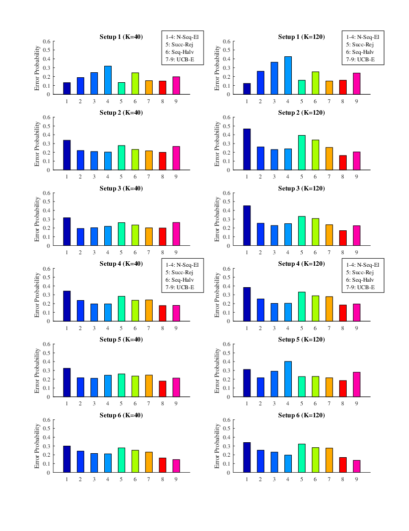
In this section, we empirically evaluate our algorithm on the settings perviously studied in [12, 18]. In these experiments, we compare N-Seq-El with Succ-Rej, Seq-Halv, and UCB-E. Though we include UCB-E proposed in [12] as a benchmark, we remark that the algorithm requires a prior knowledge of a parameter that depends on $H_{1}$ defined in (4). The adaptive version of UCB-E was also developed in [12]. The algorithm (called AUCB-E) does not need prior knowledge of $H_{1}$, and it calculates the parameter online. The experiments in [18] suggest that for $T\approx H_{1}$, Succ-Rej, Seq-Halv, and UCB-E outperform AUCB-E, and it is not surprising that the prior knowledge of $H_{1}$ must give UCB-E an advantage over AUCB-E.

We consider Bernoulli distribution on the rewards, assuming that the expected value of Bernoulli distribution for the best arm is $\mu_{1}=0.7$. In what follows, we use the notation $x\colon\hskip-2.84544pty$ to denote integers in $[x,y]$. We examine the following setups for two values of arm numbers $K\in\{40,120\}$:

• 1

  One group of suboptimal arms: $\mu_{2\colon\hskip-2.84544ptK}=0.6$.

• 2

  Two groups of suboptimal arms: $\mu_{2:m}=0.7-\frac{2}{K}$, $\mu_{m+1:K}=0.4$, and $m=\left\lceil\log\frac{K}{2}+1\right\rceil$.

• 3

  Three groups of suboptimal arms: $\mu_{2:m}=0.7-\frac{2}{K}$, $\mu_{m+1:2m}=0.7-\frac{4}{K}$, $\mu_{2m+1:K}=0.4$, and $m=\left\lceil\log\frac{K}{2}+1\right\rceil$.

• 4

  Arithmetic progression: $\Delta_{i}=\frac{0.6(i-1)}{K-1}$ for $i=2\colon\hskip-2.84544ptK$.

• 5

  Geometric progression: $\Delta_{i}=0.01(1+\frac{4}{K})^{i-2}$ for $i=2\colon\hskip-2.84544ptK$.

• 6

  One real competitive arm: $\mu_{2}=0.7-\frac{1}{2K}$ and $\mu_{3:K}=0.2$.

We run $4000$ experiments for each setup with specific $K$, and the misidentification probability is averaged out over the experiment runs. The budget $T$ considered in each setup is equal to $\left\lceil H_{1}\right\rceil$ in the corresponding setup following [12, 18]. Fig. 3 illustrates the performance of each algorithm in different setups. The height of each bar depicts the misidentification probability, and the index guideline is as follows: (i) indices 1-4: N-Seq-El with parameter $p=0.75,1.35,1.7,2$. (ii) index 5: Succ-Rej. (iii) index 6: Seq-Halv. (iv) indices 7-9: UCB-E with parameter $a=cT/H_{1}$, for $c=1,2,4$. The legends are the same for all the plots, and we remove some of them to avoid clutter.

The results are consistent with Corollary 4, and the following comments are in order:

• •

  Setup 1 perfectly relates to Regime 2 in Corollary 4 ($\varepsilon=0$). While any choice of $0<p<1$ gives an $\mathcal{O}(K)$ rate, the rate deteriorates to $\mathcal{O}(K^{p})$ by choosing $1<p\leq 2$. Therefore, only the the choice of $p=0.75$ is appropriate for N-Seq-El. This choice joined with Succ-Rej (which amounts to our algorithm with $p=1$) outperform others even UCB-E.

• •

  Setup 4 defines Regime 1 in Corollary 4. Accordingly, choice of $1<p\leq 2$ outperforms Succ-Rej and Seq-Halv, and $p=1.7,2$ prove to be competitive to UCB-E.

• •

  In Setups 2-3, the number of competitive arms grows with $\mathcal{O}(\log K)$, but they can be considered close to Regime 3 in Corollary 4 as the growth is sub-linear. Also, Setup 6 is the ideal match for Regime 3 in Corollary 4. Therefore, any choice of $1<p\leq 2$ should be suitable in these cases. We observe that for $p=1.35,1.7,2$, N-Seq-El outperforms Succ-Rej and Seq-Halv, while being quite competitive to UCB-E in Setups 2-3 for $K=40$.

• •

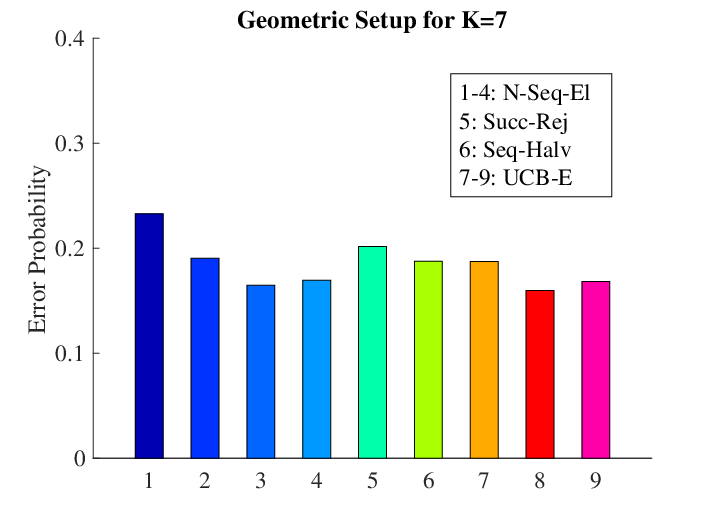
  In Setup 5, we were expecting to observe good performance for $1<p\leq 2$. While we do see that for $K=40$, N-Seq-El outperforms Succ-Rej and Seq-Halv with $p=1.35,1.7$, the performance is not quite satisfactory for $K=120$ (only $p=1.35$ performs well). A potential reason is that we want to keep the rewards bounded in $[0,1]$, thereby choosing the geometric rate for $\Delta_{i}$ so slow that it is dominated by ${i}^{p}$ rate in (5). To support our argument, we present a complementary evaluation of this case for a small $K$, where we can use faster geometric growth.

• •

  As a final remark, note that in consistent with Table II, for relevant cases we observe an improvement of performance when $K$ increases. For instance, in Setup 1 with $p=0.75$, the ratio of misidentification probability of N-Seq-El to Seq-Halv increases from $1.84~(K=40)$ to $2.06~(K=120)$, or in Setup 4 with $p=2$, the ratio of misidentification probability of N-Seq-El to Succ-Rej increases from $1.43~(K=40)$ to $1.63~(K=120)$.

We considered best-arm identification in the stochastic multi-armed bandits, where a player is given a certain budget to explore a finite number of arms. The player’s objective is to detect the arm with largest expected reward. We contribute to the literature of best-arm identification by (i) unifying sequential elimination algorithms under a general framework, which introduces a novel performance metric for this class of algorithms, (ii) developing a nonlinear sequential elimination algorithm with provable theoretical and practical guarantees, (iii) and establishing a theoretical result on the value of side observations in the pure-exploration setting.

Having established that we gain advantage from nonlinear budget allocation, an important future direction is to propose a method that starts with a specific nonlinear rate and fine-tunes the rate according to the problem environment. The main challenge is that the quantity $C$ should perhaps be time-varying, and its value needs to be cautiously controlled by the algorithm, so that the algorithm does not overspend the budget.

We gratefully acknowledge the support of DARPA under grant numbers N66001-15-C-4028 and W911NF-14-1-0508. We thank Prof. Masahiro Yukawa (Keio University) for his helpful comments. We also thank Dr. Ahmad Beirami and Dr. Hamed Farhadi for many helpful discussions.

Recall that $\mathbf{G}_{r}$ denotes the set of arms not eliminated by the start of round $r$ with $g_{r}=\left|\mathbf{G}_{r}\right|$ being its cardinality. Also, $\mathbf{B}_{r}$ represents the set of arms that we decide to discard after playing round $r$ with $b_{r}=\left|\mathbf{B}_{r}\right|$ denoting its cardinality. It evidently holds that $\mathbf{G}_{r+1}=\mathbf{G}_{r}\setminus\mathbf{B}_{r}$ for $r\in[R]$. Therefore,

$\displaystyle\mathbb{P}\left(\mathbf{G}_{R+1}\neq\{1\}\right)=\mathbb{P}\left(1\in\cup_{r=1}^{R}\mathbf{B}_{r}\right)=\sum_{r=1}^{R}\mathbb{P}\left(1\in\mathbf{B}_{r}\right),$

(6)

since the sets of removed arms at each round are disjoint, i.e. $\mathbf{B}_{i}\cap\mathbf{B}_{j}=\emptyset$ for $i\neq j$. We can then write

$\displaystyle\mathbb{P}\left(1\in\mathbf{B}_{r}\right)=\sum_{G_{r}}\mathbb{P}\left(1\in\mathbf{B}_{r}~|~\mathbf{G}_{r}=G_{r}\right)\mathbb{P}\left(\mathbf{G}_{r}=G_{r}\right).$

(7)

Now for any particular $G_{r}$, consider the worst $b_{r}$ arms, i.e., the bottom $b_{r}$ arms when arms are ordered in terms of (true) expected value. If the best arm (arm $1$) is set to be eliminated at the end of round $r$, its empirical average must be less than at least one of these $b_{r}$ arms. In the case that $G_{r}=\{1,2,\ldots,g_{r}\}$, the bottom $b_{r}$ arms would be $\{g_{r}-b_{r}+1,\ldots,g_{r}\}$. Therefore, recalling that $\bar{\mathbf{x}}_{i,n}$ denotes the average reward of pulling arm $i$ for $n$ times, and using Hoeffding’s inequality (Fact 1), we get

		$\displaystyle\mathbb{P}\left(1\in\mathbf{B}_{r}~|~\mathbf{G}_{r}=\{1,2,\ldots,g_{r}\}\right)$
		$\displaystyle~~~~~~~~~~~~~\leq\sum_{i=g_{r}-b_{r}+1}^{g_{r}}\mathbb{P}\left(\bar{\mathbf{x}}_{1,n_{r}}\leq\bar{\mathbf{x}}_{i,n_{r}}\right)$
		$\displaystyle~~~~~~~~~~~~~\leq\vphantom{\sum_{i=g_{r}-b_{r}+1}^{g_{r}}\mathbb{P}\left(\bar{\mathbf{x}}_{1,n_{r}}\leq\bar{\mathbf{x}}_{i,n_{r}}\right)}b_{r}\exp\left(-2n_{r}\Delta_{g_{r}-b_{r}+1}^{2}\right)$
		$\displaystyle~~~~~~~~~~~~~=b_{r}\exp\left(-2n_{r}\Delta_{g_{r+1}+1}^{2}\right),$		(8)

where the last step is due to the fact that $g_{r+1}=g_{r}-b_{r}$. In any other case for $G_{r}$ the best of the worst $b_{r}$ arms cannot be better than arm $g_{r}-b_{r}+1$. As a result, combining (7) and (8), we obtain

	$\displaystyle\mathbb{P}\left(1\in\mathbf{B}_{r}\right)$	$\displaystyle\leq\sum_{G_{r}}b_{r}\exp\left(-2n_{r}\Delta_{g_{r+1}+1}^{2}\right)\mathbb{P}\left(\mathbf{G}_{r}=G_{r}\right)$
		$\displaystyle=b_{r}\exp\left(-2n_{r}\Delta_{g_{r+1}+1}^{2}\right).$

Then, in view of (6) we derive

		$\displaystyle\mathbb{P}\left(\mathbf{G}_{R+1}\neq\{1\}\right)\leq\sum_{r=1}^{R}b_{r}\exp\left(-2n_{r}\Delta_{g_{r+1}+1}^{2}\right)$
		$\displaystyle~~~~~~~~~~\leq R\max_{r\in[R]}\{b_{r}\}\max_{r\in[R]}\left\{\exp\left(-2n_{r}\Delta_{g_{r+1}+1}^{2}\right)\right\}.$

Noting the fact that $n_{r}=\left\lceil\frac{T-K}{Cz_{r}}\right\rceil\geq\frac{T-K}{Cz_{r}}$, we can use above to conclude that

		$\displaystyle\mathbb{P}\left(\mathbf{G}_{R+1}\neq\{1\}\right)\leq$
		$\displaystyle~~~~~~~~~~~~~R\max_{r\in[R]}\{b_{r}\}\max_{r\in[R]}\left\{\exp\left(-\frac{T-K}{Cz_{r}}2\Delta_{g_{r+1}+1}^{2}\right)\right\},$

which completes the proof. ∎

We point out that the algorithm is a special case of General Sequential Elimination where $R=K-1$, $b_{r}=1$, $g_{r}=K-r+1$, and $z_{r}={(K-r+1)}^{p}$. The proof then follows immediately from the result of Theorem 2. ∎

The proof follows by substituting each case in (5). We need to understand the order of $C_{p}$ and $H(p)$ for different regimes of $p$. Let us start by

$$C_{p}=2^{-p}+\sum_{r=2}^{K}r^{-p},$$

and noting that for any $p>1$, $C_{p}$ is a convergent sum when $K\rightarrow\infty$. Therefore, for the regime $p>1$, the sum is a constant, i.e., $C_{p}=\mathcal{O}(1)$. On the other hand, consider $q\in(0,1)$, and note that the sum is divergent, and for large $K$ we have $C_{q}=\mathcal{O}(K^{1-q})$. Now, let us analyze

$$H(p)=\max_{i\neq 1}\frac{i^{p}}{\Delta_{i}^{2}}.$$

For Regime 1, since $\Delta_{i}=(i-1)\Delta_{0}$, for $p\in(1,2)$, we have

	$\displaystyle H(p)$	$\displaystyle=\max_{i\neq 1}\left(1+\frac{1}{i-1}\right)^{p}\frac{(i-1)^{p-2}}{\Delta_{0}^{2}}$
		$\displaystyle\leq\max_{i\neq 1}\left(1+\frac{1}{i-1}\right)^{p}\frac{1}{\Delta_{0}^{2}}=\frac{1.5^{p}}{\Delta_{0}^{2}},$

which is of constant order with respect to $K$. Therefore, the product $C_{p}H(p)=\mathcal{O}(1)$.

For Regime 2, we have

$$H(q)=\max_{i\neq 1}\frac{i^{q}}{\Delta_{i}^{2}}\leq\max_{i\neq 1}\frac{i^{q}}{\Delta_{2}^{2}}\leq\frac{K^{q}}{\Delta_{2}^{2}},$$

and the maximum order can be achieved as the number of arms close to the second best arm grows linearly in $K$. Combining with $C_{q}=\mathcal{O}(K^{1-q})$, the product $C_{q}H(q)=\mathcal{O}(K)$.

For Regime 3, if $i\in S$, we have

$$\max_{i\in S}\frac{i^{p}}{\Delta_{i}^{2}}=\mathcal{O}(1),$$

since the cardinality of $S$ is of constant order with respect to $K$. On the other hand, since $1<p\leq 2$, we have

$$\max_{i\notin S}\frac{i^{p}}{\Delta_{i}^{2}}\leq\max_{i\notin S}\frac{i^{p}}{i^{2}\Delta_{2}^{2}}=\max_{i\notin S}\frac{i^{p-2}}{\Delta_{2}^{2}}=\mathcal{O}(1).$$

Therefore, $H(p)$ is of constant order, and combining with $C_{p}=\mathcal{O}(1)$, the product $C_{p}H(p)=\mathcal{O}(1)$. ∎

According to calculations in the previous proof, we have that $C_{p}=\mathcal{O}(K^{1-p})$ for $0<p<1$, and $C_{p}=\mathcal{O}(1)$ for $1<p\leq 2$. In order to find out the order of $H(p)$ and $H(2)$, we should note that

$$\mathcal{O}(H(p))=\mathcal{O}\left(\max_{i\in S}\frac{i^{p}}{\Delta_{i}^{2}}\right)=\mathcal{O}\left(\max_{i\in S}\frac{i^{p}}{\Delta_{2}^{2}}\right)=f_{K}^{p},$$

and we simply have $\mathcal{O}(H_{2})=\mathcal{O}(H(1))=f_{K}$. Now returning to Table I, we must compare $\mathcal{O}(H(p)C_{p})=f_{K}^{p}\mathcal{O}(C_{p})$ and $\mathcal{O}(H_{2}\log K)=f_{K}\log K$ for all three the rows given in Table III.

Row 1: In the case that $1\leq f_{K}\leq\log K$, for any choice of $1<p\leq 2$, since $C_{p}=\mathcal{O}(1)$, we always have

$$f_{K}^{p}\leq f_{K}\log K\Leftrightarrow f_{K}^{p-1}\leq\log K.$$

Row 3: In the case that $\frac{K}{\log K}\leq f_{K}\leq K-1$, for any choice of $0<p<1$, since $C_{p}=\mathcal{O}(K^{1-p})$, we have

$\displaystyle f_{K}^{p}\mathcal{O}(C_{p})=f_{K}^{p}K^{1-p}=f_{K}\left(\frac{K}{f_{K}}\right)^{1-p}\leq f_{K}\log K.$

Row 2: In this case, we have that $\log K<f_{K}<\frac{K}{\log K}$. To prove the claim in the Table III, we have to break down the analysis into two cases:

References

- [1] T. L. Lai and H. Robbins, “Asymptotically efficient adaptive allocation rules,” Advances in applied mathematics, vol. 6, no. 1, pp. 4–22, 1985.
- [2] P. Auer, N. Cesa-Bianchi, and P. Fischer, “Finite-time analysis of the multiarmed bandit problem,” Machine learning, vol. 47, no. 2-3, pp. 235–256, 2002.
- [3] P. Auer, N. Cesa-Bianchi, Y. Freund, and R. E. Schapire, “The nonstochastic multiarmed bandit problem,” SIAM Journal on Computing, vol. 32, no. 1, pp. 48–77, 2002.
- [4] S. Bubeck and N. Cesa-Bianchi, “Regret analysis of stochastic and nonstochastic multi-armed bandit problems,” Machine Learning, vol. 5, no. 1, pp. 1–122, 2012.
- [5] A. Mahajan and D. Teneketzis, “Multi-armed bandit problems,” in Foundations and Applications of Sensor Management. Springer, 2008, pp. 121–151.
- [6] K. Liu and Q. Zhao, “Distributed learning in multi-armed bandit with multiple players,” IEEE Transactions on Signal Processing, vol. 58, no. 11, pp. 5667–5681, 2010.
- [7] K. Wang and L. Chen, “On optimality of myopic policy for restless multi-armed bandit problem: An axiomatic approach,” IEEE Transactions on Signal Processing, vol. 60, no. 1, pp. 300–309, 2012.
- [8] S. Vakili, K. Liu, and Q. Zhao, “Deterministic sequencing of exploration and exploitation for multi-armed bandit problems,” IEEE Journal of Selected Topics in Signal Processing, vol. 7, no. 5, pp. 759–767, 2013.
- [9] D. Kalathil, N. Nayyar, and R. Jain, “Decentralized learning for multiplayer multiarmed bandits,” IEEE Transactions on Information Theory, vol. 60, no. 4, pp. 2331–2345, 2014.
- [10] S. Bagheri and A. Scaglione, “The restless multi-armed bandit formulation of the cognitive compressive sensing problem,” IEEE Transactions on Signal Processing, vol. 63, no. 5, pp. 1183–1198, 2015.
- [11] K. Kanoun, C. Tekin, D. Atienza, and M. Van Der Schaar, “Big-data streaming applications scheduling based on staged multi-armed bandits,” IEEE Transactions on Computers, 2016.
- [12] J.-Y. Audibert and S. Bubeck, “Best arm identification in multi-armed bandits,” in COLT-23th Conference on Learning Theory-2010, 2010, pp. 13–p.
- [13] E. Even-Dar, S. Mannor, and Y. Mansour, “PAC bounds for multi-armed bandit and markov decision processes,” in Computational Learning Theory. Springer, 2002, pp. 255–270.
- [14] S. Mannor and J. N. Tsitsiklis, “The sample complexity of exploration in the multi-armed bandit problem,” The Journal of Machine Learning Research, vol. 5, pp. 623–648, 2004.
- [15] E. Even-Dar, S. Mannor, and Y. Mansour, “Action elimination and stopping conditions for the multi-armed bandit and reinforcement learning problems,” The Journal of Machine Learning Research, vol. 7, pp. 1079–1105, 2006.
- [16] S. Bubeck, R. Munos, and G. Stoltz, “Pure exploration in multi-armed bandits problems,” in Algorithmic Learning Theory. Springer, 2009, pp. 23–37.
- [17] ——, “Pure exploration in finitely-armed and continuous-armed bandits,” Theoretical Computer Science, vol. 412, no. 19, pp. 1832–1852, 2011.
- [18] Z. Karnin, T. Koren, and O. Somekh, “Almost optimal exploration in multi-armed bandits,” in Proceedings of the 30th International Conference on Machine Learning (ICML-13), 2013, pp. 1238–1246.
- [19] V. Gabillon, M. Ghavamzadeh, and A. Lazaric, “Best arm identification: A unified approach to fixed budget and fixed confidence,” in Advances in Neural Information Processing Systems, 2012, pp. 3212–3220.
- [20] A. Carpentier and A. Locatelli, “Tight (lower) bounds for the fixed budget best arm identification bandit problem,” in 29th Annual Conference on Learning Theory, 2016, pp. 590–604.
- [21] S. Mannor and O. Shamir, “From bandits to experts: On the value of side-observations,” in Advances in Neural Information Processing Systems, 2011, pp. 684–692.
- [22] S. Caron, B. Kveton, M. Lelarge, and S. Bhagat, “Leveraging side observations in stochastic bandits,” Uncertainty in Artificial Intelligence (UAI), 2012.
- [23] S. Buccapatnam, A. Eryilmaz, and N. B. Shroff, “Stochastic bandits with side observations on networks,” in The 2014 ACM international conference on Measurement and modeling of computer systems, 2014, pp. 289–300.
- [24] K. Jamieson, M. Malloy, R. Nowak, and S. Bubeck, “lil’ucb: An optimal exploration algorithm for multi-armed bandits,” in Proceedings of The 27th Conference on Learning Theory, 2014, pp. 423–439.
- [25] K. Jamieson and R. Nowak, “Best-arm identification algorithms for multi-armed bandits in the fixed confidence setting,” in Information Sciences and Systems (CISS), 2014 48th Annual Conference on. IEEE, 2014, pp. 1–6.
- [26] E. Kaufmann and S. Kalyanakrishnan, “Information complexity in bandit subset selection,” in Conference on Learning Theory, 2013, pp. 228–251.
- [27] E. Kaufmann, O. Cappé, and A. Garivier, “On the complexity of best-arm identification in multi-armed bandit models,” Journal of Machine Learning Research, vol. 17, no. 1, pp. 1–42, 2016.
- [28] D. Russo, “Simple bayesian algorithms for best arm identification,” in 29th Annual Conference on Learning Theory, 2016.
- [29] S. Kalyanakrishnan and P. Stone, “Efficient selection of multiple bandit arms: Theory and practice,” in Proceedings of the 27th International Conference on Machine Learning (ICML-10), 2010, pp. 511–518.
- [30] S. Kalyanakrishnan, A. Tewari, P. Auer, and P. Stone, “PAC subset selection in stochastic multi-armed bandits,” in Proceedings of the 29th International Conference on Machine Learning (ICML-12), 2012, pp. 655–662.
- [31] S. Bubeck, T. Wang, and N. Viswanathan, “Multiple identifications in multi-armed bandits,” in Proceedings of The 30th International Conference on Machine Learning, 2013, pp. 258–265.
- [32] Y. Zhou, X. Chen, and J. Li, “Optimal PAC multiple arm identification with applications to crowdsourcing,” in Proceedings of the 31st International Conference on Machine Learning (ICML-14), 2014, pp. 217–225.
- [33] T. Pepels, T. Cazenave, M. H. Winands, and M. Lanctot, “Minimizing simple and cumulative regret in monte-carlo tree search,” in Computer Games. Springer, 2014, pp. 1–15.
- [34] Y.-C. Liu and Y. Tsuruoka, “Regulation of exploration for simple regret minimization in monte-carlo tree search,” in IEEE Conference on Computational Intelligence and Games (CIG), 2015, pp. 35–42.