A Computationally Efficient Projection-Based Approach for Spatial Generalized Linear Mixed Models
Abstract
Inference for spatial generalized linear mixed models (SGLMMs) for high-dimensional non-Gaussian spatial data is computationally intensive. The computational challenge is due to the high-dimensional random effects and because Markov chain Monte Carlo (MCMC) algorithms for these models tend to be slow mixing. Moreover, spatial confounding inflates the variance of fixed effect (regression coefficient) estimates. Our approach addresses both the computational and confounding issues by replacing the high-dimensional spatial random effects with a reduced-dimensional representation based on random projections. Standard MCMC algorithms mix well and the reduced-dimensional setting speeds up computations per iteration. We show, via simulated examples, that Bayesian inference for this reduced-dimensional approach works well both in terms of inference as well as prediction; our methods also compare favorably to existing “reduced-rank” approaches. We also apply our methods to two real world data examples, one on bird count data and the other classifying rock types.
Keywords: random projection, non-Gaussian spatial data, spatial confounding, Gaussian process, MCMC mixing
1 Introduction
Gaussian and non-Gaussian spatial data arise in a number of disciplines, for example, species counts in ecology, tree presence-absence data, and disease incidence data. Models for such data are important for scientific applications, for instance when fitting spatial regression models or when interpolating observations across continuous spatial domains. Spatial generalized linear mixed models (SGLMMs) are popular and flexible models for spatial data, both for continuous spatial domain or “point-referenced” data (Diggle et al.,, 1998), where the spatial dependence is captured by random effects modeled using a Gaussian process, as well as for lattice or areal data (Besag et al.,, 1991, Rue and Held,, 2005, cf.) where dependence is captured via random effects modeled with Gaussian Markov random fields. SGLMMs have become very popular in a wide range of disciplines. In practice, however, SGLMMs pose some computational and inferential challenges: (i) computational issues due to high-dimensional random effects that are typically strongly cross-correlated – these often result in slow mixing Markov chain Monte Carlo (MCMC) algorithms; (ii) computations involving large matrices; and (iii) spatial confounding between fixed and random effects, which can lead to variance-inflated estimation of regression coefficients (Reich et al.,, 2006, Hughes and Haran,, 2013, Hanks et al.,, 2015). In this manuscript we provide an approach for reducing the dimensions of the spatial random effects in SGLMM models. Our approach simultaneously addresses both computational issues as well as the confounding issue.
There is a large literature on fast computational methods for spatial models (cf. Cressie and Johannesson,, 2008, Banerjee et al.,, 2008, Higdon,, 1998, Shaby and Ruppert,, 2012, Datta et al.,, 2016, among many others). These methods have been very useful in practice, but they largely focus on linear (Gaussian) spatial models and do not consider the spatial confounding issue. The predictive process approach (Banerjee et al.,, 2008) has been an important contribution to the literature, and has also been studied in the SGLMM context. However, the predictive process approach requires that users provide reference knots, which can be challenging to specify; our method is more automated. We also find that in some cases we obtain similar performance to the predictive process at far lower computational cost. Crucially, our approach is also able to easily address the spatial confounding issue. INLA (Rue et al.,, 2009) provides a sophisticated numerical approximation approach for SGLMMs. As we later discuss, INLA may be used in combination with the projection-based reparameterization approach we develop in this manuscript. This is useful for addressing confounding while also reducing computational costs.
Restricted spatial regression models for areal and point-referenced spatial data (Reich et al.,, 2006, Hanks et al.,, 2015) address the confounding issue. However, these models are computationally intensive for large data sets. For areal data, Hughes and Haran, (2013) alleviate confounding in a computationally efficient manner by proposing a reparameterization that utilizes the underlying graph to reduce the dimension of random effects. To our knowledge, no existing approach alleviates spatial confounding and is computationally efficient for point-referenced non-Gaussian data. In this manuscript we describe a novel method that utilizes the principal components of covariance matrices to achieve fast computation for fitting traditional SGLMMs as well as restricted spatial regression.
Our method relies on the random projections algorithm (Banerjee et al.,, 2012, Sarlos,, 2006, Halko et al.,, 2011), which allows a fast approximation of the leading eigencomponents. We show how we can build upon this projection-based approach to address the computational and inferential challenges of SGLMMs. The outline of the remainder of the paper is as follows. In Section 2, we introduce spatial linear mixed models and explain how a generalized linear model formulation of these models is appropriate for non-Gaussian observations. We also examine the computational challenges and some current approaches. In Section 3, we explain spatial confounding, how it affects interpretation of regression parameters, and describe how to alleviate confounding via orthogonalization. In Section 4, we describe our projection-based approach for both the continuous domain and lattice case. We study the inference and prediction performance of the proposed method via a simulation study in Section 5, and study our method in the context of applications in Section 6. We conclude with a discussion of our work in Section 7.
2 Spatial Models
2.1 Spatial linear models
Let denote an observation, and a dimensional vector of covariates at location in a spatial domain , where is typically 2 or 3. Given data locations , the observations may show residual spatial structure after controlling for . This can be taken into account by including spatially dependent random effects to model the residual dependence,
| (1) |
where are regression parameters. is a small-scale (nugget) spatial effect/measurement error process, modeled as an uncorrelated Gaussian process with mean 0 and variance . For point-referenced data, the random effects are typically modeled by a zero-mean stationary Gaussian process with a positive definite covariance function . Hence, for a finite set of locations, follows a multivariate normal distribution , with .
A commonly used class of covariance functions, assuming stationarity and isotropy, is the Matérn class (Stein,, 1999),
where denotes the Euclidean distance between pairs of locations, is a variance parameter, and is a positive definite correlation function parameterized by , the spatial range parameter, and , the smoothness parameter. is the gamma function, and is the modified Bessel function of the second kind.
2.2 Spatial generalized linear mixed models
A popular way to model spatial non-Gaussian data is by using spatial generalized linear mixed models (SGLMMs) (Diggle et al.,, 1998, Haran,, 2011, cf.). Let denote a non-Gaussian spatial field, and a known link function. Then, the conditional mean, may be modeled as
| (2) |
Conditional on , are mutually independent, following a classical generalized linear model (Diggle et al.,, 1998, cf.). We provide two commonly used examples of SGLMMs for spatial binary and count data to illustrate our projection-based approach, the Poisson with log link and binary with logit link respectively. The projection-based approach presented in this paper generalizes to other link functions and observation models, as well as to cases where an additional nugget term is added to the model (2) (Berrett and Calder,, 2016, cf.). Details for the nugget model are provided in the supplement S.5.
2.3 Model fitting and computational challenges
The hierarchical structure of spatial models makes it convenient to use a Bayesian inferential approach. Often in practice, we fix the value of and assign prior, , to parameters and where , then use Markov Chain Monte Carlo (MCMC) to sample from the posterior . Fitting SGLMMs generally requires the evaluation of an n-dimension multivariate normal likelihood for every MCMC iteration, with matrix operations of order floating point operations (flops). There are often strong correlations between the fixed and random effects (Hodges and Reich,, 2010), and strong cross-correlations among the spatially dependent random effects. It is well known that this dependence is often an important cause of poor mixing in standard MCMC algorithms (Christensen et al.,, 2006, Haran et al.,, 2003, Rue and Held,, 2005, cf.). Furthermore, when the data locations are near each other, the covariance matrix may be near singular, resulting in numerical instabilities (Banerjee et al.,, 2012). These issues motivate the development of our reduced-dimensional approach to inference for SGLMMs.
Considerable work has been done to address the above issues in the linear case, where model inference and prediction are based on the marginal distribution . Several methods rely on low rank approximations or multi-resolution approaches to reduce computations involving the covariance matrix (Banerjee et al.,, 2012, Sang and Huang,, 2012, Nychka et al.,, 2015, Cressie and Johannesson,, 2008, cf.). However, these methods do not readily extend to SGLMMs because they assume that the random effects may be “marginalized out” in closed form. For SGLMMs, this is generally not possible. Sengupta and Cressie, (2013), Sengupta et al., (2016) extended low rank approximation method to SGLMM setting. They used bi-square basis functions to represent random effects with addition random noise to capture fine-scale-variation. Their model for the spatial random effects has the form , where denotes the basis functions, is a vector of random effects with unknown , and independent Gaussian noise . Due to the high dimension of the random effects, the authors proposed empirical-Bayesian inference, which combines Laplace approximations in an expectation-maximization (EM) algorithm to obtain parameter estimates. A notable exception is the predictive process approach (Banerjee et al.,, 2008), where the extension to SGLMMs has been well studied. This approach replaces random effect by , the realization of at reference knots ; , where denotes the covariance matrix . Correspondingly, is approximated by a low rank matrix , where denotes the covariance matrix . This method can be applied to both the linear and the generalized case. However, Finley et al., (2009) points out that the predictive process underestimates the variance of and proposed a modified predictive process by defining , where . For the linear case, this adjustment adds little extra computation. However, for the SGLMM case, the modified predictive process puts us back to working with a high-dimensional random effect . Furthermore, determining the number and placement of reference knots is a non-trivial challenge (see Finley et al.,, 2009, for some potential strategies).
Another challenge with SGLMMs arises from the strong-correlations among random effects, which often results in poor Markov chain mixing. Reparameterization techniques (Christensen et al.,, 2006) can help with mixing; however, for high-dimensional spatial data, the reparameterizing step is computationally expensive and may not result in fast mixing.
3 Confounding and Restricted Spatial Regression
Spatial confounding occurs when the spatially observed covariates are collinear with the spatial random effects. This is a common problem for both point-referenced and areal data (Hanks et al.,, 2015, Reich et al.,, 2006, cf.). Here we demonstrate the confounding problem in a continuous spatial domain. Let denote the transformed site-specific conditional means, where . The SGLMM is then
| (3) |
where the covariance is , with a positive definite correlation matrix, . are spatially observed covariates that may explain the random field of interest. is used as a smoothing device. When both and are spatially smooth, they are often collinear (Hanks et al.,, 2015, cf.). This confounding problem may lead to variance inflation of the fixed effects (Hodges and Reich,, 2010).
Let and denote orthogonal projections onto the space spanned by and its complement, respectively. Model (3) can be equivalently written as
| (4) |
In some cases, it may be reasonable to fit model (4) to address the confounding issue by restricting the random effects to be orthogonal to the fixed effects in (Reich et al.,, 2006, Hughes and Haran,, 2013, Hanks et al.,, 2015). We refer to this as restricted spatial regression (RSR) in the remaining sections. After fitting the RSR via MCMC, we can obtain valid inference for using an a posteriori adjustment based on the MCMC samples (Hanks et al.,, 2015). Let indicate the MCMC sample, then
| (5) |
Fitting RSR is just as computationally expensive as regular SGLMMs because the dimension of random effects remains large; their strong correlations lead to slow MCMC mixing.
4 Reducing Dimensions through Projection
Instead of working with the original size of the random effects in the model, we consider a reduced dimensional approximation. We want to reduce the dimension of random effects from to so that: (i) for a fixed , the approximation to the original process comes close to minimizing the variance of the truncation error (details below), (ii) the random effects are nearly uncorrelated, and (iii) we reduce the number of random effects as far as possible in order to reduce the dimensionality of the posterior distribution.
Let denote a vector of the reduced-dimensional reparameterized random effects. The main idea of our approach is to obtain by projecting to its first- principal direction , and scaling by its eigenvalues . Conditional on , is multivariate normal. Hence, is conditionally independent given , (). This reparameterization utilizing principal components minimizes the variance of the truncation error (details are provided below), decorrelates the random effects and reduces its dimension to . However, exact eigendecomposition is computationally infeasible for high-dimensional observations, so we approximate the eigencomponents, and , using a recently developed stochastic matrix approximation. Because the eigencomponents are approximated reasonably well by the random projections algorithm as illustrated in Section 4.2, our reparameterization, , is therefore close to the one based on the exact eigendecomposition. In the remainder of this section we describe the motivation and properties of the reparameterization approach. We describe random projections for fast approximations of the eigencomponents and illustrate its approximation performance. We then explain how to fit the reparameterized SGLMMs with random projection. We conclude this section by showing how our approach is also applicable to areal data, and compare it to the method in Hughes and Haran, (2013).
Our reparameterized random effects model achieves (i)-(iii) above. Consider the spatial process in (1) defined on a compact subset of . Let and be orthonormal eigenfunctions and eigenvalues, respectively, of the covariance function of . By Mercer’s theorem, they satisfy (Adler,, 1990). By the Karhunen-Loève (K-L) expansion, we can write where are orthonormal Gaussian (Adler,, 1990). Assuming the eigenvalues are in descending order, the truncated K-L expansion for , , minimizes the mean square error, , among all basis sets of order (Banerjee et al.,, 2012, Cressie and Wikle,, 2015). A discrete analogue for the truncated expansion of the process realization is similar to the above. has expansion , while its rank- approximation is , where are eigen-pairs of . Let denote an matrix of eigenvectors, and an diagonal matrix of eigenvalues. We define and similarly. Then, the truncated expansion has variance , and it minimizes the variance of the truncation error (Banerjee et al.,, 2012).
Our reparameterization is a principal component analysis (PCA) based approach with the advantage that a reasonably small rank captures most of the spatial variation. For instance, we later demonstrate in a simulated example of data size =1,000, rank =50 is sufficient to achieve reasonable performance. We discuss heuristics for choosing an appropriate value for in Section 4.6.
4.1 Random projection
Random projection is an approach that facilitates fast approximations of matrix operations (see Halko et al.,, 2011, and references therein). Here we use it to approximate the principal components of covariance matrices. Before introducing the random matrix approach, we first describe a deterministic approach to approximate eigendecomposition. Various algorithms that approximate eigencomponents using a submatrix of the original matrix are compared in Homrighausen and McDonald, (2016); In our implementation, we used the Nyström method (Williams and Seeger,, 2001, Drineas and Mahoney,, 2005). Let denote an positive definite matrix to be decomposed; we can further denote its partition as , where is dimensions. The central idea of Nyström’s method is to compute exact eigendecomposition on the lower-dimensional submatrix , then use the resulting lower-dimensional eigencomponents to approximate eigencomponents of . Let and be matrices of the first eigenvectors and eigenvalues, respectively, of a positive definite matrix A; therefore, both have columns. Then is approximated by , a diagonal matrix whose elements are the approximated eigenvalues and is approximated by scaling up to high dimensions via
From the Nyström method, we also obtain an approximation to by . The error in the approximation is , which reflects the information lost from truncating (Belabbas and Wolfe,, 2009). However, the approximated eigenvectors above are not guaranteed to be orthogonal, hence we adopt a slight variant of the form (Halko et al.,, 2011, similar to Algorithm 5.5 in). Let denote ; then, its singular value decomposition is , where is a diagonal matrix with elements equal to the non-zero singular values, is an matrix of the left singular vectors, and is a matrix of the right singular vectors of . (From here on, we suppress the dependencies of and on .) Then can also be expressed as , satisfying . Therefore, and are the first eigencomponents of , and they are used as our approximation to the eigencomponents of , respectively. This Nyström’s approximation is summarized as step 2 in Algorithm 1.
Nyström’s method obtains the column space of from subsampling its columns , where is an matrix by permuting the rows of ; once is fixed, the approximation is deterministic. Alternatives to approximate the column space of involving randomness have been proposed, such as weighted random subsampling of the rows and columns of by Frieze et al., (2004), subsampled randomized Hadamard transform by Tropp, (2011) or a random projection matrix with iid elements (Halko et al.,, 2011, Bingham and Mannila,, 2001, Banerjee et al.,, 2012). Here we adopt the latter method with iid Gaussian random variables.
Rather than truncating , we take to be , where is a random matrix with , and takes a small non-negative integer value for improving approximation (see a comparison for in Section 4.2). Then is randomly weighted linear combination of columns of , by construction, it approximates the column space of K. The random matrix is a low-dimensional embedding: , that satisfies Johnson-Lindenstrauss’s transformation; it has a low distortion such that is small for all with high probability (Dasgupta and Gupta,, 2003, for details on the embedding, we refer the readers to). Taking small powers of in the projection matrix , enhances our approximation performance but this involves a tradeoff in terms of computational speed; in our implementation, we see substantial improvement by taking . We let , where denotes the target rank, and is an oversampling factor typically set to 5 or 10 to reduce approximation error (Halko et al.,, 2011). In our implementation, we noticed that taking small is not enough to give a good approximation of the eigenvectors corresponding to the smaller eigenvalues; therefore, we take . The random projection approach to approximate the column space of K is summarized as step 1 in Algorithm 1.
In the context of Gaussian process regression, Banerjee et al., (2012) used a similar random projection algorithm to approximate the covariance matrix . Here we will directly approximate the eigencomponents of the correlation matrix , because multiplying does not affect the approximation. In our MCMC implementation, we obtain and , the approximated leading eigencomponents of , using Algorithm 1 for every value. Then we can obtain reparameterized random effects .
Given a positive semi-definite matrix K, this algorithm approximates the leading eigencomponents of by utilizing Nyström’s method.
- 1.
Low dimensional projection from to , :
Form where with - 2.
Nyström’s method to approximate eigendecomposition :
Form
SVD for :
Form Nyström extension
SVD for : - 3.
Take the first columns of , and the first diagonal elements of as our approximation to the leading eigencomponents of
4.2 Approximation comparison
To illustrate the performance of introducing randomness in approximating eigencomponents using Nystöm’s method as described in Section 4.1. we perform a numerical experiment to compare the approximation performance of the leading eigenvectors and eigenvalues of . Direct comparison of eigenvectors are difficult, because they are only uniquely defined up to a sign change. Let denote the distance between two subspaces and . Here we follow Homrighausen and McDonald, (2016) and define
where and are the orthogonal projection associated with and , respectively. The smaller the distance between the subspaces generated by the approximated eigenvectors and the true eigenvectors , the better the approximation. To measure the approximation performance of the eigenvalues, for any vector containing the estimated leading eigenvalues in descending order, we compare it to the true leading eigenvalues using . In our numerical experiment, we simulate 1000 random locations in the unit domain. Based on these data points, we compute the correlation matrices K using the Matérn covariance function with and ; these correspond to an effective range (defined as the distance at which spatial correlation drops to 0.05) of 0.5 in the unit square spatial domain. A more detailed comparison for different smoothness and effective range is included in the online supplementary materials S.1. Figure 1 shows the approximation results for the first 100 eigencomponents when the projection matrix is with rows permuted, or with . We see that when random projections are used the approximation is improved. In addition, there are advantages in taking to be , where in practice appears to be a good choice.
4.3 Random projection for spatial linear mixed models
Here we illustrate the random projection approach for a spatial linear mixed model (SLMM) with an emphasis on dealing with confounding. Banerjee et al., (2012) proposes using random projection for efficient Gaussian process regression. In this subsection we extend their approach so it applies to both SLMMs and the linear restricted spatial regression model. This description also serves as an introduction to our more general approach to SGLMMs.
For the linear case, model fitting is based on the marginal distribution of . The main computational challenge is therefore due to the expense in calculating inverses and determinants for large covariance matrices. Random projection may be used to approximate the correlation matrix using its principal components. To fit the full model with random projection (FRP), we apply Algorithm 1 to approximate . We rewrite the model as follows,
| (6) | ||||
Analogously, our RSR model with random projection (RRP) is
| (7) | ||||
Hereafter, will be referred to as to suppress its dependency on the unknown parameter . Fitting the FRP model (6) involves evaluating the inverse and determinant of . Then, by the Sherman-Morrison-Woodbury identity (Harville,, 1997), we have . The matrix inversion of can be further reduced to inverting an diagonal matrix with cost of flops, since has orthonormal columns. The determinant calculation can also be simplified. By the determinant lemma (Harville,, 1997), = . Similarly, fitting the RRP model (7) involves calculating the inverse and determinant of , for which the dominant cost is tied to the matrix .
For the linear case we can simply approximate the correlation matrix of the random effect with without explicitly reparameterizing the random effects. However, for SGLMMs, we do not have closed-form marginal distribution. It is therefore necessary to obtain the reduce random effects and carry out inference based on .
4.4 Random projection for spatial GLMMs
Here we describe how to reparameterize and reduce the dimension of our models such that the resulting model is easier to fit and preserves the desirable properties of the original model. We do this for both cases, first where confounding may not be an issue and the second where we want to address confounding.
We apply Algorithm 1 to to obtain and . If confounding is not an issue, we replace random effect with . The SGLMM (3) may be rewritten as
| (8) | ||||
We refer to this as the full model with random projection (FRP). Essentially, the spatial dependence in is transformed into a reduced-dimension spatially independent variable and synthetic spatial variable . This combines the idea of spatial filtering (Getis and Griffith,, 2002) and PCA, thereby reducing the dimension of the posterior distribution. By also reducing the correlations among the parameters, our approach improves the mixing of MCMC algorithms for sampling from the posterior. Once priors are specified, we can sample from the full conditionals (see the online supplementary materials S.2) using Metropolis-Hastings random-walk updates.
To address the confounding problem, we follow the RSR approach to restrict the random effects to be orthogonal to the fixed effects (Hodges and Reich,, 2010). We can project our reduced random effects to the orthogonal span of . The restricted model with random projection (RRP) can be summarized as follows:
| (9) | ||||
Fitting RRP is similar to FRP, except that in the data likelihood , is replaced by .
It is tempting to first replace by , then reduce the dimension of random effects by approximating the matrix . However the order of approximation and projection affects the inference of the covariance parameter . Although the projected eigenvectors of , i.e. , is the same as the eigenvectors of , the ordering of the eigencomponents may change depending on the direction of projection. To better approximate the original random effects , rather than , we therefore first approximate the correlation matrix and then perform the requisite orthogonal projection.
4.5 Random projection for areal data
Our approach reduces the dimension by decomposing its correlation matrix. Hence, it can be easily applied to Gaussian Markov random field models as well. Here we develop FRP and RRP for non-Gaussian areal data. Note that RRP model for areal data is similar to the approach proposed by Hughes and Haran, (2013). Both methods adjust for confounding and reduce the dimension of random effects. The only difference is that we decompose the covariance matrix, whereas their decomposition is performed on the Moran operator (details are provided later in this subsection).
Consider spatial data located on a discrete domain, for instance mortality rates by county across the U.S. If we describe the data locations via nodes on an undirected graph with edges only between nodes that are considered neighbors, we can model the spatial dependence via a Gaussian Markov random field model. To model the dependence of , where the index indicates block, we define the neighboring structure among blocks through an adjacency matrix with and if the and locations are connected, or if they are not connected (Besag et al.,, 1991). A common model for is an intrinsic conditionally auto-regressive (ICAR) or Gaussian Markov Random Field prior:
where is a smoothing parameter that controls the smoothness of the spatial field, and is the precision matrix ( is a -dimensional vector of 1s).
For the discrete domain, Hughes and Haran, (2013) use the eigenvectors of the Moran operator, , to reduce the dimension of the random effects. Their method alleviates confounding while preserving spatial dependence structure implied by the underlying graph. The eigenvectors can be interpreted as spatial patterns corresponding to different degrees of spatial dependency.
We can also fit both FRP and RRP to areal data and achieve similar dimension reduction and computational gains. First we obtain the covariance matrix by taking the generalized inverse of the precision matrix . Then apply random projection on the covariance matrix , and proceed with either FRP or RRP as described in the preceding section. The eigenvectors corresponding to large eigenvalues represent large-scale spatial variation. The advantage of this PCA approach is that a relative small number of PC’s is enough to capture most spatial variation. Computationally, our method is not as efficient as Hughes and Haran, (2013) because of the extra cost of inverting the precision matrix. However, for the ICAR model, the precision matrix is fixed and defined beforehand, so the inversion and random projection only need to be performed once. The model estimates from RRP are comparable to those obtained by Hughes and Haran, (2013) (see the online supplementary materials S.4).
4.6 Rank selection
Here we provide a general guideline for selecting the rank for projection-based models. From a Bayesian perspective, the rank can be determined by model comparison criteria such as DIC (Spiegelhalter et al.,, 2002). We can fit several models using different number of ranks and select the one with the smallest DIC. However, to reduce computational time, we recommend the following procedure to select the appropriate rank before fitting either FRP or RRP model.
Since the projection-based models combine the idea of spatial filtering and PCA dimension reduction, we can fit non-spatial generalized linear models with predictors and synthetic spatial variables for , and then select the initial rank based on variable selection criterion such as BIC. The synthetic spatial variables can be obtained by performing eigendecomposition on the correlation matrix for an appropriate range value , for example, is half of the maximum distance among observations. If performing a full eigendecomposition is computationally infeasible, one may perform random projection using Algorithm 1 to approximate the leading eigencomponents. In our binary spatial data simulation study, the overall smallest BIC corresponds to for , for , for , and for . To be careful, we then advocate seeing if increasing the rank leads to a marked improvement in the model, for instance by again using criteria like DIC. If it does, it may be useful to try increasing the rank again; if there is not much change, we can stop and simply use the current rank. For each of the above smoothness values, we also studied multiple simulated examples using several ranks to study the effectiveness of the rank selection method and the performance of our projection-based approach. Our simple heuristic appears to work well – the DIC values from model fits agree with BIC selection, and the prediction performance increases by only a small margin above the selected rank. We note that in one particular case, the Poisson SGLMM with a very rough latent process (), we found that DIC suggests much larger ranks than perhaps necessary. If researchers want a more rigorous comparison of models with different ranks and are willing to implement Bayes factor calculations, comparing Bayes factors would be an alternative to what we have proposed.
4.7 Computational gains
The advantages of our reparameterization schemes are shorter computational time per iteration and less MCMC iterations to achieve convergence. These result from: (1) reducing large matrix operations, (2) reducing the number of random effects, and (3) improving MCMC algorithm mixing. Although the main computational cost of our approach is of order from applying Algorithm 1, it is dominated by matrix multiplications that can be easily parallelized by multi-core processors. Leveraging parallel computing for matrix multiplication, the remaining dominant cost of fitting our model is of order due to the singular value decomposition of matrices. To illustrate the computational gain of the projection-based models, we fit both the SGLMM and the projection-based models to simulated Poisson data. We fit the SGLMM using one-variable-at-a-time Metropolis-Hastings random-walk updates. To fit the projection-based models, we update random effects in a block using spherical normal proposal; simple updating scheme for is sufficient because it has a smaller dimension and are decorrelated. In our implementation, Algorithm 1 is coded in C++ using Intel’ Math Kernel Library BLAS and LAPACK routines for matrix operations; the MCMC is written in programming language R (R Core Team,, 2013). All the code was run on National Center for Atmospheric Research’s Yellowstone supercomputer (Computational and Information Systems Laboratory,, 2016).
To see the improvement in MCMC mixing, we compute the effective sample size (ESS) using the R coda package (Plummer et al.,, 2006); it provides the number of independent samples roughly comparable to the number of dependent samples produced by the MCMC algorithm, therefore a larger ESS implies better Markov chain mixing. Based on our results, the projection-based models have better mixing, for example, the univariate ESSs of the RRP are, on average, 12 times larger than the ones from the SGLMM and three times the ones from the predictive process (Finley et al.,, 2013, using the R package by) for the same number of MCMC iterations. The mixing improvement of our projection-based models is implied from the a posteriori correlations (Figure 2); our projection-based models (both FRP and RRP) produce weakly correlated random effects compared to the predictive process. The improvement in computational time is illustrated in Figure 3. The time required increases dramatically for SGLMM as the data size increases, however we can still fit the random projection model in a reasonable amount of time. We also compute ESS per second to compare MCMC efficiency; our RRP model more than 120 times more efficient than the SGLMM.

5 Simulation Study and Results
In this section, we apply our approaches to simulated linear, binary and Poisson data. For each case, we simulate 100 data sets where the locations are in the unit domain . We fit both FRP and RRP models to simulated data with size of at random locations, then make predictions on a grid. We adjust the regression parameters of RRP using equation (5) (denote this adjusted inference A-RRP). Throughout the simulation study, we let be the xy-coordinate of the observations and . We simulate from the Matérn covariance function with , which has the form as below (Rasmussen and Williams,, 2005, Section 4.2):
We use a vague multivariate normal prior for regression coefficients , inverse gamma prior for and uniform prior for . We have experimented with different choice of prior; the inference performances are similar. To evaluate our approaches, we compare inference performance with a focus on the posterior mean estimates and 95% equal-tail credible intervals of , and we compare prediction performance based on mean square error.
5.1 Linear case
The random projection models are first assessed under the linear case (details are presented in the online supplementary materials S.3). Let , denote the xy-coordinates. We simulate data from
where the noise has variance .
We fit both FRP and RRP models using rank based on the marginal distribution of as described in (6) and (7), and we use prior for . For the linear case, fitting the full SLMM and RSR model is fast for data of size , so we compare results across all four models. Our results show that inference and prediction provided by the random projection models are similar to the original models they approximate. As noted by Hanks et al., (2015), when the data are simulated from the full SLMM, we see a low coverage for the RSR model; therefore, its approximated version RRP also has a low coverage. However, this problem is resolved after a simple adjustment (A-RRP) as recommended by Hanks et al., (2015).
We also conduct a simulation study for larger data size , and we fit both FRP and RRP with rank . Our results show that the distributions of estimates for both FRP and RRP are centered around the true value, and the distributions are comparable. Coverage of 95% credible intervals for FRP and A-RRP are comparable to the nominal rate. For prediction performance, the mean square error is similar for both models and the predicted observations at testing locations recover the spatial patterns well.
5.2 Binary case
The main goal of our approximation method is to fit spatial generalized linear mixed models for large data sets. Here we examine our model performance under the binary case generated with a logit link function . We compare two simulation schemes: the confounded case , and the orthogonal case . For both cases we use the same parameter values as the linear case and simulate from . We consider two simulation schemes because in practice we do not know whether there are spatial latent variables that may be collinear with our covariates. A careful approach, therefore, involves fitting both FRP (8) and RRP (9) models under both schemes to get a fair assessment of the FRP and RRP approaches. Because it is hard to fit full SGLMMs and the RSR models for moderate data size, we compare only FRP and RRP models for 100 simulated datasets of size . Although we do not have a comparison with the original model fit, we can look at how well the true parameters are recovered and compare the prediction mean square error to judge the projection-based models.
Our simulation results show that under the confounded case, estimates for both FRP and RRP have similar distributions (Figure 4). However the coverage of RRP, about 41% , is much lower than the 95% nominal rate. This is because the credible intervals obtained under the RRP are similar to the ones for RSR models, which are likely to be inappropriately narrow (Hanks et al.,, 2015); the mean length of the credible intervals (with 95% intervals) under RRP model is 0.84(0.70, 1.09) compared to 4.15(2.61, 7.01) under the FRP model. However this problem is resolved after the adjustment; the coverage of A-RRP is comparable to the nominal rate and its interval length is 4.17(2.94,7.08), similar to the one from the FRP model. Under the orthogonal case, in contrast, RRP performs much better than FRP. The point estimates from RRP are distributed tightly around the true values (Figure 4). Its credible interval has better coverage than the FRP; they are 94.95% and 100% respectively. Moreover, RRP has much narrower credible intervals, it is 0.81(0.733, 0.95) compared to 4.11(2.75, 6.66) under the FRP. And again the adjusted inference A-RRP is similar to that of FRP. Figure 5 shows the estimated probability surface for the binary field at the training locations and the predicted probability surface at the testing locations under the confounded simulation scheme. We see that our projection-based approaches work well in recovering the true spatial pattern (results for the orthogonal simulation scheme are similar, hence not shown). Although the predictive surface seems somewhat smoother than the true surface, this could be because binary outcomes do not provide enough information for the latent variable.
5.3 Poisson case
We also examine our model performance under the Poisson case. The results are similar to the Binary case; hence, for brevity we summarize our results here and present the full results in the online supplementary materials. We simulate Poisson data with a natural logarithm link function using the same parameter values as the linear case; again, both simulation schemes are considered. Under the confounded simulation scheme, FRP and RRP have similar distribution for point estimates; RRP provides precise but inaccurate estimates, but after adjustment, A-RRP produces reasonable coverage. Under the orthogonal simulation scheme, RRP performs much better than FRP in terms of both point estimates and credible intervals. For both cases, the adjusted inference A-RRP is similar to the FRP, hence we can fit only the RRP model for its computational benefits and recover the results for fitting FRP. Figure 6 shows the estimated expectation of the Poisson process (log scale) at the training locations and the predicted expectation (log scale) at the testing locations under the confounded simulation scheme. We see that the projection-based models work well in recovering the true (results for the orthogonal simulation scheme are similar, hence not shown).
5.4 Comparison to Predictive Processes
The predictive process approach (Banerjee et al.,, 2008) has been very influential among reduced rank approaches. In the context of spatial generalized linear mixed models for non-Gaussian data, we believe our approach offers some benefits over the predictive process approach: (i) We avoid having to choose the number and locations of knots. Instead, our approach requires specifying the rank for which we have a heuristic; no further user specifications are required. (ii) We provide an approach to easily alleviate spatial confounding. (iii) The reparameterization in our projection-based approach results in decorrelated parameters in the posterior, thereby allowing for a faster mixing MCMC algorithm. Simulation results show that our approach is comparable to the predictive process in terms of inference and better in terms of prediction. Our approach also allows us to fit and study both the restricted and non-restricted versions of the SGLMM. Results for the comparison are shown in the online supplementary materials S.5.
6 Applications
6.1 Binary data application
We apply our approach to classify rock types using a reference synthetic seismic data set. Fluvsim is a computer program that produces realistic geological structures using a sequential scheme; it is used for modeling complex fluvial reservoirs (Deutsch and Wang,, 1996). The high-resolution 100x120x10 3-dimensional grid data set is simulated from the program fluvsim conditioning on well observations. A similar reference data set obtained from fluvsim has been used to test the classification method in John et al., (2008). Here we illustrate our projection-based approach on one layer of the rock profile. In the data set, there are five rock types: crevasse, levies, border, channel and mud stone. We combine crevasse and mud stone as one group and treat the rest as the other group for binary classification. Along with the rock type data, we also have acoustic impedance data that is associated with the rock properties; it is desirable to identify rock types from seismic-amplitude data using statistical methods (John et al.,, 2008).
We fit both FRP and RRP models at 2000 randomly-selected locations and predict the rock profile on a 24x30 grid. Prior to fitting the projection-based models, the rank is selected by fitting non-spatial logistic regression models with synthetic spatial variables as described in Section 4.6. The BIC values from the resulting models suggest that rank is sufficient. In order to help diagnose convergence, we ran multiple chains starting at dispersed initial values and compared the resulting marginal distributions while also ensuring that the MCMC standard errors for the expected value of each parameter of the distribution was below a threshold of 0.02 (Flegal et al.,, 2008, cf.).
Estimated coefficients corresponding to x-coordinates, y-coordinates and impedance covariates differ between FRP and RRP models, which are and , , , respectively. Although interpretations for the estimates are slightly different the predictions, which are of primary interest, are identical between the two models (see Figure 7). We also assess the predicted rock profile using higher ranks; however, the results are similar to using rank 50, hence they are not shown here. The time to fit either the FRP or RRP model is about 10 hours, whereas for the full model, it would have taken about three weeks to run the same number of MCMC iterations. In general, fitting SGLMM to binary observations is harder due to the poor Markov chain mixing; therefore comparison with the full model is prohibitively expensive.

6.2 Count data application
Here we illustrate the usefulness of the projection-based models in the context of an environmental study. We consider the relative abundance of house finch (Carpodacus mexicanus), a bird species that is native to western North America (Elliott and Arbib Jr,, 1953). Figure 8 shows the number of bird counts obtained in 1999 by the North American Breeding Bird Survey with the size of the circle is proportional to the number of counts. The bird surveys are obtained along more than 3,000 routes across the continental US. There are 50 stops per route, spaced roughly 0.5 miles apart. The observer make a three-minute point count at each stop. The bird count is then the total number of birds heard or seen for all 50 stops (Pardieck et al.,, 2016).
The data set being analyzed has 1257 highly irregular sampling locations. Here we fit the FRP model to approximate the SGLMM with only the intercept term for spatial interpolation. The time to fit FRP is about 7 hours, while the full model would take almost 2 days for the same number of MCMC iterations. Figure 8 shows the abundance map predicted by FRP on a high resolution of 40 x 100 grid. Not surprising, the abundance map is smooth. This reflects that the bird counts are very small in the center and most of the east coast of the US. Our map is also consistent with the observation that large counts are centered near New York area and the West Coast.
7 Discussion
In this paper, we have proposed projection-based models for fast approximation to SGLMMs and RSR models. Our simulation study shows that our low rank models have good inference and prediction performance. The advantages of our approach include: (1) a reduction in the number of random effects, which lowers the dimensionality of the posterior distribution and decreases the computational cost of likelihood evaluations at each iteration of the MCMC algorithm,; (2) reparameterized and therefore approximately independent random effects, resulting in faster mixing MCMC algorithms; and (3) the ability to adjust for spatial confounding.
Our simulation study shows both the restricted and unrestricted models provide similar results in prediction. RRP provides superior inference when the true model does not have confounding (and hence the spurious confounding effect needs to be removed); it is also computationally more efficient due to its faster mixing. Therefore, we recommend that in general users fit RRP models. If there is concern that the true model may actually exhibit confounding, we recommend adjusting the fixed effects a posteriori to recover the inference from FRP as recommended in Hanks et al., (2015). As we demonstrate here, this is easy to do in practice. We have conducted a simulation study for the Matérn covariance function with and several range values. Our study suggests that varying does not affect the results from our projection-based approach. For small values of , the projection-based approach still works well in the binary case, offering a large reduction in dimensions without a change in prediction ability. However, in the Poisson case, for non-smooth processes, it may not always be possible to reduce dimensions to the same extent. This finding is consistent with observations by others regarding reduced-rank approaches in the linear Gaussian process setting (Stein,, 2014, cf.).
The current methods rely on parallelization to handle large matrix computations; we have successfully carried these out for of around 10,000. If we combine parallelization with a discretization of possible values of (to allow for pre-computing the eigendecomposition of the covariance matrix), this approach will likely scale to tens of thousands of data points. The INLA approach (Rue et al.,, 2009) provides a fast approximate numerical method for carrying out inference for latent Gaussian random field models. An interesting avenue for future research is combining our reduced-dimensional reparameterization with INLA.
There have been a number of recent proposals for dimension reduction and computationally efficient approaches for spatial models. These include the fixed rank approximation by Cressie and Johannesson, (2008), predictive process by Banerjee et al., (2008) and random projection approach for the linear case Banerjee et al., (2012). Our approach can be thought of as a fixed rank approach, but we use the approximated principal eigenfunctions as our basis. The advantage is that we have independent basis coefficients and our approximation minimizes the variance of the truncation error as described in Section 4. Our approach is also related to the predictive process in that we effectively subsample random effects (Banerjee et al.,, 2012, see discussion in). Developing extension of this methodology to spatial-temporal and multivariate spatial processes may provide fruitful avenues for future research.
Acknowledgments: We are grateful to Professor Sanjay Srinivasan at the Department of Energy and Mineral Engineering at Penn State University for providing the seismic data set, and to John Hughes, Jim Hodges and Ephraim Hanks for helpful discussions. This work was partially supported by the National Science Foundation through (1) NSF-DMS-1418090, (2) Network for Sustainable Climate Risk Management (SCRiM) under NSF cooperative agreement GEO1240507 and (3) DMS-1638521 to the Statistical and Applied Mathematical Sciences Institute. MH was partially supported by (1), (2) and (3); YG was partially supported by (1) and (3). We would also like to acknowledge the high-performance computing support from Yellowstone (ark:/85065/d7wd3xhc) provided by NCAR’s Computational and Information Systems Laboratory, sponsored by the National Science Foundation.
Supplementary materials to “A Computationally Efficient Projection-Based Approach for Spatial Generalized Linear Mixed Models” by Guan and Haran
S.1 Eigencomponent Approximation Performance
Here we compare eigencomponent approximation performance for increasing smoothness and increasing spatial dependence with effective range . Figure 9 shows the distance between the subspaces generated by the first 100 approximated and true eigenvectors. Figure 10 shows the distance between the first 100 approximated and true eigenvalues. Our conclusion here is the same as in the manuscript. Introducing random matrix improves the approximation. Taking to be further improves approximation, where in practice appears to be a good choice.
S.2 Full Conditionals for Projection-Based Approaches
The joint posterior distribution for the full model with random projection is . From this we derive the full conditionals, shown below, which can be easily sampled using one-variable-at-a-time Metropolis-Hasting algorithm.
The full conditionals for the restricted model with random projection is similar to the above except that is replaced by .
S.3 Simulation Study Results
For the linear case, we simulate 100 data sets from the spatial linear mixed model (confounded simulation scheme) for data sizes of and . For the smaller data size, we fit both of our projection-based approaches, the spatial linear mixed model and restricted spatial regression model for overall comparisons. The distribution of estimates all center around the true value and are comparable among all four models (Figure 11); inference and prediction provided by our projection-based approaches are similar to the original models they approximate (Table 1). For the larger data size we fit both FRP and RRP with rank , which is selected based on our heuristic described in the main text. Figure 12 shows the estimated random effects at the training locations and the predicted observations at the testing locations. We see that our projection-based approaches work well in recovering the spatial patterns.
| SLMM | FRP | RSR | RRP | A-RRP | |
|---|---|---|---|---|---|
| (coverage) | 1.01 (0.99) | 0.98 (0.97) | 1.00 (0.07) | 1.00 (0.07) | 1.00 (0.97) |
| mse | 0.39 | 0.46 | 0.79 | 0.79 | 0.79 |
| (coverage) | 1.02 (0.95) | 1.01 (0.95) | 1.02 (0.03) | 1.02 (0.03) | 1.02 (0.94) |
| mse | 0.60 | 0.59 | 1.06 | 1.06 | 1.06 |
| 0.21 | 0.22 | 0.21 | 0.21 | NA | |
| mse | 0.62 | 0.61 | 0.62 | 0.63 | NA |
| 1.25 | 1.34 | 1.24 | 1.20 | NA | |
| mse | 1.32 | 1.54 | 1.26 | 1.18 | NA |
| pmse | 0.13 | 0.13 | 0.13 | 0.13 | NA |


For the Poisson case, we simulate 100 data sets from the spatial linear mixed model (confounded scheme) and restricted spatial regression model (orthogonal schemes) for data sizes of . Under the confounded simulation scheme, FRP and RRP have similar distributions for point estimates (Figure 13); however, the credible interval(CI) of RRP is inappropriately narrow with length 0.246(0.166, 0.367) and a coverage of 14 % compared to the FRP, the CI of which has length 3.123(1.664, 5.743) and a coverage of 91%. Under the orthogonal simulation scheme, RRP performs much better than FRP; its point estimates are closely centered around the true value (13)), its CI is 0.225(0.176, 0.299), much narrower compared to 2.985(1.666, 4.995) of the FRP, and both RRP and FRP have coverages that are comparable to the nominal rate. Under both simulation schemes, the adjusted inference A-RRP provides similar results to FRP. Hence, we can fit only the RRP model in practice for its computational efficiency, then apply the adjustment to recover inference results for the full model.
S.4 A Comparison with an Existing Method for Areal Data
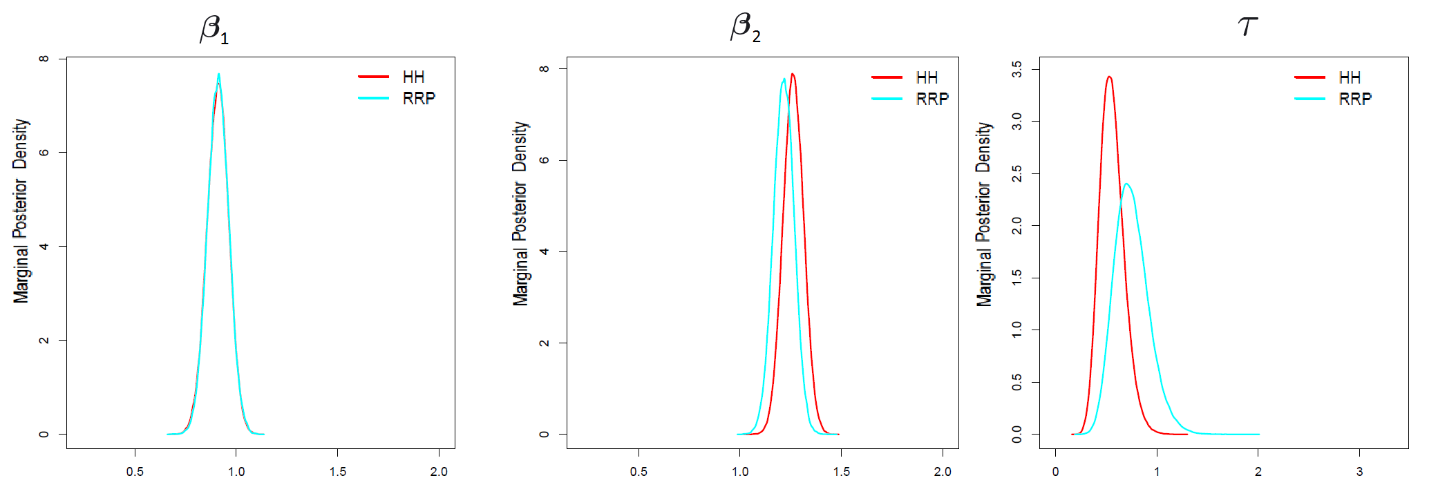
Here we compare our approach with an existing method for lattice/areal data (Hughes and Haran,, 2013). We simulate a count data set with from:
| (10) | ||||
The ICAR model has improper prior, meaning its precision matrix is rank deficient; therefore, direct simulation from (10) is not feasible. Hence, the spatial random effects is simulated using the eigencomponents of the precision matirx . Let denote the eigenpairs of , we simulate for . Then has the desired distribution. To reduce the dimension of using RRP, we will first invert using generalized inverse, then approximate using Algorithm 1 from the main text. The full conditionals of RRP for this reparameterized model can be easily derived. We then fit both RRP and HH to the simulated data set for comparison. Figure 14 shows that the marginal posterior density plot are similar from the two models.
S.5 A Comparison with Predictive Process for Point-Referenced Data
To compare the performance of our projection-based approaches with the predictive process, we simulate 100 Poisson data sets from the traditional SGLMM. We fit both FRP and RRP with rank to the datasets, and compare their results with the predictive process with reference points on a grid. In this simulation study, our projection-based approaches provide comparable inference and smaller mean prediction square error (MPSE) (Figure 15).
S.6 SGLMMs with small-scale (nugget) spatial effect
For SGLMMs where inclusion of small scale, non-spatial heterogeneity is appropriate, the model becomes,
| (11) |
where . We provide implementations of our method for two cases: (1) when Gibbs sampling of the latent variables is available, and (2) when it is not. Examples for case (1) are the spatial binary model with probit link (Berrett and Calder,, 2016, considered by) and spatial probit model for correlated ordinal data (Schliep and Hoeting,, 2015); examples for case (2) are already considered in this manuscript.
We begin by redefining some notation. Let denote the latent variable, the observed spatial binary data and the design matrix.
Case (1): We first consider the case where Gibbs sampling is available for the latent variables, for example when using SGLMM with a probit link for binary data. The model is defined as
| (12) |
where . captures large-scale spatial variation and captures small-scale variation. The conditional distribution for is therefore multivariate normal with mean and variance . Our method can be used to facilitate model fitting in this case as follows: We approximate the eigen-components of using random projections and obtain its first eigenvectors and eigenvalues . Let be the projection matrix, then we reduce the dimension of the latent variables by approximating with . For a specific value of , we can treat as fixed spatial covariates and the corresponding coefficients. Write and as the reparameterized design matrix and coefficients, respectively, then is approximated by and can be rewritten as . We use a normal conjugate prior for , inverse gamma conjugate priors for and , and a uniform prior for . Then, fitting the reduced-rank Bayesian probit model involves the following steps.
-
At the iteration of the algorithm,
-
Step 1: Gibbs update for latent variables. Sample from
- (a)
Compute projection matrix for . Form and .
- (b)
For , draw from
where is a truncated normal distribution with lower bound 0, upper bound , mean and variance .
- (a)
-
Step 2: Gibbs update for .
-
Sample from ,
-
where , and with denotes the normal prior variance.
-
-
Step 3: Gibbs update for .
-
Step 4: Gibbs update for .
-
Step 5: Metropolis-Hastings update for .
We have not provided details for steps 3-5 since they remain the same as when fitting SGLMMs in general. Furthermore, techniques for dealing with non-identifiable parameters (Berrett and Calder,, 2012, Berrett and Calder,, 2016) can also be used.
Case (2): We now consider the case where Gibbs sampling from the latent variable is not available. We first explain why the reparameterization for Case (1) is not suitable here, and then provide an alternative strategy. In Case (1) above, is reparameterized with a low-rank representation, however, the dimension of latent variable remains high; is approximated by , and has a normal distribution with mean and covariance . Constructing efficient MCMC to sample from its full conditional distribution is not easy due to its high dimensions. Hence, we propose an alternative: reduce the dimension of by approximating with , where and are eigenvectors and eigenvalues of , respectively. Hence, the eigencomponents here depend on all parameters of the covariance function. In fact is identical to from Case (1), and is identical to . This alternative reparameterization provides some computational gains. The latent variable is now approximated by whose full conditional distribution has dimensions. Reducing the dimension of the posterior distribution allows for easier construction of efficient MCMC.
References
- Adler, (1990) Adler, R. J. (1990). An introduction to continuity, extrema, and related topics for general Gaussian processes. Lecture Notes-Monograph Series, 12:i–155.
- Banerjee et al., (2012) Banerjee, A., Dunson, D. B., and Tokdar, S. T. (2012). Efficient Gaussian process regression for large datasets. Biometrika.
- Banerjee et al., (2008) Banerjee, S., Gelfand, A. E., Finley, A. O., and Sang, H. (2008). Gaussian predictive process models for large spatial data sets. Journal of the Royal Statistical Society: Series B (Statistical Methodology), 70(4):825–848.
- Belabbas and Wolfe, (2009) Belabbas, M.-A. and Wolfe, P. J. (2009). Spectral methods in machine learning and new strategies for very large datasets. Proceedings of the National Academy of Sciences, 106(2):369–374.
- Berrett and Calder, (2012) Berrett, C. and Calder, C. A. (2012). Data augmentation strategies for the Bayesian spatial probit regression model. Computational Statistics and Data Analysis, 56(3):478 – 490.
- Berrett and Calder, (2016) Berrett, C. and Calder, C. A. (2016). Bayesian spatial binary classification. Spatial Statistics, 16:72 – 102.
- Besag et al., (1991) Besag, J., York, J., and Mollié, A. (1991). Bayesian image restoration, with two applications in spatial statistics. Annals of the Institute of Statistical Mathematics, 43(1):1–20.
- Bingham and Mannila, (2001) Bingham, E. and Mannila, H. (2001). Random projection in dimensionality reduction: Applications to image and text data. In Proceedings of the seventh ACM SIGKDD international conference on Knowledge discovery and data mining, pages 245–250. ACM.
- Christensen et al., (2006) Christensen, O. F., Roberts, G. O., and Sköld, M. (2006). Robust Markov chain Monte Carlo methods for spatial generalized linear mixed models. Journal of Computational and Graphical Statistics, 15(1):1–17.
- Computational and Information Systems Laboratory, (2016) Computational and Information Systems Laboratory (2016). Yellowstone: IBM iDataPlex System (NCAR Community Computing). Boulder, CO: National Center for Atmospheric Research, http://n2t.net/ark:/85065/d7wd3xhc.
- Cressie and Johannesson, (2008) Cressie, N. and Johannesson, G. (2008). Fixed rank kriging for very large spatial data sets. Journal of The Royal Statistical Society Series B-statistical Methodology, 70:209–226.
- Cressie and Wikle, (2015) Cressie, N. and Wikle, C. K. (2015). Statistics for spatio-temporal data. John Wiley & Sons.
- Dasgupta and Gupta, (2003) Dasgupta, S. and Gupta, A. (2003). An elementary proof of a theorem of Johnson and Lindenstrauss. Random Structures & Algorithms, 22(1):60–65.
- Datta et al., (2016) Datta, A., Banerjee, S., Finley, A. O., and Gelfand, A. E. (2016). Hierarchical nearest-neighbor Gaussian process models for large geostatistical datasets. Journal of the American Statistical Association, 111(514):800–812.
- Deutsch and Wang, (1996) Deutsch, C. V. and Wang, L. (1996). Hierarchical object-based stochastic modeling of fluvial reservoirs. Mathematical Geology, 28(7):857–880.
- Diggle et al., (1998) Diggle, P. J., Tawn, J. A., and Moyeed, R. A. (1998). Model-based geostatistics. Journal of the Royal Statistical Society: Series C (Applied Statistics), 47(3):299–350.
- Drineas and Mahoney, (2005) Drineas, P. and Mahoney, M. W. (2005). On the Nyström method for approximating a Gram matrix for improved kernel-based learning. Journal of Machine Learning Research, 6(Dec):2153–2175.
- Elliott and Arbib Jr, (1953) Elliott, J. J. and Arbib Jr, R. S. (1953). Origin and status of the house finch in the Eastern United States. The Auk, pages 31–37.
- Finley et al., (2013) Finley, A. O., Banerjee, S., and Gelfand, A. E. (2013). spBayes for large univariate and multivariate point-referenced spatio-temporal data models. arXiv preprint arXiv:1310.8192.
- Finley et al., (2009) Finley, A. O., Sang, H., Banerjee, S., and Gelfand, A. E. (2009). Improving the performance of predictive process modeling for large datasets. Computational statistics & data analysis, 53(8):2873–2884.
- Flegal et al., (2008) Flegal, J. M., Haran, M., and Jones, G. L. (2008). Markov chain Monte Carlo: Can we trust the third significant figure? Statistical Science, pages 250–260.
- Frieze et al., (2004) Frieze, A., Kannan, R., and Vempala, S. (2004). Fast Monte-Carlo algorithms for finding low-rank approximations. Journal of the ACM (JACM), 51(6):1025–1041.
- Getis and Griffith, (2002) Getis, A. and Griffith, D. A. (2002). Comparative spatial filtering in regression analysis. Geographical analysis, 34(2):130–140.
- Halko et al., (2011) Halko, N., Martinsson, P.-G., and Tropp, J. A. (2011). Finding structure with randomness: Probabilistic algorithms for constructing approximate matrix decompositions. SIAM review, 53(2):217–288.
- Hanks et al., (2015) Hanks, E. M., Schliep, E. M., Hooten, M. B., and Hoeting, J. A. (2015). Restricted spatial regression in practice: Geostatistical models, confounding, and robustness under model misspecification. Environmetrics, 26(4):243–254.
- Haran, (2011) Haran, M. (2011). Gaussian random field models for spatial data. In Markov chain Monte Carlo Handbook Eds. Brooks, S.P., Gelman, A.E. Jones, G.L. and Meng, X.L., pages 449–478. Chapman and Hall/CRC.
- Haran et al., (2003) Haran, M., Hodges, J. S., and Carlin, B. P. (2003). Accelerating computation in Markov random field models for spatial data via structured MCMC. Journal of Computational and Graphical Statistics, 12:249–264.
- Harville, (1997) Harville, D. A. (1997). Matrix algebra from a statistician’s perspective. Springer, New York.
- Higdon, (1998) Higdon, D. (1998). A process-convolution approach to modelling temperatures in the North Atlantic Ocean. Environmental and Ecological Statistics, 5(2):173–190.
- Hodges and Reich, (2010) Hodges, J. S. and Reich, B. J. (2010). Adding spatially-correlated errors can mess up the fixed effect you love. The American Statistician, 64(4):325–334.
- Homrighausen and McDonald, (2016) Homrighausen, D. and McDonald, D. J. (2016). On the Nyström and column-sampling methods for the approximate principal components analysis of large datasets. Journal of Computational and Graphical Statistics, 25(2):344–362.
- Hughes and Haran, (2013) Hughes, J. and Haran, M. (2013). Dimension reduction and alleviation of confounding for spatial generalized linear mixed models. Journal of the Royal Statistical Society: Series B (Statistical Methodology), 75(1):139–159.
- John et al., (2008) John, A. K., Lake, L. W., Torres-Verdin, C., Srinivasan, S., et al. (2008). Seismic facies identification and classification using simple statistics. SPE Reservoir Evaluation & Engineering, 11(06):984–990.
- Nychka et al., (2015) Nychka, D., Bandyopadhyay, S., Hammerling, D., Lindgren, F., and Sain, S. (2015). A multiresolution Gaussian process model for the analysis of large spatial datasets. Journal of Computational and Graphical Statistics, 24(2):579–599.
- Pardieck et al., (2016) Pardieck, K. L., Ziolkowski, D. J., Hudson, M. A. R., and Campbell, K. (2016). North American breeding bird survey dataset 1966 - 2015, version 2015.0. U.S. Geological Survey, Patuxent Wildlife Research Center.
- Plummer et al., (2006) Plummer, M., Best, N., Cowles, K., and Vines, K. (2006). CODA: Convergence diagnosis and output analysis for MCMC. R News, 6(1):7–11.
- R Core Team, (2013) R Core Team (2013). R: A Language and Environment for Statistical Computing. R Foundation for Statistical Computing, Vienna, Austria.
- Rasmussen and Williams, (2005) Rasmussen, C. E. and Williams, C. K. I. (2005). Gaussian Processes for Machine Learning (Adaptive Computation and Machine Learning). The MIT Press.
- Reich et al., (2006) Reich, B. J., Hodges, J. S., and Zadnik, V. (2006). Effects of residual smoothing on the posterior of the fixed effects in disease-mapping models. Biometrics, 62(4):1197–1206.
- Rue and Held, (2005) Rue, H. and Held, L. (2005). Gaussian Markov Random Fields: Theory and Applications. CRC Press.
- Rue et al., (2009) Rue, H., Martino, S., and Chopin, N. (2009). Approximate Bayesian inference for latent Gaussian models by using integrated nested Laplace approximations. Journal of the royal statistical society: Series b (statistical methodology), 71(2):319–392.
- Sang and Huang, (2012) Sang, H. and Huang, J. Z. (2012). A full scale approximation of covariance functions for large spatial data sets. Journal of the Royal Statistical Society: Series B (Statistical Methodology), 74(1):111–132.
- Sarlos, (2006) Sarlos, T. (2006). Improved approximation algorithms for large matrices via random projections. In Proceedings of the 47th Annual IEEE Symposium on Foundations of Computer Science, FOCS ’06, pages 143–152, Washington, DC, USA. IEEE Computer Society.
- Schliep and Hoeting, (2015) Schliep, E. M. and Hoeting, J. A. (2015). Data augmentation and parameter expansion for independent or spatially correlated ordinal data. Computational Statistics and Data Analysis, 90:1 – 14.
- Sengupta and Cressie, (2013) Sengupta, A. and Cressie, N. (2013). Hierarchical statistical modeling of big spatial datasets using the exponential family of distributions. Spatial Statistics, 4(Supplement C):14 – 44.
- Sengupta et al., (2016) Sengupta, A., Cressie, N., Kahn, B. H., and Frey, R. (2016). Predictive inference for big, spatial, non-Gaussian data: Modis cloud data and its change-of-support. Australian and New Zealand Journal of Statistics, 58(1):15–45.
- Shaby and Ruppert, (2012) Shaby, B. and Ruppert, D. (2012). Tapered covariance: Bayesian estimation and asymptotics. Journal of Computational and Graphical Statistics, 21(2):433–452.
- Spiegelhalter et al., (2002) Spiegelhalter, D. J., Best, N. G., Carlin, B. P., and Van Der Linde, A. (2002). Bayesian measures of model complexity and fit. Journal of the Royal Statistical Society: Series B (Statistical Methodology), 64(4):583–639.
- Stein, (1999) Stein, M. (1999). Interpolation of Spatial Data: Some Theory for Kriging. Springer Series in Statistics. Springer New York.
- Stein, (2014) Stein, M. L. (2014). Limitations on low rank approximations for covariance matrices of spatial data. Spatial Statistics, 8(0):1 – 19. Spatial Statistics Miami.
- Tropp, (2011) Tropp, J. A. (2011). Improved analysis of the subsampled randomized Hadamard transform. Advances in Adaptive Data Analysis, 3(01n02):115–126.
- Williams and Seeger, (2001) Williams, C. and Seeger, M. (2001). Using the Nyström method to speed up kernel machines. In Advances in Neural Information Processing Systems 13, pages 682–688. MIT Press.