Quench dynamics of the three-dimensional U(1) complex field theory: geometric and scaling characterisation of the vortex tangle

Michikazu Kobayashi¹ and Leticia F. Cugliandolo^2,3 Affiliation: ¹Department of Physics, Kyoto University, Oiwake-cho, Kitashirakawa, Sakyo-ku, Kyoto 606-8502, Japan Affiliation: ²Sorbonne Universités, Université Pierre et Marie Curie - Paris 6,
Laboratoire de Physique Théorique et Hautes Energies UMR 7589, 4 Place Jussieu, 75252 Paris Cedex 05, France

August 24, 2026

Abstract

We present a detailed study of the equilibrium properties and stochastic dynamic evolution of the U(1)-invariant relativistic complex field theory in three dimensions. This model has been used to describe, in various limits, properties of relativistic bosons at finite chemical potential, type II superconductors, magnetic materials and aspects of cosmology. We characterise the thermodynamic second-order phase transition in different ways. We study the equilibrium vortex configurations and their statistical and geometrical properties in equilibrium at all temperatures. We show that at very high temperature the statistics of the filaments is the one of fully-packed loop models. We identify the temperature, within the ordered phase, at which the number density of vortex lengths falls-off algebraically and we associate it to a geometric percolation transition that we characterise in various ways. We measure the fractal properties of the vortex tangle at this threshold. Next, we perform infinite rate quenches from equilibrium in the disordered phase, across the thermodynamic critical point, and deep into the ordered phase. We show that three time regimes can be distinguished: a first approach towards a state that, within numerical accuracy, shares many features with the one at the percolation threshold, a later coarsening process that does not alter, at sufficiently low temperature, the fractal properties of the long vortex loops, and a final approach to equilibrium. These features are independent of the reconnection rule used to build the vortex lines. In each of these regimes we identify the various length-scales of the vortices in the system. We also study the scaling properties of the ordering process and the progressive annihilation of topological defects and we prove that the time-dependence of the time-evolving vortex tangle can be described within the dynamic scaling framework.

I Introduction

Three dimensional field theories with continuous symmetry breaking are relevant to describe a host of physical systems. These theories are used to model superfluid systems [1, 2, 3, 4], superconductors of type II [3, 5], nematic liquid crystals [6], magnetic samples [7], as well as phase transitions in the early universe [8].

Phase transitions with spontaneous symmetry breaking lead to the formation of topological defects of different kind: domain walls, strings or vortices, monopoles, etc. depending on the type of symmetry that is broken. The topological defects we will be interested in are line objects, be them vortices, disclinations or cosmic strings [9, 10]. These occur in, e.g., a field theory with global U(1) symmetry in $d=3$ dimensions. A field configuration has a vortex centred at a given point in space if the field vanishes at this point and the phase of the field changes by $2\pi n$ , with $n$ a non-vanishing integer, along a contour around this point. The field configuration deviates appreciably form the asymptotic value within the finite-width core of the vortex. Therefore, thin tubes of the vanishing field, i.e. the false vacuum, are enclosed within the core. This is most clearly understood in the context of liquid crystals where the orientation of the molecules rotates by such an angle when following a closed path around a line disclination [6]. Line-type topological effects are also of importance in the other branches of physics mentioned in the first paragraph. For example, topological defects were predicted to form in the Universe via the Kibble mechanism and strings were proposed to act as the source for density fluctuations at the origin of galaxy formation and other potentially observable effects [8]. They also appear in quantum turbulence [4, 11], complex-valued random wave fields [12, 13] used to model wave chaos [14] and random optical fields [12, 13].

In this paper we study the statics and stochastic dynamics of a three-dimensional relativistic field theory with global U(1) symmetry. This model serves to describe, in different limits, the physical systems mentioned in the previous paragraph as well as relativistic bosons at finite chemical potential [15, 16, 17, 18]. We mimic the coupling to an equilibrium bath by adding dissipation and noise terms in the equations of motion. We use four slightly different dynamic equations for the evolution of the fields that we call over-damped, under-damped or relativistic - the Goldstone model, ultra-relativistic, and non-relativistic - the time-dependent Gross Pitaevskii model. The resulting Langevin-like equations do not conserve the (complex) order parameter. Similar non-linear equations have been studied in the literature [19, 20, 21, 11, 22]. We show in an appendix that they lead to thermal equilibrium. We solve them with numerical methods.

The equilibrium phase diagram and critical phenomenon of the $3d$ U(1) complex field theory are well documented in the literature. In particular, the static critical exponents have been estimated with Monte Carlo simulations combined with high temperature expansions [23, 24, 25, 26], and the $\epsilon$ expansion [23, 27]. Still, we revisit the equilibrium behaviour of the system with our numerical algorithm with a double purpose. On the one hand, we validate it by showing that it takes the system to thermal equilibrium and captures the expected equilibrium properties. On the other, an important part of our analysis will be devoted to the study of the vortex tangle in, but also out of, equilibrium. As the topological stable strings must have no free ends and be closed in a space with periodic boundary conditions, we will be talking about vortex loops. We use a cubic lattice discretisation of the field theory. The construction of the vortex network on a lattice involves some ambiguity. Indeed, when a branching point at which more than one vortex line enter and exit, some criterium has to be used to decide upon the way the reconnection is done. We use here two well-documented rules [28, 29]:

– The stochastic criterium (S) in which the vortex line elements are reconnected at random.

– The maximal criterium (M) in which the vortex line elements are reconnected in such a way that one among the resulting vortex loops has the maximal possible length.

At each step of our analysis we compare the results obtained for the two rules. We pay special attention to the geometric transition between a phase in which all loops are finite, and another one in which some loops are infinitely extended. We also characterise in detail the shape and statistics of the loops on both sides of the threshold and at the geometric transition that, we show, does not coincide with the thermodynamic instability of the U(1) complex field theory. We relate the statistical properties of the closed loops in their extended phase to the one of fully-packed loop models in which each link on a lattice is covered by part of one and only one loop [30]. These configurations will be the initial states for the dynamics.

The relaxation dynamics across a second order phase transition proceeds by coarsening and annihilation of topological defects [31, 32]. Analytic approximations to characterize the scaling properties of the relaxation dynamics of models with continuous symmetry, after an infinitely rapid quench into the ordered phase, were developed in [36, 34, 37, 33, 35], see [31] for a review. The dynamic exponent $z_{\mathrm{d}}=2$ was predicted analytically [36, 34, 33, 35, 37], and a value close to this analytic prediction was measured numerically [39, 38, 40] and experimentally in bulk nematic liquid crystals [41, 42] from the analysis of space-time correlation functions and dynamic structure factors. As far as we know, there is no detailed study of the dynamics from the point of view of the topological defects themselves and we also develop it here.

Some details about the methodology that we use to investigate this problem are in order. In the analysis of the phase transition and static vortex statistics we ensure that the system reaches thermal equilibrium. In the analysis of the evolution after a deep instantaneous quench below the ordering transition temperature we simply let the system evolve from a chosen initial state under subcritical conditions. The vortex string network already present in the initial state evolves after the quench and we characterise its evolution in full detail. We identify various dynamic regimes and we explain what determines them in terms of the changing vortex configurations. We base this analysis on the work in [43, 44, 45, 47, 46, 48, 49, 50, 51, 52, 53, 54] where the stochastic ordering dynamics of $2d$ spin models were analysed from a geometric perspective.

The paper is organised as follows. In Sec. II we introduce the model. In Sec. III we describe the equilibrium properties and phase transition in the model; it can be read independently from the rest of the paper. In Sec IV we discuss the properties of the vortex network in equilibrium. Section V is devoted to the analysis of the fast quench dynamics. Finally, in Sec. VI we present our conclusions and some lines for future research. A short account of some of our results appeared in [55].

II The model

The Lagrangian density for relativistic bosons with finite chemical potential reads [56], in terms of a scalar complex field $\psi$ and its time derivative $\dot{\psi}=\partial_{t}\psi$ ,

\displaystyle\begin{split}&\mathcal{L}[\dot{\psi}(\bm{x},t),\dot{\psi}^{\ast}(\bm{x},t),\psi(\bm{x},t),\psi^{\ast}(\bm{x},t)]\\ &\qquad=\frac{1}{c^{2}}|\dot{\psi}(\bm{x},t)|^{2}+i\mu\{\psi^{\ast}(\bm{x},t)\dot{\psi}(\bm{x},t)-\dot{\psi}^{\ast}(\bm{x},t)\psi(\bm{x},t)\}-|\nabla\psi(\bm{x},t)|^{2}\\ &\qquad\quad+g\rho|\psi(\bm{x},t)|^{2}-\frac{g}{2}|\psi(\bm{x},t)|^{4},\end{split}

(1)

where $c$ is the speed of light and $g$ and $\rho$ are real parameters, $g,\rho\in\mathbb{R}$ , in the potential energy density with Mexican hat form and a degenerate circle of minima at $|\psi|^{2}=\rho$ . The parameters $\mu\in\mathbb{R}$ and $\rho$ receive different interpretations in different communities. The term proportional to $\mu$ breaks the particle-antiparticle symmetry and in the high-energy literature it is associated to a chemical potential, while $\rho$ fixes the vacuum expectation value of the U(1) symmetry breaking. In the condensed matter literature instead the chemical potential is associated to $\rho$ that fixes the particle density $|\psi|^{2}$ in the system and $\mu$ is related to the mass of the particles.

This theory is global U(1)-invariant as the Lagrangian density remains unchanged under the global transformation, $\psi^{\prime}(\bm{x},t)=e^{i\delta}\psi(\bm{x},t)$ , and accordingly for $\psi^{*}$ , with $\delta$ a space and time independent real parameter. Moreover, $\mathcal{L}^{*}=\mathcal{L}$ .

The Lagrangian density (1) is also invariant under the Lorentz boost

\displaystyle\begin{split}&t^{\prime}=\gamma_{c}\bigg(t-\frac{\bm{v}\cdot\bm{x}}{c^{2}}\bigg),\quad\qquad\bm{x}^{\prime}=\bm{x}-\bm{v}\left[\frac{(1-\gamma_{c})}{v^{2}}(\bm{v}\cdot\bm{x})+\gamma_{c}t\right],\end{split}

(2)

with Lorentz factor $\gamma_{c}=(1-v^{2}/c^{2})^{-1/2}$ , if the field transforms as

\displaystyle\begin{split}&\psi^{\prime}(\bm{x}^{\prime},t^{\prime})=\exp\bigg[-i\mu c^{2}\bigg\{(1-\gamma_{c})t+\frac{\gamma_{c}\bm{v}\cdot\bm{x}}{c^{2}}\bigg\}\bigg]\psi(\bm{x},t).\end{split}

(3)

Indeed, under these transformations, $\mathcal{L}[\partial_{t}{\psi}(\bm{x},t),\partial_{t}{\psi}^{\ast}(\bm{x},t),\psi(\bm{x},t),\psi^{\ast}(\bm{x},t)]=$ $\mathcal{L}[\partial_{t^{\prime}}\psi^{\prime}(\bm{x}^{\prime},t^{\prime}),\partial_{t^{\prime}}{\psi^{\prime}}^{\ast}(\bm{x}^{\prime},t^{\prime}),\psi^{\prime}(\bm{x}^{\prime},t^{\prime}),\psi^{\prime\ast}(\bm{x}^{\prime},t^{\prime})]$ . The inverse transformations are $t=\gamma_{c}(t^{\prime}+\bm{v}\cdot\bm{x}^{\prime}/c^{2})$ and $\bm{x}=\bm{x}^{\prime}+\bm{v}\left[\gamma_{c}t^{\prime}-(1-\gamma_{c})(\bm{v}\cdot\bm{r}^{\prime})/v^{2}\right]$ and these imply

\displaystyle\begin{split}\partial_{t^{\prime}}=\gamma_{c}(\partial_{t}+\bm{v}\cdot\nabla),\quad\qquad\nabla^{\prime}=\nabla-\bm{v}\left[\frac{(1-\gamma_{c})}{v^{2}}(\bm{v}\cdot\nabla)+\frac{\gamma_{c}}{c^{2}}\partial_{t}\right].\end{split}

(4)

The equation of motion for $\psi$ follows from the Euler-Lagrangian equation and reads

\displaystyle-\bigg(\frac{1}{c^{2}}\frac{\partial^{2}}{\partial t^{2}}-\nabla^{2}\bigg)\psi+2i\mu\dot{\psi}\equiv-\Box\psi+2i\mu\dot{\psi}=g(|\psi|^{2}-\rho)\psi.

(5)

We consider two opposite limits: $\mu\to 0$ and $c\to\infty$ . In the former case, the complex field $\psi$ does not change under the Lorentz transformation (3), and we call it the “ultra-relativistic” limit. The latter case is “non-relativistic”. Under these two limits, Eq. (5) becomes


$\displaystyle-\Box\psi$	$\displaystyle=g(\|\psi\|^{2}-\rho)\psi,\qquad\qquad\qquad\qquad\mu\to 0,$	(6a)
$\displaystyle 2i\mu\dot{\psi}$	$\displaystyle=-\nabla^{2}\psi+g(\|\psi\|^{2}-\rho)\psi,\qquad\qquad c\to\infty,$	(6b)

which are known as the Goldstone and the Gross-Pitaevskii models respectively. The latter describes the dynamics of gaseous Bose-Einstein condensates [2]. The former, on the other hand, describes the dynamics of condensates in optical lattices which are close to the critical point to the Mott insulator phase with integer fillings [57].

Under the time evolution in Eq. (5), the energy functional

\displaystyle E(\dot{\psi},\dot{\psi}^{\ast},\psi,\psi^{\ast})=\int d\bm{x}\>\bigg\{\frac{|\dot{\psi}|^{2}}{c^{2}}+|\nabla\psi|^{2}-g\rho|\psi|^{2}+\frac{g}{2}|\psi|^{4}\bigg\}

(7)

is conserved.

The static solutions to (5) that minimize the energy are $\psi=\sqrt{\rho}\ e^{i\chi}$ with $\chi$ a constant. The choice of $\chi$ breaks the U(1) symmetry. Vortex static solutions are also supported by this equation [21, 11]. One such $z$ -directed string is given by the axisymmetric field configuration $\psi(\bm{x})=f(r)e^{in\theta}$ with $f(r)$ a smooth function of $r$ , the radial direction on the plane perpendicular to the tube. It takes the extreme values $f(0)=0$ and $f(r\to\infty)=\sqrt{\rho}$ and varies over a typical length scale $\simeq(g\rho)^{-1/2}$ that determines the core of the vortex. $n$ is the winding number.

Next, we consider the statistical properties of the system described by the U(1) complex field at finite temperatures. In canonical equilibrium the statistical average of a real finite functional of the fields $f=f(\psi,\psi^{\ast},\dot{\psi},\dot{\psi}^{\ast})$ reads

\displaystyle\begin{split}\langle f\rangle_{\mathrm{eq}}&\equiv\int D\dot{\psi}\>D\dot{\psi}^{\ast}\>D\psi\>D\psi^{\ast}\>f\ \frac{e^{-E/T}}{Z},\\ Z&=\int D\dot{\psi}\>D\dot{\psi}^{\ast}\>D\psi\>D\psi^{\ast}\>e^{-E/T},\end{split}

(8)

where $T$ is temperature. We set the Boltzmann constant to $k_{\mathrm{B}}=1$ in this paper. When $f$ depends only on $\psi$ and $\psi^{\ast}$ , i.e., $f(\psi,\psi^{\ast},\dot{\psi},\dot{\psi}^{\ast})\to f(\psi,\psi^{\ast})$ , Eq. (8) can be simplified to

\displaystyle\begin{split}\langle f\rangle_{\mathrm{eq}}&=\int D\psi\>D\psi^{\ast}\>f\ \frac{e^{-E_{0}/T}}{Z_{0}},\\ Z_{0}&=\int D\psi\>D\psi^{\ast}\>e^{-E_{0}/T},\end{split}

(9)

with

E_{0}(\psi,\psi^{\ast})=\int d\bm{x}\>\bigg\{|\nabla\psi|^{2}-g\rho|\psi|^{2}+\frac{g}{2}|\psi|^{4}\bigg\}.

(10)

These are the kind of functionals that we consider in this paper, unless we specify a different dependence.

At $T=0$ the ground state is $|\psi|^{2}=\rho$ and the U(1) symmetry of the energy functional $E_{0}$ for the phase shift of $\psi$ is spontaneously broken. We therefore expect the temperature at which the spontaneous breaking of this symmetry occurs to be the one for Bose-Einstein condensation.

A simple and efficient method to sample the thermal averages defined above is to use the over-damped Langevin equation

\displaystyle\begin{split}&\gamma_{\mathrm{L}}\dot{\psi}=-\frac{\delta E_{0}}{\delta\psi^{\ast}}+\sqrt{\gamma_{\mathrm{L}}T}(\xi_{1}+i\xi_{2})=\nabla^{2}\psi-g(|\psi|^{2}-\rho)\psi+\sqrt{\gamma_{\mathrm{L}}T}(\xi_{1}+i\xi_{2}),\\ &\langle\xi_{a}(\bm{x},t)\rangle=0,\qquad\langle\xi_{a}(\bm{x},t)\xi_{b}(\bm{x}^{\prime},t^{\prime})\rangle=\delta(t-t^{\prime})\delta(\bm{x}-\bm{x}^{\prime})\delta_{a,b},\end{split}

(11)

that ensures

\displaystyle\frac{1}{t}\int_{0}^{t}dt^{\prime}\>f[\psi(\bm{x},t^{\prime}),\psi^{\ast}(\bm{x},t^{\prime})]\stackrel{{\scriptstyle t\to\infty}}{{\longrightarrow}}\langle f\rangle_{\mathrm{eq}}.

(12)

An alternative dynamic approach uses, instead of the energy functional in Eq. (7), the Hamiltonian associated to the Lagrangian density (1)

\displaystyle\begin{split}&H(\psi,\psi^{\ast},\phi,\phi^{\ast})=\int d\bm{x}\>\bigg\{c^{2}(\phi^{\ast}-i\mu\psi^{\ast})(\phi+i\mu\psi)+|\nabla\psi|^{2}-g\rho|\psi|^{2}+\frac{g}{2}|\psi|^{4}\bigg\}\\ &\phantom{H(\psi,\psi^{\ast},\phi,\phi^{\ast})}=E_{0}(\psi,\psi^{\ast})+c^{2}\int d\bm{x}\>(\phi^{\ast}-i\mu\psi^{\ast})(\phi+i\mu\psi)\end{split}

(13)

with the generalized momentum $\phi$

\displaystyle\begin{split}&\phi=\frac{\partial\mathcal{L}}{\partial\dot{\psi}^{\ast}}=\frac{\dot{\psi}}{c^{2}}-i\mu\psi,\end{split}

(14)

and its complex conjugate $\phi^{*}$ . The under-damped Langevin equation

\displaystyle\begin{split}\dot{\phi}=-\frac{\delta H}{\delta\psi^{\ast}}-\gamma_{\mathrm{L}}c^{2}(\phi+i\mu\psi)+\sqrt{\gamma_{\mathrm{L}}T}(\xi_{1}+i\xi_{2})\end{split}

(15)

becomes

\displaystyle\begin{split}-\Box\psi+(2i\mu-\gamma_{\mathrm{L}})\dot{\psi}=g(|\psi|^{2}-\rho)\psi-\sqrt{\gamma_{\mathrm{L}}T}(\xi_{1}+i\xi_{2}).\end{split}

(16)

See Refs. [58] for an alternative derivation of the dissipative term proportional to $-\gamma_{\mathrm{L}}\dot{\psi}$ . In the ultra-relativistic and non-relativistic limits, the Langevin equation (16) approaches


$\displaystyle-\Box\psi$	$\displaystyle=g(\|\psi\|^{2}-\rho)\psi+\gamma_{\mathrm{L}}\dot{\psi}-\sqrt{\gamma_{\mathrm{L}}T}(\xi_{1}+i\xi_{2}),$	(17a)
$\displaystyle(2i\mu-\gamma_{\mathrm{L}})\dot{\psi}$	$\displaystyle=-\nabla^{2}\psi+g(\|\psi\|^{2}-\rho)\psi-\sqrt{\gamma_{\mathrm{L}}T}(\xi_{1}+i\xi_{2}).$	(17b)

Equation (17a) is the conventional under-damped Langevin equation corresponding to the over-damped Langevin equation (11), whereas Eq. (17b) is known as the stochastic Gross-Pitaevskii equation describing Bose-Einstein condensates at finite temperatures [17]. The Hamiltonian (14) and the Langevin equation (16) give the same ensemble averages for equilibrium states as those obtained using Eqs. (7) and (10),

\displaystyle\begin{split}\langle f\rangle_{\mathrm{eq}}&=\int D\psi\>D\psi^{\ast}\>D\phi\>D\phi^{\ast}\>f\ \frac{e^{-H/T}}{Z_{H}}=\int D\psi\>D\psi^{\ast}\>f\ \frac{e^{-E_{0}/T}}{Z_{0}},\\ Z_{H}&=\int D\psi\>D\psi^{\ast}\>D\phi\>D\phi^{\ast}\>e^{-H/T},\end{split}

(18)

see App. A.

Although the above discussion applies in all dimensions, we concentrate in three-dimensional systems in this paper. We close this section by making explicit the numerical procedure that we used to solve eqs. (11), (16), (17a), and (17b) numerically. We first collect time and space coordinates into a four component vector that we call $\mbox{\bf x}=(x_{0},x_{1},x_{2},x_{3})$ with $x_{0}=t$ and $\bm{x}=(x_{1},x_{2},x_{3})$ the space-like components. We discretize x using a different mesh in the space and time directions: $x_{1}=j\Delta x$ with $j=0,\dots,L-1$ , $x_{2}=k\Delta x$ with $k=0,\dots,L-1$ , $x_{3}=l\Delta x$ with $l=0,\dots,L-1$ , and $x_{0}=i\Delta t$ with $i=0,\dots$ We define the complex field $\psi$ on the discretised space-time as $\psi_{\mbox{\bf x}}\equiv\psi(t,\bm{x})$ with $\mbox{\bf x}\equiv(i\Delta t,j\Delta x,k\Delta x,l\Delta x)$ . We call $\hat{e}_{0},\hat{e}_{1},\hat{e}_{2},\hat{e}_{3}$ the orthonormal basis of unit vectors on the vector x. The spatial gradient then becomes

	$\displaystyle\|\nabla\psi\|^{2}$	$\displaystyle\to\sum_{a=1}^{3}\frac{\|\psi_{\mbox{\bf x}}-\psi_{\mbox{\bf x}-\Delta x\hat{e}_{a}}\|^{2}}{(\Delta x)^{2}},$		(19)
	$\displaystyle\nabla^{2}\psi$	$\displaystyle\to\sum_{a=1}^{3}\frac{\psi_{\mbox{\bf x}+\Delta x\hat{e}_{a}}+\psi_{\mbox{\bf x}-\Delta x\hat{e}_{a}}-2\psi_{\mbox{\bf x}}}{(\Delta x)^{2}},$		(20)

and the spatial integral $\int d\bm{x}\>\to(\Delta x)^{3}\sum_{j,k,l}$ , with $\Delta x$ the lattice spacing. We use periodic cubes with linear sizes $L=40$ , $60$ , $80$ , and $100$ . For the time evolution, we use the lowest-ordered stochastic Runge-Kutta method for Eq. (11),

\displaystyle\begin{split}&\psi_{(1)\mbox{\bf x}}=\psi_{\mbox{\bf x}}-\frac{\partial E_{0}[\psi_{\mbox{\bf x}},\psi^{\ast}_{\mbox{\bf x}}]}{\partial\psi^{\ast}_{\mbox{\bf x}}}\frac{\Delta t}{\gamma_{\mathrm{L}}}+\sqrt{\frac{T\Delta t}{\gamma_{\mathrm{L}}}}(\Delta W_{\mbox{\bf x},1}+i\Delta W_{\mbox{\bf x},2}),\\ &\psi_{(2)\mbox{\bf x}}=\psi_{\mbox{\bf x}}-\frac{\partial E_{0}[\psi_{\mbox{\bf x}},\psi^{\ast}_{\mbox{\bf x}}]}{\partial\psi^{\ast}_{\mbox{\bf x}}}\frac{\Delta t}{2\gamma_{\mathrm{L}}}+\sqrt{\frac{T\Delta t}{\gamma_{\mathrm{L}}}}(\Delta W_{\mbox{\bf x},1}+i\Delta W_{\mbox{\bf x},2}),\\ &\psi_{\mbox{\bf x}+\Delta t\hat{e}_{0}}=\psi_{(2)\mbox{\bf x}}-\frac{\partial E_{0}[\psi_{(1)\mbox{\bf x}},\psi_{(1)\mbox{\bf x}}^{\ast}]}{\partial\psi_{(1)\mbox{\bf x}}^{\ast}}\frac{\Delta t}{2\gamma_{\mathrm{L}}},\end{split}

(21)

and for Eq. (17b),

\displaystyle\begin{split}&\psi_{(1)\mbox{\bf x}}=\psi_{\mbox{\bf x}}+\frac{\partial E_{0}[\psi_{\mbox{\bf x}},\psi^{\ast}_{\mbox{\bf x}}]}{\partial\psi^{\ast}_{\mbox{\bf x}}}\frac{\Delta t}{2i\mu-\gamma_{\mathrm{L}}}+\frac{\displaystyle\sqrt{\gamma_{\mathrm{L}}T\Delta t}}{2i\mu-\gamma_{\mathrm{L}}}(\Delta W_{\mbox{\bf x},1}+i\Delta W_{\mbox{\bf x},2}),\\ &\psi_{(2)\mbox{\bf x}}=\psi_{\mbox{\bf x}}+\frac{\partial E_{0}[\psi_{\mbox{\bf x}},\psi^{\ast}_{\mbox{\bf x}}]}{\partial\psi^{\ast}_{\mbox{\bf x}}}\frac{\Delta t}{2(2i\mu-\gamma_{\mathrm{L}})}+\frac{\displaystyle\sqrt{\gamma_{\mathrm{L}}T\Delta t}}{2i\mu-\gamma_{\mathrm{L}}}(\Delta W_{\mbox{\bf x},1}+i\Delta W_{\mbox{\bf x},2}),\\ &\psi_{\mbox{\bf x}+\Delta t\hat{e}_{0}}=\psi_{(2)\mbox{\bf x}}+\frac{\partial E_{0}[\psi_{(1)\mbox{\bf x}},\psi_{(1)\mbox{\bf x}}^{\ast}]}{\partial\psi_{(1)\mbox{\bf x}}^{\ast}}\frac{\Delta t}{2(2i\mu-\gamma_{\mathrm{L}})},\end{split}

(22)

and the lowest-ordered symplectic method for Eq. (17a)

\displaystyle\begin{split}&\psi_{\mbox{\bf x}+\Delta t\hat{e}_{0}}=\psi_{\mbox{\bf x}}+c^{2}\phi_{\mbox{\bf x}}\Delta t,\\ &\phi_{\mbox{\bf x}+\Delta t\hat{e}_{0}}=\phi_{\mbox{\bf x}}-\bigg(\frac{\partial E_{0}[\psi_{\mbox{\bf x}},\psi^{\ast}_{\mbox{\bf x}}]}{\partial\psi^{\ast}_{\mbox{\bf x}}}+c^{2}\gamma_{\mathrm{L}}\phi_{\mbox{\bf x}}\bigg)\Delta t+\sqrt{\gamma_{\mathrm{L}}T\Delta t}(\Delta W_{\mbox{\bf x},1}+i\Delta W_{\mbox{\bf x},2}),\end{split}

(23)

and for Eq. (16),

\displaystyle\begin{split}&\psi_{\mbox{\bf x}+\Delta t\hat{e}_{0}}=\psi_{\mbox{\bf x}}+c^{2}\phi_{\mbox{\bf x}}\Delta t,\\ &\phi_{\mbox{\bf x}+\Delta t\hat{e}_{0}}=\phi_{\mbox{\bf x}}-\bigg\{\frac{\partial E_{0}[\psi_{\mbox{\bf x}},\psi^{\ast}_{\mbox{\bf x}}]}{\partial\psi^{\ast}_{\mbox{\bf x}}}+c^{2}(\gamma_{\mathrm{L}}-2i\mu)\phi_{\mbox{\bf x}}\bigg\}\Delta t\\ &\phantom{\phi_{\mbox{\bf x}+\Delta t\hat{e}_{0}}=}+\sqrt{\gamma_{\mathrm{L}}T\Delta t}(\Delta W_{\mbox{\bf x},1}+i\Delta W_{\mbox{\bf x},2}),\end{split}

(24)

with $\langle\Delta W_{\mbox{\bf x},a}\rangle=0$ and $\langle\Delta W_{\mbox{\bf x},a}\Delta W_{\mbox{\bf x}^{\prime},b}\rangle=\delta_{\mbox{\bf x},\mbox{\bf x}^{\prime}}\delta_{a,b}$ . As regards the numerical parameters, we use $c=1$ , $\rho=1$ , $g=1$ , $\mu=0.5$ , $\gamma_{\mathrm{L}}=1$ , $\Delta x=1$ in all cases, and $\Delta t=0.005$ for Eq. (21) and $\Delta t=0.01$ for Eqs. (22), (23), and (24). The number of spatial grid points is $N=L^{3}$ . With these parameters, space and time are measured in units of the equilibrium correlation length at $T=0$ in the mean-field approximation, $x_{0}\equiv 1/\sqrt{g\rho}$ , and the corresponding correlation time $t_{0}\equiv\gamma_{\mathrm{L}}/x_{0}^{2}$ . The order parameter is further measured in units of $\sqrt{\rho}$ with $\rho$ the zero-temperature density. Then the velocity $c$ , parameter $\mu$ , temperature $T$ , and the Langevin noise $\xi_{a}$ are measured in units of $x_{0}/t_{0}$ , $t_{0}/x_{0}^{2}$ , $x_{0}^{-2}$ , and $\sqrt{\rho/t_{0}}$ , respectively.

III Equilibrium properties

In this section, we focus on the equilibrium properties attained by the dynamical model. As we will show, this model undergoes a second order phase transition at a critical point below which the U(1) continuous symmetry is spontaneously broken. We confirm numerically that the universality class it the same as the one of the usual U(1) complex field theory [59, 60, 61]. This critical phenomenon has been studied with equilibrium methods in the past and the best estimates for the critical exponents are [24]

\displaystyle\begin{array}[]{llll}&\alpha=-0.0151(3),&\nu=0.6717(1),&\eta=0.0381(2),\\ &\gamma=1.3178(2),&\beta=0.3486(1),&\delta=4.780(1).\end{array}

These have been obtained with finite-size scaling of Monte Carlo data for system sizes up to $L=128$ and high-temperature expansions. The $\epsilon$ -expansion RG method yields [27]

\displaystyle\begin{array}[]{llll}&\alpha=-0.011(4),&\nu=0.6703(15),&\eta=0.0354(25),\\ &\gamma=1.3169(20),&\beta=0.3470(16),&\delta=4.795(14).\end{array}

These values are compatible with the ones given above within numerical error and also with other numerical evaluations [26]. Since, the spontaneous breaking of the U(1) symmetry is isomorphic to the one in the $3d$ $XY$ -spin model, these critical exponents are expected to be the same as the ones of this spin model. Experimental measurements in the superfluid transition of ⁴He yield $\alpha=-0.0127(3)$ [62]. Other experimental results for this and other critical exponents can be found in [23]. The dynamic critical exponent $z_{\rm eq}$ was estimated to be $z_{\rm eq}\simeq 2.1$ for periodic boundary conditions with numerical methods in [63, 64], see also [61] for the RG prediction, and we will further discuss it below.

Our aim in this section is twofold. On the one hand, we test whether the three dynamic formulations, given by the Langevin equations (11), and (16) in its two limits (17), capture the equilibrium and critical phenomena correctly. In order to avoid long relaxation times and reach equilibrium more quickly, we start all simulations from the completely ordered initial state $\psi(t=0)=\sqrt{\rho}$ . We estimate the relaxation time to be $\tau\lesssim 900$ for the parameters explored, and we verify that the system reaches its asymptotic regime for $t>1000$ , see Fig. 8. On the other hand, we characterize the equilibrium configurations at off-critical and critical temperatures. We confirm that the percolation of the longest vortex loops in equilibrium occurs at a temperature that is within the ordered phase and different from the critical one [28, 29, 55]. We pay special attention to the geometric and statistical properties of the vortex lines at the critical percolation point, as these are going to be of relevance to our analysis of the relaxation dynamics. We also distinguish the statistical and geometrical properties of the string networks obtained with the two reconnection conventions.

In this section, we perform a double average of data: we take an ensemble average by taking the mean over $100$ noise realisations for the same initial state $\psi(t=0)=\sqrt{\rho}$ , and we average over $3000$ different times at $t=(1000+i)\Delta t$ with $1\leq i\leq 3000$ for each dynamical run. The total number of data contributing to each data point shown is, therefore, $100\times 3000$ . We write this ensemble average as $\langle\cdots\rangle_{\mathrm{stat}}$ and we use this as the equilibrium ensemble average $\langle\cdots\rangle_{\mathrm{eq}}$ . The lattice linear sizes used are comparable to the ones utilized in Monte Carlo studies of the phase transition and critical phenomena [24].

Refer to caption — Figure 1: (Color online.) Temperature dependence of the order parameter $m$ . (a) Comparison between the estimate for $m(T)$ obtained with different stochastic dynamics: over-damped Langevin equation (11) (over), under-damped Langevin equation (16) (rel), ultra-relativistic limit of the under-damped Langevin equation (17a) (untra-rel), and non-relativistic limit of the under-damped Langevin equation (17b) (non-rel). Systems with $L=100$ linear size are used in all cases. (b) Finite size dependence of $m(T)$ as obtained from the under-damped Langevin equation (16). In both panels, we plot with a dotted line the critical decay of the order parameter, $m(T)\propto(T_{\mathrm{c}}-T)^{\beta}$ , at temperatures $T<T_{\mathrm{c}}$ with $T_{\mathrm{c}}=2.26$ and $\beta=0.347$ . For details on these values see Figs. 2 and 4 (a), and the corresponding discussion. In the inserts: zoom over the critical region.

III.1 The order parameter

There are three well-known definitions of the order parameter $m$ for the spontaneous breaking of the U(1) symmetry. In the usual one is statistical physics, $m$ is calculated as $m\equiv\lim_{h\to 0}\langle\psi_{h}\rangle_{\mathrm{eq}}$ by applying a perturbation $h$ that couples linearly to the field. In the case of the model with Hamiltonian $H$ this is achieved as

\displaystyle H=E_{0}(\psi_{h},\psi^{\ast}_{h})+c^{2}\int d\bm{x}\>\{(\phi^{\ast}_{h}-i\mu\psi^{\ast}_{h})(\phi_{h}+i\mu\psi_{h})-h(\psi_{h}+\psi^{\ast}_{h})\},

(31)

where the sub-index _h recalls that the complex fields $\psi_{h}$ and $\phi_{h}$ are computed under the external field $h$ . The resulting Langevin equation becomes

\displaystyle\begin{split}-\Box\psi_{h}+(2i\mu-\gamma_{\mathrm{L}})\dot{\psi}_{h}=g(|\psi_{h}|^{2}-\rho)\psi_{h}-h-\sqrt{\gamma_{\mathrm{L}}T}(\xi_{1}+i\xi_{2}).\end{split}

(32)

In the context of Bose-Einstein condensation and superfluidity, however, the external field $h$ does not find an easy implementation and, instead, the following definition is considered:

\displaystyle m\propto\sqrt{|C(r\to\infty)|},\quad C(r)=\Bigg\langle\frac{1}{4\pi r^{2}}\int d\Omega_{\bm{r}=r}\>\int d\bm{x}\>\psi^{\ast}(\bm{x})\psi(\bm{x}+\bm{r})\Bigg\rangle_{\mathrm{eq}},

(33)

where the integral $1/(4\pi r^{2})\int d\Omega_{\bm{r}=r}$ is the average over the solid angle at $\bm{r}=r$ . Numerically, $m$ is computed as $m\propto\sqrt{|C(r=L/2)|}$ , and in order to improve the numerical accuracy of the measurement of the integral over the spherical surface, $1/(4\pi r^{2})\int d\Omega_{\bm{r}=r}$ , we average over all lattice sites falling within the shell $[|\bm{r}|,|\bm{r}|+1)$ . This definition corresponds to the off-diagonal long-range order $\lim_{\bm{r}\to\infty}\langle\psi^{\dagger}(\bm{x})\psi(\bm{x}+\bm{r})\rangle$ for the presence of the Bose-Einstein condensate in a quantum-boson system.

In many numerical works, the definition

\displaystyle m\equiv\big\langle\big|\overline{\psi}\big|\big\rangle_{\mathrm{eq}},\quad\qquad\overline{\psi}=\frac{1}{L^{3}}\sum_{j,k,l}\psi_{\mbox{\bf x}}.

(34)

is instead used due to its numerical simplicity.

All definitions of $m$ should give the same temperature dependence for sufficiently large system size $L$ . We adopt the definition (34) in this paper.

Figure 1 shows the temperature dependence of the order parameter, $m$ , for the spontaneous breaking of the U(1) symmetry for different Langevin equations [Fig. 1 (a)] and for different system sizes $L$ [Fig. 1 (b)]. Different Langevin equations give the same ensemble averages, within numerical accuracy. From this figure, we roughly calculate that the spontaneous symmetry breaking occurs at $T_{\mathrm{c}}\simeq 2.3$ in the $L\to\infty$ limit. The dotted blue lines in both panels represent the critical behaviour, $m(T)\simeq|T-T_{c}|^{\beta}$ with $T_{c}=2.26$ [see Eq. (36)] and $\beta=0.347$ . They are very close to the numerical results. In the inset we zoom over the critical region.

We end with a note on the difference between $m$ and the particle number observable, $L^{-3}\sum_{jkl}|\psi_{\mbox{\bf x}}|$ , that is different from zero at all $T$ (see the inset in Fig. 1 in [55]).

III.2 The critical temperature

The critical temperature can be better evaluated from the Binder ratio, $U_{1}$ , and the ratio of correlation functions, $U_{2}$ ,

\displaystyle U_{1}\equiv\frac{\displaystyle\big\langle\big|\overline{\psi}\big|^{4}\big\rangle_{\mathrm{eq}}}{\displaystyle\big\langle\big|\overline{\psi}\big|^{2}\big\rangle_{\mathrm{eq}}^{2}},\qquad\qquad\qquad U_{2}\equiv\frac{C(r=L/2)}{C(r=L/4)}.

(35)

$U_{1}$ and $U_{2}$ are expected to take fixed values independently of the system size $L$ at the critical temperature $T_{\mathrm{c}}$ .

Figure 2 shows the temperature dependence of $U_{1}$ (a) and $U_{2}$ (b) obtained from the under-damped Langevin equation (16). The estimated critical temperature is

T_{\mathrm{c}}=2.26\pm 0.02\;.

(36)

As well as for $m$ , the other Langevin equations (11), (17a), and (17b) give almost the same values of $U_{1}$ , $U_{2}$ and $T_{\mathrm{c}}$ (not shown).

We also calculated the susceptibility

\displaystyle\chi\equiv\frac{\displaystyle\big\langle\big|\overline{\psi}\big|^{2}\big\rangle_{\mathrm{eq}}-\big\langle\big|\overline{\psi}\big|\big\rangle_{\mathrm{eq}}^{2}}{T}

(37)

and the specific heat

\displaystyle C\equiv\frac{d\langle E_{0}\rangle_{\mathrm{eq}}}{dT},

(38)

that assuming the equilibrium ensemble average shown in Eq. (10), can also be written as

\displaystyle C=\frac{\langle E_{0}^{2}\rangle_{\mathrm{eq}}-\langle E_{0}\rangle_{\mathrm{eq}}^{2}}{T^{2}}.

(39)

We implemented these definitions numerically as

\displaystyle C_{1}\equiv\frac{\langle E_{0}^{2}\rangle_{\mathrm{stat}}-\langle E_{0}\rangle_{\mathrm{stat}}^{2}}{T^{2}},\quad C_{2}\equiv\frac{\langle E_{0}(T+\Delta T)\rangle_{\mathrm{stat}}-\langle E_{0}(T-\Delta T)\rangle_{\mathrm{stat}}}{2\Delta T}.

(40)

The equilibrium correlation length $\xi_{\mathrm{eq}}$ was calculated by assuming that the connected correlation length decays exponentially as $C(r)-m^{2}\to r^{-r/\xi_{\mathrm{eq}}}$ , from the corresponding small- $k$ behaviour or the structure factor

S(k)\equiv\Bigg\langle\frac{1}{4\pi k^{2}L^{3}}\int d\Omega_{\bm{k}=k}\>|\tilde{\psi}(\bm{k})|^{2}\Bigg\rangle_{\mathrm{eq}},

(41)

with $\tilde{\psi}(\bm{k})=\int d\bm{x}\>\psi(\bm{x})e^{-i\bm{k}\cdot\bm{x}}$ the Fourier transformation of the field, estimated numerically from

\displaystyle\frac{S(k=2\pi/\xi_{\mathrm{eq}})}{S(k\to 0)}=10^{-1},\quad S(k\to 0)\equiv 2S(\Delta k)-S(2\Delta k),

(42)

where $S(k\to 0)$ is the linear interpolation from $S(\Delta k)$ and $S(2\Delta k)$ to the value at $k=0$ with $\Delta k=2\pi/L$ .

The panels (a)-(d) in Fig. 3 show the temperature dependences of $\chi$ , $C_{1}$ , $C_{2}$ , and $\xi_{\mathrm{eq}}$ for $L=100$ . Their values are also almost independent of the type of Langevin equation used even close to criticality at $T\simeq T_{c}$ . The two specific heats $C_{1}$ and $C_{2}$ are almost the same except for the slightly more jagged shape of $C_{1}$ . We note that both $C_{1}$ and $C_{2}$ converge to the finite values $C_{1}\simeq 1$ and $C_{2}\simeq 1$ in the zero temperature limit, because of the continuous U(1) symmetry breaking and the resulting Nambu-Goldstone modes. This unphysical result can be cured by taking into account quantum effects.

III.3 Critical scaling

Finite-size scaling [65] states that $m/L^{-\beta/\nu}$ , $\chi/L^{\gamma/\nu}$ , $C_{1}/L^{\alpha/\nu}$ , $C_{2}/L^{\alpha/\nu}$ , and $\xi_{\mathrm{eq}}/L$ should be universal functions of $L^{1/\nu}[(T-T_{\mathrm{c}})/T_{\mathrm{c}}]$ independently of $L$ near the critical temperature $T_{\mathrm{c}}$ .

Figures 4 (a)-(d) show the expected universal functions for $m$ , $\chi$ , $C_{1}$ , and $\xi_{\mathrm{eq}}$ , where we used the critical exponents obtained from the $\epsilon$ -expansion [27]: $\alpha=-0.011$ , $\beta=0.3470$ , $\gamma=1.3169$ , and $\nu=0.6703$ . The scaling of $m$ , $\chi$ , and $\xi_{\mathrm{eq}}$ are very satisfactory. The scaling of $C_{1}$ is not as good because $|\alpha|$ is so small that the logarithmic correction to the power-law behaviour cannot be neglected, i.e., $C_{1}$ behaves as $C_{1}\propto|T-T_{\mathrm{c}}|^{-\alpha}$ only at temperatures very close to $T_{\mathrm{c}}$ and it behaves as $C_{1}\propto\log|T-T_{\mathrm{c}}|+\mathrm{const}$ otherwise. The logarithmic behaviour of the specific heat near the critical temperature has been confirmed in liquid ⁴He [1].

The correlation function $C(r)/L^{-1-\eta}$ is also expected to be a universal function on $r/L$ at the critical temperature $T_{\mathrm{c}}$ . We can see this universality in Fig. 5 with $\eta=0.038$ , together with the algebraic and complete analytic forms including the exponential cut-off due to the finite size of the sample.

We next consider the helicity modulus $\Upsilon$ defined as [66]

\displaystyle\Upsilon\equiv\lim_{\Delta\to 0}\frac{F(\Delta)-F(0)}{\Delta^{2}},

(43)

where $F(\Delta)$ is the free energy $-T\log Z_{0}(\Delta)$ and $Z_{0}(\Delta)$ the partition function under the twisted boundary condition along $x$ -direction:

\displaystyle\psi(t,x+L,y,z)=\psi(t,x,y,z)e^{i\Delta}.

(44)

We calculated $Z_{0}=\langle e^{-E_{0}/T}\rangle_{\mathrm{stat}}$ and we used $\Delta=0.01/L$ . We confirmed that $\Upsilon$ takes almost same value for $\Delta=0.02/L$ and $\Delta=0.005/L$ .

Figure 6 (a) and (b) shows the dependence of $\Upsilon$ on $T$ for different Langevin equations [Fig. 6 (a)] and different system sizes $L$ [Fig. 6 (b)]. The helicity modulus is not affected by the Langevin dynamics. Compared to the order parameter $m$ shown in Figs. 1 (a) and (b), $\Upsilon$ has less dependence on the system size $L$ and completely vanishes around the critical temperature $T\simeq T_{\mathrm{c}}$ .

The Noether current for the phase shift $\psi\to\psi e^{i\delta}$ given from the Lagrangian (1) is

\displaystyle j^{\mu}

\displaystyle=\frac{i}{2}\bigg\{\frac{\partial\mathcal{L}}{\partial(\partial_{\mu}\psi^{\ast})}\psi^{\ast}-\frac{\partial\mathcal{L}}{\partial(\partial_{\mu}\psi)}\psi\bigg\}=f^{2}\bigg(\mu-\frac{\dot{\theta}}{c^{2}},\nabla\theta\bigg),

(45)

where $f$ and $\theta$ are defined from $\psi=fe^{i\theta}$ . Equation (45) indicates that the twisted phase $\nabla\theta$ induces the current density $f^{2}\nabla\theta$ for the charge density $f^{2}(\mu-\dot{\theta}/c^{2})$ . For non-zero $\mu$ , $\mu f^{2}$ and $f^{2}\nabla\theta$ are regarded as the density and the supercurrent density of bosons respectively. A non-vanishing helicity modulus $\Upsilon$ induced by the twisted phase implies a finite free-energy cost for a finite supercurrent and the system enters the superfluid phase. Our results in Fig. 6 show that superfluidity appears at the same critical temperature $T_{\mathrm{c}}\simeq 2.26$ as the one for the spontaneous symmetry breaking. In the ultra-relativistic limit, $\mu=0$ , the charge density induced by the twisted phase is the conventional Noether charge $-f^{2}\dot{\theta}/c^{2}$ , and there is no relationship between the helicity modulus $\Upsilon$ and superfluidity. The helicity modulus $\Upsilon$ is also expected to show critical behaviour characterised by the Josephson scaling relation $\Upsilon\propto(T_{\mathrm{c}}-T)^{2\beta-\nu\eta}$ at $T<T_{\mathrm{c}}$ . For finite sizes one therefore expects universal scaling of $\Upsilon/L^{-(2\beta-\nu\eta)/\nu}$ as a function of $(T-T_{\mathrm{c}})/L^{-1/\nu}$ independently of $L$ . We can see this universality in Fig. 7.

III.4 The equilibrium relaxation time

The equilibrium relaxation time $\tau$ is defined as

\displaystyle\frac{\displaystyle\big\langle|\overline{\psi}(t)|^{2}\big\rangle_{\mathrm{relax}}-\big\langle|\overline{\psi}|^{2}\big\rangle_{\mathrm{stat}}}{\rho}\stackrel{{\scriptstyle t\to\infty}}{{\longrightarrow}}e^{-t/\tau},\qquad\psi(t=0)=\sqrt{\rho},

(46)

where $\langle f(t)\rangle_{\mathrm{relax}}$ is the noise average of $f(t)$ at time $t$ of evolution from the fully ordered initial state $\psi(t=0)=\sqrt{\rho}$ .

Being a dynamic parameter, the numerical $\tau$ can depend on the type of Langevin equation used [Eqs. (11), (16), (17a), and (17b)]. We measure $\tau$ numerically by using the criterium

\displaystyle\frac{\displaystyle\big\langle|\overline{\psi}(t=\tau)|^{2}\big\rangle_{\mathrm{relax}}-\big\langle|\overline{\psi}|^{2}\big\rangle_{\mathrm{stat}}}{\rho}=10^{-3}.

(47)

Figure 8 shows the dependence of the relaxation time $\tau$ for different Langevin equations and $L=100$ (a), and for different system sizes and one dynamic rule (b). The relaxation time $\tau$ for the over-damped Langevin equation (11) and the ultra-relativistic limit of the under-damped Langevin equation (17a) with $\mu=0$ , and those for the under-damped Langevin equation (16) and its non-relativistic limit (17b) with $\mu=1$ take similar values, and the latter ones are larger than the former ones.

We can evaluate $\tau$ within an approximation in which the noise term is “renormalised” into the linear term originating in the potential energy by the replacement $\rho\to m^{2}(T)$ . Equation (16) then becomes

\displaystyle\begin{split}-\Box\psi+(2i\mu-\gamma_{\mathrm{L}})\dot{\psi}=g(|\psi|^{2}-m^{2})\psi,\end{split}

(48)

and admits the stationary solution $|\psi|^{2}=m^{2}$ . Proposing a linear perturbation $\delta\psi$ on top of the background $m$ , $\psi=m+\delta\psi$ , the equation governing $\psi$ becomes

\displaystyle-\Box\delta\psi+(2i\mu-\gamma_{\mathrm{L}})\delta\dot{\psi}=gm^{2}(\delta\psi+\delta\psi^{\ast})+O(\delta\psi^{2}).

(49)

We now assume $\delta\psi\ll m$ at the late stage $t\to\infty$ of the relaxation and we neglect the term $O(\delta\psi^{2})$ in the right-hand-side of this equation. Further rewriting the unknown as $\delta\psi=ue^{i(\bm{k}\cdot\bm{x}-\omega t)}+v^{\ast}e^{-i(\bm{k}\cdot\bm{x}-\omega^{\ast}t)}$ , we obtain the Bogoliubov-de Gennes equation:

\displaystyle\begin{pmatrix}\omega^{2}/c^{2}-k^{2}+(2\mu+i\gamma_{\mathrm{L}})\omega-gm^{2}&-gm^{2}\\ -gm^{2}&\omega^{2}/c^{2}-k^{2}-(2\mu-i\gamma_{\mathrm{L}})\omega-gm^{2}\end{pmatrix}\begin{pmatrix}u\\ v\end{pmatrix}=0.

(50)

We now consider the $k\to 0$ mode. Equation (50) has four solutions for the frequency, $\omega=\{\omega_{\pm}^{\mathrm{N}},\omega_{\pm}^{\mathrm{H}}\}$ , and they are

\displaystyle\begin{split}&\omega_{+}^{\mathrm{N}}=0,\quad\qquad\qquad\omega_{-}^{\mathrm{N}}=-\frac{2ig\gamma_{L}m^{2}}{\gamma_{L}^{2}+4\mu^{2}}+O(m^{3}),\\ &\omega_{\pm}^{\mathrm{H}}=\pm 2\mu\bigg(c^{2}+\frac{gm^{2}}{\gamma_{L}^{2}+4\mu^{4}}\bigg)-i\gamma_{L}\bigg(c^{2}-\frac{gm^{2}}{\gamma_{L}^{2}+4\mu^{2}}\bigg)+O(m^{3}),\end{split}

(51)

where we implicitly assumed $m\ll 1$ near the critical temperature. In the dissipation-less limit $\gamma_{L}\to 0$ , $\omega_{\pm}^{\mathrm{N}}$ become gapless Nambu-Goldstone modes while $\omega_{\pm}^{\mathrm{H}}$ remain gapful Higgs modes. For finite $\gamma_{L}$ , $\omega_{-}^{\mathrm{N}}$ is the slowest relaxation mode and the relaxation time $\tau$ is evaluated as

\displaystyle\tau\propto\frac{\gamma_{L}^{2}+4\mu^{2}}{2g\gamma_{L}m^{2}}\simeq\frac{\gamma_{L}^{2}+4\mu^{2}}{2g\gamma_{L}}\ |T-T_{c}|^{-2\beta}.

(52)

However, close to $T_{c}$ the approximation used to derive (52) breaks down and the relaxation time $\tau$ is expected to show critical behaviour,

\tau\propto|T-T_{\mathrm{c}}|^{-\nu z_{\mathrm{eq}}},

(53)

with a new dynamical critical exponent $z_{\mathrm{eq}}$ [67]. The numerical simulations in [39] suggest $z_{\rm eq}\simeq 2.2$ while the ones in [63] yield $z_{\rm eq}\simeq 2.1$ for periodic boundary conditions, see also [64]. The equilibrium critical dynamical exponent of the classical $O(N)$ model in $d$ dimensions with relaxational dynamics has been computed with an $\epsilon=4-d$ expansion and reads [68]

z_{\rm eq}=2+\frac{N+2}{(N+8)^{2}}\left(3\ln\frac{4}{3}-\frac{1}{2}\right)\epsilon^{2}+O(\epsilon^{3})

(54)

For $N=2$ in $d=3$ one finds $z_{\rm eq}=2.0145$ . If one uses $z_{\rm eq}=2+\eta$ , then $z_{\rm eq}\approx 2.038$ , using the value of $\eta$ given in Eq. (III).

We wish to have our own estimate for $z_{\rm eq}$ . Since it is very hard to determine $z_{\mathrm{eq}}$ from the direct measurement of $\tau$ , we fix it from the universal scaling behaviour of $\tau/L^{z_{\mathrm{eq}}}$ as a function of $\{(T-T_{\mathrm{c}})/T_{\mathrm{c}}\}/L^{-1/\nu}$ that should be independent of $L$ . We then define

\displaystyle\Delta(z_{\mathrm{eq}})=\sum_{L_{1},L_{2}}\int_{-T^{\prime}_{\mathrm{max}}}^{T^{\prime}_{\mathrm{max}}}dT^{\prime}\>\Bigg|\frac{\tau(L_{1},T^{\prime}(L_{1}))}{L_{1}^{z_{\mathrm{eq}}}}-\frac{\tau(L_{2},T^{\prime}(L_{2}))}{L_{2}^{z_{\mathrm{eq}}}}\Bigg|,

(55)

where $T^{\prime}(L)\equiv\{(T-T_{\mathrm{c}})/T_{\mathrm{c}}\}/L^{-1/\nu}$ , and $\tau(L,T^{\prime})$ is the numerically obtained relaxation time for a system with size $L$ at temperature $T=T_{\mathrm{c}}(1+T^{\prime}L^{-1/\nu})$ . Due to the scaling argument for $\tau(L,T^{\prime})/L^{z_{\mathrm{eq}}}$ , $\Delta(z_{\mathrm{eq}})$ should be minimized for the exact $z_{\mathrm{eq}}$ . We calculate $\Delta(z_{\mathrm{eq}})$ , summing over all pairs of systems sizes $L_{1},\ L_{2}=40,\ 60,\ 80,\ 100$ , with $z_{\mathrm{eq}}=1.9$ , $2.0$ , $2.1$ , $2.2$ , $2.3$ and $T^{\prime}_{\mathrm{max}}=0.05/20^{-1/\nu}$ , $0.1/20^{-1/\nu}$ , $0.2/20^{-1/\nu}$ $(\nu=0.6703)$ . We find that $\Delta(z_{\mathrm{eq}})$ takes minimal values for $z_{\mathrm{eq}}=2.1$ independently of $T^{\prime}_{\mathrm{max}}$ and the type of Langevin equation used.

Figure 9 (a)-(d) shows the finite size scaling of $\tau$ as obtained from Eqs. (11), (16), (17a), and (17b), respectively. In these plots we use $z_{\mathrm{eq}}\simeq 2.1$ and we find acceptable scaling behaviour. The scaling seems to be less dependent on the type of Langevin dynamics than the relaxation time $\tau$ itself, cfr. Fig. 8.

IV The vortex observables in equilibrium

In this section we study the statistical properties of the vortex-loop network in equilibrium. We start by recalling a number of known results on the statistical properties of line ensembles under different conditions. Although we present data for equilibrium configurations generated with the under-damped Langevin equation (16) only, the following results are common to equilibrium data generated with all Langevin dynamics.

IV.1 Random geometry of the vortex tangle - background

The relation between second order thermodynamic phase transitions and percolation phenomena was established in the late 70s, by using the finite dimensional Ising model of magnetism as a working example. In this system the most natural objects to consider are the domains of neighbouring aligned spins. Although these percolate and become critical at a threshold, their critical point does not necessarily coincide with the thermodynamic transition [69], and their scaling properties do not capture the thermodynamic critical properties of the magnetic system. Instead, the thermodynamic instability coincides with a percolation one, and the various critical exponents are linked to those of the geometric construction [70], only if the spin clusters are constructed in a very specific way. The receipt demands to break the bonds between parallel spins with a temperature dependent probability, and thus build the so-called Fortuin-Kasteleyn clusters [71], with which one can fully characterise the thermodynamic phase transition. The extension of this construction to models with a continuous $O(N)$ symmetry has been discussed in [72, 73]. Apart from providing an alternative way to attack critical phenomena, the language of random geometry has been very fruitful in many different contexts, notably in polymer science [74], and it has helped reaching a better understanding of the behaviour of many physical and mathematical problems at and away from criticality.

In $3d$ models with continuous symmetry breaking as the one we study here, closed line defects or closed vortices are the natural topological objects to consider. In this and other models with loops the lines undergo a geometric transition between a “localised” phase, with only finite length lines, and an “extended” phase, in which a finite fraction of the lines have diverging length in the thermodynamic limit. The actual scaling of their length with the system size depends on the boundary conditions. For periodic boundary conditions lines can wrap around the system many times. As in the Ising model, the line-defect geometric transition does not inevitably coincide with the thermodynamic one. In our study we will confirm that this is not the case for the U(1) relativistic field theory, as already shown in [28] for the $3d$ XY model and [29] for the O(2) non-relativistic field theory, contrary to claims in [75] in general, in [76, 77] in the context of cosmological studies, and in [78, 79] in the field of superfluidity and superconductivity of type II.

The tools to perform a geometric analysis of individual lines and ensembles of lines are well established and have been very successful in the field of polymer science, see for example [74]. At a critical point, be it thermodynamic or geometric, the clusters or lines that characterise criticality satisfy several scaling relations. We recall some of them below.

The linear length along the loop, $l$ , and the radius of the smallest sphere that contains the loop, $R$ , are related by [74, 80]

l\simeq R^{D}

(56)

in the limit $l\gg a$ with $a$ a microscopic length-scale. $R$ can also be the mean-square end-to-end distance or the radius of gyration of the loop. $D$ is the fractal Hausdorff dimension of the line ( $D=1$ for a smooth line). In the thermodynamic limit the number density of vortex loops with length $l$ should behave as [81]

P(l)\simeq l^{-\alpha_{\mathrm{L}}}e^{-lm_{\mathrm{L}}},

(57)

with $m_{\mathrm{L}}$ the line tension and $\alpha_{\mathrm{L}}$ the so-called Fisher exponent. (This form should be corrected by system-size dependent terms to capture finite size corrections.) The line tension vanishes at criticality as

m_{\mathrm{L}}\simeq|T-T_{\mathrm{L}}|^{\beta_{\mathrm{L}}}

(58)

with $\beta_{\mathrm{L}}$ another characteristic exponent. By requiring that the average number of loops per unit area, with radius of the order of $R$ , scales as $n(R)\simeq R^{-d}$ and equating this law to the result of computing $n(R)\simeq\int_{R^{D}}^{\infty}ds\ s^{-\alpha_{\mathrm{L}}}$ one finds [82]

\alpha_{\mathrm{L}}=1+\frac{d}{D}\;.

(59)

Other scaling arguments, that use the algebraic decay of correlation functions at criticality, allow one to relate $D$ and $\alpha_{\mathrm{L}}$ to the anomalous dimension of the field in the field theory that characterises the statistical properties at criticality. More precisely, $D=(5-\eta)/2$ and $\alpha_{\mathrm{L}}=(11-\eta)/(5-\eta)$ [83], satisfying (59). (Another quantity that is often used in the literature is the probability that a line that passes through a chosen link had length $l$ , and it is given by $P_{\rm link}(l)\simeq l^{1-\alpha_{\mathrm{L}}}$ at criticality.)

Some known values of the fractal dimension and exponent $\alpha_{\mathrm{L}}$ in three dimensions are:

•

Gaussian random walks. $D=2$ and $\alpha_{\mathrm{L}}=5/2$ . This result was found in dense polymer solutions [74] and the initial state of a cosmic string network as modelled in [84, 85].
•

Self-avoiding random walks. In $d=3$ the Flory approximation [86] yields $D=5/3$ [ $D=3/(d+2)$ in general $d$ ] and $\alpha_{\mathrm{L}}=14/5$ . The numerical values for this problem are very close to these $D\simeq 1.7$ and $\alpha_{\mathrm{L}}\simeq 2.76>5/2$ [87, 88].
•

Self-seeking random walks. These are walks such that $\alpha_{\mathrm{L}}<5/2$ .
•

Coulomb phase in spin-ice. Loops that are shorter than $L^{2}$ behave as Gaussian random walks. Loops that are longer than $L^{2}$ wrap around the system many times, occupy a finite fraction of the system’s volume, and for them $\alpha_{\mathrm{L}}=1$ [89].
•

Fully-packed loop models. These are general models on a lattice with various symmetries and loop fugacity (a colour variable), $n$ , as a free parameter. Their field theory representation is given by CP^n-1 models for oriented loops [30, 90, 83, 92, 91, 93]. These models also present a crossover from Gaussian statistics for $l\ll L^{2}$ to a more complex function of $l$ and $L$ for $l\gg L^{2}$ that depends on the symmetry of the model and $n$ . For $n=1$ and $l$ not too close to $L^{3}$ , $\alpha_{\mathrm{L}}=1$ .

Interestingly enough, we will see some of these statistics emerging in different length and time regimes of the U(1) model.

IV.2 Plaquette vorticity

We consider all $3L^{3}$ unit plaquettes in the cube: $L^{2}$ plaquettes along the $yz$ -plane with four corners at $(\bm{x},\bm{x}+\Delta x\,\hat{e}_{2},\bm{x}+\Delta x\,\hat{e}_{2}+\Delta x\,\hat{e}_{3},\bm{x}+\Delta x\,\hat{e}_{3})$ , those along the $zx$ -plane with vertices at $(\bm{x},\bm{x}+\Delta x\,\hat{e}_{3},\bm{x}+\Delta x\,\hat{e}_{1}+\Delta x\,\hat{e}_{3},\bm{x}+\Delta x\,\hat{e}_{1})$ and those along the $xy$ -plane $(\bm{x},\bm{x}+\Delta x\,\hat{e}_{1},\bm{x}+\Delta x\,\hat{e}_{1}+\Delta x\,\hat{e}_{2},\bm{x}+\Delta x\,\hat{e}_{2})$ . The quantity

	$\displaystyle v_{\bm{x}}^{1}$	$\displaystyle=$	$\displaystyle\frac{1}{2\pi}\bigg([\theta_{\bm{x}+\Delta x\,\hat{e}_{2}}-\theta_{\bm{x}}]_{2\pi}+[\theta_{\bm{x}+\Delta x\,\hat{e}_{2}+\Delta x\,\hat{e}_{3}}-\theta_{\bm{x}+\Delta x\,\hat{e}_{2}}]_{2\pi}$		(60)
			$\displaystyle\qquad+[\theta_{\bm{x}+\Delta x\,\hat{e}_{3}}-\theta_{\bm{x}+\Delta x\,\hat{e}_{2}+\Delta x\,\hat{e}_{3}}]_{2\pi}+[\theta_{\bm{x}}-\theta_{\bm{x}+\Delta x\,\hat{e}_{3}}]_{2\pi}\bigg)$		(60)

measures the vorticity of the plaquette $(\bm{x},\bm{x}+\Delta x\,\hat{e}_{2},\bm{x}+\Delta x\,\hat{e}_{2}+\Delta x\,\hat{e}_{3},\bm{x}+\Delta x\,\hat{e}_{3})$ . The $\theta$ ’s are the phases of the field $\psi$ at the corners of the plaquette and $[\alpha]_{2\pi}$ is the angle $\alpha$ modulo $2\pi$ , i.e. $[\alpha]_{2\pi}=\alpha+2\pi n$ with $n$ an integer such that $[\alpha]_{2\pi}\in(-\pi,\pi]$ . In this way, a dual oriented linear object is assigned to each plaquette with $v=1$ or $-1$ . These oriented line elements join to form closed vortex loops. In practice, we decide whether a vortex pierces the plaquette by calculating the flux or winding number

	$\displaystyle v_{\bm{x}}^{1}\equiv\$	$\displaystyle\ \ \frac{1}{2\pi}\ \mathrm{Im}\bigg[\log\bigg(\frac{\psi_{\bm{x}+\Delta x\,\hat{e}_{2}}}{\psi_{\bm{x}}}\bigg)+\log\bigg(\frac{\psi_{\bm{x}+\Delta x\,\hat{e}_{2}+\Delta x\,\hat{e}_{3}}}{\psi_{\bm{x}+\Delta x\,\hat{e}_{2}}}\bigg)$
		$\displaystyle\qquad\qquad+\log\bigg(\frac{\psi_{\bm{x}+\Delta x\,\hat{e}_{3}}}{\psi_{\bm{x}+\Delta x\,\hat{e}_{2}+\Delta x\,\hat{e}_{3}}}\bigg)+\log\bigg(\frac{\psi_{\bm{x}}}{\psi_{\bm{x}+\Delta x\,\hat{e}_{3}}}\bigg)\bigg]$		(61)

where $\mathrm{Im}[\log(\psi_{B}/\psi_{A})]$ gives the phase difference $\theta_{AB}\equiv\theta_{B}-\theta_{A}+F_{AB}$ for the two complex values $\psi_{A,B}\equiv|\psi_{A,B}|e^{i\theta_{A,B}}$ . The phases $\theta_{A,B}$ and the phase difference $\theta_{AB}$ are defined in the range $(-\pi,\pi]$ and the function $F_{AB}$ is given by

\displaystyle F_{AB}=\left\{\begin{array}[]{clrcl}2\pi&\text{for }&-2\pi&<\theta_{B}-\theta_{A}\leq&-\pi\\ 0&\text{for }&-\pi&<\theta_{B}-\theta_{A}\leq&\pi\\ -2\pi&\text{for }&\pi&<\theta_{B}-\theta_{A}<&2\pi\end{array}\right.

The flux $v_{\bm{x}}^{1}$ takes the form of $v_{\bm{x}}^{1}=(\theta_{AB}+\theta_{BC}+\theta_{CD}+\theta_{DA})/(2\pi)$ , and the phase difference $\theta_{DA}$ in the range $(-\pi,\pi]$ becomes

\displaystyle\theta_{DA}=\left\{\begin{array}[]{llrcl}-2\pi-(\theta_{AB}+\theta_{BC}+\theta_{CD})&\text{for }&-3\pi&<\theta_{AB}+\theta_{BC}+\theta_{CD}&<-\pi\\ -(\theta_{AB}+\theta_{BC}+\theta_{CD})&\text{for }&-\pi&\leq\theta_{AB}+\theta_{BC}+\theta_{CD}&<\pi\\ 2\pi-(\theta_{AB}+\theta_{BC}+\theta_{CD})&\text{for }&\pi&\leq\theta_{AB}+\theta_{BC}+\theta_{CD}&<3\pi\\ 4\pi-(\theta_{AB}+\theta_{BC}+\theta_{CD})&\text{for }&\pi&=\theta_{AB}=\theta_{BC}=\theta_{CD}&\end{array}\right.

The flux $v_{\bm{x}}^{1}$ equals $-1$ , $0$ , $1$ , and $2$ for the first, second, third, and fourth lines in Eq. (IV.2), respectively. The flux with $v_{\bm{x}}^{1}=2$ quite rarely arises because three phase differences $\theta_{AB}$ , $\theta_{BC}$ , and $\theta_{CD}$ should be equal to $\pi$ for this to occur, as shown in Eq. (IV.2). In the cubic lattice geometry, it is impossible to have more than two unit fluxes threading a plaquette. In other rare cases, the flux $v_{\bm{x}}^{1}$ can take fractional values $0<|v_{\bm{x}}^{1}|<1$ when vortex cores just touch one of the four vertices or the sides of plaquettes. We have never encountered the values $v_{\bm{x}}^{1}=2$ and $0<|v_{\bm{x}}^{1}|<1$ in our simulations. In the same way, we define the fluxes $v_{\bm{x}}^{2}$ and $v_{\bm{x}}^{3}$ for the plaquettes $(\bm{x},\bm{x}+\Delta x\,\hat{e}_{3},\bm{x}+\Delta x\,\hat{e}_{1}+\Delta x\,\hat{e}_{3},\bm{x}+\Delta x\,\hat{e}_{1})$ and $(\bm{x},\bm{x}+\Delta x\,\hat{e}_{1},\bm{x}+\Delta x\,\hat{e}_{1}+\Delta x\,\hat{e}_{2},\bm{x}+\Delta x\,\hat{e}_{2})$ , respectively.

When $v_{\bm{x}}^{a}$ takes the value 1, a vortex element with length $\Delta x$ along the $\hat{e}_{a}$ -direction pierces the centre of the plaquette from $(x+\Delta x/2,y+\Delta x/2,z+\Delta x/2)-\Delta x\hat{e}_{a}$ to $(x+\Delta x/2,y+\Delta x/2,z+\Delta x/2)$ . The direction of the vortex line is reversed in the case $v_{\bm{x}}^{a}=-1$ .

IV.3 Averaged vortex density

The total vortex length in the system is, therefore, proportional to the total number of plaquettes with non-vanishing flux, $\sum_{j,k,l}\sum_{a=1}^{3}|v_{\bm{x}}^{a}|\neq 0$ , and the averaged vortex density $\rho_{\mathrm{vortex}}$ is defined as

\displaystyle\rho_{\mathrm{vortex}}\equiv\frac{1}{3L^{3}}\Bigg\langle\sum_{j,k,l}\sum_{a=1}^{3}|v_{\bm{x}}^{a}|\Bigg\rangle_{\mathrm{stat}}.

(69)

(Note that this quantity depends on the size of the space discretisation used, $\Delta x$ , see App. B and [94, 28], for example.)

Figure 10 shows the dependence of the averaged vortex density $\rho_{\mathrm{vortex}}$ on (a) temperature and (b) inverse temperature in linear and linear-log scales, respectively. $\rho_{\mathrm{vortex}}$ monotonically increases as a function of temperature. From panel (a) one could argue that $\rho_{\mathrm{vortex}}(T)$ changes concavity at $T_{\mathrm{c}}$ . (We have checked that this feature does not change with a different value of $\Delta x$ , although the values of the critical temperature, vortex density and activation energy do change, for example, for $\Delta x=2$ , $T_{\mathrm{c}}\simeq 2.67$ , $\rho_{\mathrm{vortex}}(T_{\mathrm{c}})\simeq 0.18$ , $\varepsilon\simeq 8.85$ .) The value $\rho_{\mathrm{vortex}}(T_{c})\simeq 0.2$ is close to the value $0.16$ measured in [28] for the $3d$ XY model at its thermodynamic instability. We expect the averaged vortex density to approach $\rho_{\mathrm{vortex}}\to 1/3$ in the infinite temperature limit, $T\to\infty$ , at which the phase of the complex field $\psi$ is completely random in time and space, see App. C. We checked this claim numerically obtaining $\rho_{\mathrm{vortex}}\simeq 0.3332$ for $\Delta x=1$ and $\rho_{\mathrm{vortex}}\simeq 0.3333$ for $\Delta x=2$ at $T=20\ T_{\mathrm{c}}$ . (Vachaspati and Vilenkin [84] find a different vortex density, $\rho_{\mathrm{vortex}}=0.29$ , for a random configuration since they use a “clock” model in which the phase takes only three values and are assigned at random on each lattice site.) We observe that $\rho_{\mathrm{vortex}}$ depends very little on the system size $L$ . At low temperature, the behaviour is activated, with $\rho_{\mathrm{vortex}}\propto e^{-\epsilon/T}$ and $\epsilon\simeq 6.63$ , see panel (b).

IV.4 The vortex line lengths

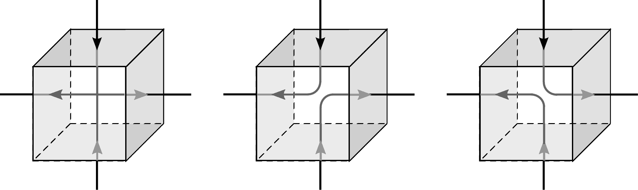
We now consider the length $l$ of vortex loops. As we discussed above, we place straight vortex line elements at the centres of all plaquettes with non-zero flux $|v_{\bm{x}}^{a}|=1$ and we connect them with the constraint of not crossing the lines. The length of each loop is even in units of $\Delta x$ and the minimal length is $4\Delta x$ . When four or more plaquettes in one unit cube have non-zero flux, i.e., four or more vortex elements pierce the cube, we have to decide how to connect the vortex elements. This is shown in Fig. 11. Several criteria to connect vortex elements are discussed in Refs. [28, 29]. We adopt the maximal and stochastic ones. The connection is uniquely done so that the vortex loops are joined as much as possible to form a long vortex loop in the maximal criterion, see Fig. 12, while the connection is done at random with equal probability among all possible ways to connect them in the stochastic criterion. These crossings give rise to vortex recombination. We verified that all vortices take the form of a closed loop as we expect from the topological prospect for vortices.

Figures 13 (a)-(d) show snapshots of equilibrium system configurations where the vortex line elements at the centre of the plaquettes with non-zero flux are highlighted. The temperatures of the different snapshots are $T=0.6\ T_{\mathrm{c}}$ , $T=0.8\ T_{\mathrm{c}}$ , $T=T_{\mathrm{c}}$ , and $T=1.2\ T_{\mathrm{c}}$ , from left to right. Upper and lower panels show the same configurations with the vortex elements connected with the maximal criterion (upper panels) and the stochastic criterion (lower panels). At low temperatures, the way in which the elements are connected is irrelevant as the vortex rings are very short, as shown in Fig. 13 (a). We checked that these vortices are rapidly created by thermal fluctuations as small vortex rings and they are soon annihilated. It should be hard to experimentally observe such vortices due to the fact that their dynamics occur in very short time scales. Accordingly, $\rho_{\mathrm{vortex}}$ is well-fitted by the Arrhenius law $\rho_{\mathrm{vortex}}\propto e^{-\varepsilon/T}$ with the activation energy $\varepsilon\simeq 6.63$ as shown in Fig. 10 (b).

At higher temperature, the vortex loops are longer and the method used to connect the vortex elements becomes important. The comparison between the upper and lower snapshots in Fig. 13 (b)-(d) demonstrate that the longest vortex loop is much longer with the maximal than with the stochastic connection rule.

The fact that the vortex loops are longer at higher temperature can also be seen from Fig. 14. Panels (a) and (c) show the number of vortex loops with length $l$ , $N^{\mathrm{(M)}}(l)$ calculated with the maximal criterion (upper panel) and $N^{\mathrm{(S)}}(l)$ with the stochastic criterion (lower panel) for connecting vortex lines, at four temperatures around the critical one, $T=0.8\ T_{c},\ T_{c},1.2\ T_{c},2\ T_{\mathrm{c}}$ . At $T=0.8\ T_{\mathrm{c}}$ the number density decays exponentially, see also panel (a) in Fig. 15, irrespectively of the reconnection method used. (This quantity can be turned into a probability distribution with its normalisation by the total number of loops in the system, $\int dl\>N^{\mathrm{(M,S)}}(l)=N^{\mathrm{(M,S)}}_{\mathrm{loop}}$ . As in the dynamic study we will see that this quantity depends on time, we avoid imposing this normalisation.)

As temperature increases from $0.8\ T_{\mathrm{c}}$ , longer loops appear and the size of the longest loop increases, as shown by the fact that the support of $N^{\mathrm{(M,S)}}(l)$ extends further away on the horizontal axis. With the maximal rule, $N^{\mathrm{(M)}}(l)$ gets close to a power-law, $N^{\mathrm{(M)}}(l)\sim l^{-2.17}$ at $T\simeq 0.95\ T_{\mathrm{c}}$ and a sharp peak at very large value of $l$ starts developing at this temperature (see the solid line in panel (b) where data for more values of $T$ approaching $T_{\mathrm{c}}$ from below are shown). This bump suggests the existence of very long vortex rings that could wrap around the system many times, see Fig. 15 (b) where the system size dependence of the bump is shown explicitly (we will address this issue in detail below). At still higher temperature $T>0.95\ T_{\mathrm{c}}$ the weight of the finite size loops decreases but the bump remains and gets thinner as less loops with length of the order of the system size exist but their length fluctuates less. It may become possible to observe such large-scale vortices as a macroscopic fluctuation of the fluid vorticity.

We also stress the difference between $N^{\mathrm{(M)}}(l)$ and $N^{\mathrm{(S)}}(l)$ . At temperatures far below $T_{\mathrm{c}}$ ( $T=0.8\ T_{\mathrm{c}}$ in Fig. 14 (a)), there is basically no difference between the data for the two reconnection rules. However, the statistics of the strings strongly depends on the reconnection rule at temperatures close and above $T_{\mathrm{c}}$ . The power law $l^{-2.17}$ is close to the data for finite loops approaching $T_{\mathrm{c}}$ from below for both reconnection rules (panels (b) and (d)) but the behaviour of the distribution at larger scales are totally different. A bump structure in $N^{\mathrm{(M)}}(l)$ is sharp and clearly seen (panels (a) and (b)), whereas the statistics of long closed strings at high temperature as obtained with the stochastic criterium crosses over between two power-law decays. At $T=2\ T_{\mathrm{c}}$ , for $\Delta x\ll l\ll L^{2}$ the chains are Gaussian and $N^{\mathrm{(S)}}(l)\simeq l^{-5/2}$ while for $l\gg L^{2}$ the fact that the loops can wrap around the cubic box changes this decay and makes it be $N^{\mathrm{(S)}}(l)\simeq l^{-1}$ . These two powers are shown with a dashed and dashed lines in panes (c) and (d) where the second power law regime is just incipient at $T=0.99\ T_{\mathrm{c}}$ . The first power law was also observed in the random phase clock model studied in [84, 85] and it is well-known in the field of polymer science [74]. The cross-over to the second decay was observed and explained in [89] where a fully-packed loop model arising in the ice phase of a frustrated magnetic system on the pyrochlore lattice was studied and, in more general terms, in [90, 30]. Although our system is not fully-packed with loops, the density of vortex elements is very high at high temperature (e.g. $\rho_{\mathrm{vortex}}\simeq 0.25$ at $T=2\ T_{\mathrm{c}}$ ) and the behaviour is quite similar.

The qualitative change of the vortex line length distribution and its dependence on the connecting criteria can already be seen in Figs. 13 (a)-(d) where the longest vortex line is highlighted (in yellow). On the one hand, in panels (a) and (b), at temperatures well below $T_{\mathrm{c}}$ , the longest vortex loop is very short compared to the system size. On the other hand, in panels (c) and (d), at temperatures at and above $T_{\mathrm{c}}$ , respectively, most vortex line elements belong to the longest vortex loop, the spatially dominating scale of which is comparable to the system size. The longest vortex determined by the maximal criterion is much longer than the one obtained with the stochastic criterion. Indeed, the longest vortex loop obtained with the maximal criterion contains almost all vortex line elements, and contributes to the sharp bump in $N^{\mathrm{(M)}}(l)$ at large $l$ . With the stochastic convention, instead, there are many long vortex loops besides the longest one, making $N^{\mathrm{(S)}}(l)$ broader. What is the fraction of vortex mass in an infinite loop is a question of interest in cosmology [85].

We now compare the length number density per unit volume $N^{\mathrm{(M,S)}}(l)/L^{3}$ in systems with different size. Figures 15 shows this quantity at temperatures $T=0.8\ T_{\mathrm{c}}$ (a) and (c), and $T=T_{\mathrm{c}}$ (b) and (d). At $T=0.8\ T_{\mathrm{c}}$ , there is no finite size dependence and there are no long vortices with size comparable to the system size. At $T=T_{\mathrm{c}}$ , on the other hand, the weight of the number density clearly depends on the system size, suggesting the existence of very long vortex loops with lengths comparable and increasing with the system size. With the maximal convention the tail of the number density, before the bump, bends down and, clearly, it is not algebraic. With the stochastic one, the data at $T_{\mathrm{c}}$ suggest a smooth crossover from $l^{-2.17}$ at short length scales to a different behaviour at long length scales; we will discuss this issue in the next paragraph where we will study the percolation phenomenon in detail and we will find that the percolation threshold with the stochastic convention although very close to $T_{\mathrm{c}}$ is not at $T_{\mathrm{c}}$ .

IV.5 The randomly reconnected data in the infinite temperature limit

We consider now the infinite temperature data and the string length derived with the stochastic criterium in more detail and we compare it to predictions for fully-packed loop models of different kind.

It was shown in [89, 90] that the number density of loop lengths in quite generic fully-packed loop models behaves as

\displaystyle\frac{lN(l)}{L^{3}}\simeq\left\{\begin{array}[]{rcl}\displaystyle l^{-d/2}&\qquad\mbox{for}&\qquad\Delta x\ll l\ll L^{2}\\ \displaystyle L^{-3}&\qquad\mbox{for}&\qquad L^{2}\ll l\ll L^{3}\end{array}\right.

as the fractal dimension of the loops at the largest scale is $3$ in our case. (Corrections to the power in the second line should be taken into account for $l\simeq L^{3}$ and these depend on the model [90].) Gaussian statistics for $l\ll L^{2}$ was also found numerically in the nodal statistics of $3d$ complex random wave fields [12, 13].

In Fig. 16 we show $N^{\mathrm{(S)}}(l)$ against $l$ (a) and $N^{\mathrm{(S)}}(l)$ against $l/L^{2}$ (b). Data for different system sizes are gathered in the two panels. We see in (a) that the data do not depend on $L$ for lengths that are shorter than $L^{2}$ while they do for longer scales. In (b) the data for $l\ll L^{2}$ keep the Gaussian statistics (dashed lines) and what remains scales well with the proposed scaling variable. The dotted curve is the expected $l^{-1}$ decay in Eq. (IV.5). The scaling of the second tail data with the fractal dimension $3$ is good, and an analogue between $N^{\mathrm{(S)}}(l)$ in the $T\to\infty$ limit and loop soups is thus confirmed.

IV.6 Vanishing line-tension characteristic temperature

There are several ways to discuss line percolation in this kind of systems and they do not yield the same threshold [28, 29]. For this reason, we will be specially careful here.

We adopted the method based on the number density $N^{\mathrm{(M,S)}}(l)$ . Below and close to its threshold, in the infinite system size limit, $N^{\mathrm{(M,L)}}(l)$ should behave as in Eq. (57)

\displaystyle N^{\mathrm{(M,S)}}(l)\propto l^{-\alpha^{\mathrm{(M,S)}}_{\mathrm{L}}}\ e^{-lm^{\mathrm{(M,S)}}_{\mathrm{L}}}

(73)

with the “Fisher” exponent $\alpha^{\mathrm{(M,S)}}_{\mathrm{L}}=1+d/D^{\mathrm{(M,S)}}_{\mathrm{L}}$ being related to the fractal dimension, $D^{\mathrm{(M,S)}}_{\mathrm{L}}$ , of the vortex lines, and the “mass” $m^{\mathrm{(M,S)}}_{\mathrm{L}}$ that vanishes at the threshold. Following Ref. [28], we call this temperature the line-tension point $T^{\mathrm{(M,S)}}_{\mathrm{L}}$ .

In Fig. 14 (b) we show the length number density $N^{\mathrm{(M)}}(l)$ at $T=0.93\ T_{\mathrm{c}}$ , $0.94\ T_{\mathrm{c}}$ , $0.95\ T_{\mathrm{c}}$ , $0.96\ T_{\mathrm{c}}$ , and $0.97\ T_{\mathrm{c}}$ with the maximal line-reconnection criterion (upper panel), and $N^{\mathrm{(S)}}(l)$ at $T=0.95\ T_{\mathrm{c}}$ , $0.96\ T_{\mathrm{c}}$ , $0.97\ T_{\mathrm{c}}$ , $0.98\ T_{\mathrm{c}}$ , and $0.99\ T_{\mathrm{c}}$ with the stochastic line-reconnection criterion (lower panel) for the largest system size that we simulated, $L=100$ . At $0.94\ T_{\mathrm{c}}$ ( $0.98\ T_{\mathrm{c}}$ ) the data are close to algebraic with an incipient bump at the largest scales in the upper (lower) panel. The short length-scale, say $10^{2}\lesssim l\lesssim 10^{3}$ , behaviour of $N^{\mathrm{(M,S)}}(l)$ is rather well fitted by

\displaystyle N^{\mathrm{(M,S)}}(l)\propto l^{-\alpha^{\mathrm{(M,S)}}_{\mathrm{L}}}\qquad\mbox{with}\qquad\alpha^{\mathrm{(M,S)}}_{\mathrm{L}}\simeq 2.17\;.

(74)

Figure 17 (a) shows the mass $m^{\mathrm{(M,S)}}_{\mathrm{L}}$ extracted from fits with the full function (73) with the exponent $\alpha^{\mathrm{(M,S)}}_{\mathrm{L}}$ fixed to $\alpha^{\mathrm{(M,S)}}_{\mathrm{L}}=2.17$ . From the data fits the mass $m^{\mathrm{(M)}}_{\mathrm{L}}$ ( $m^{\mathrm{(S)}}_{\mathrm{L}}$ ) vanishes at $T\simeq 2.13\simeq 0.94\ T_{\mathrm{c}}$ ( $T\simeq 2.22\simeq 0.98\ T_{\mathrm{c}}$ ). We therefore estimate the temperature at which $N^{\mathrm{(M,S)}}(l)$ is purely algebraic as

\displaystyle\begin{split}T^{\mathrm{(M)}}_{\mathrm{L}}\simeq 2.13\simeq 0.94\ T_{\mathrm{c}},\qquad T^{\mathrm{(S)}}_{\mathrm{L}}\simeq 2.22\simeq 0.98\ T_{\mathrm{c}},\end{split}

(75)

and they do not coincide with the one for the thermodynamic instability $T_{\mathrm{c}}$ , see the analysis in Sec. III. In the temperature range $0.05\leq T^{\mathrm{(M,S)}}_{\mathrm{L}}-T\leq 0.1$ , the masses $m^{\mathrm{(M,S)}}_{\mathrm{L}}$ for the system sizes $L=80$ and $L=100$ are rather well fitted by

m^{\mathrm{(M,S)}}_{\mathrm{L}}\propto(T^{\mathrm{(M,S)}}_{\mathrm{L}}-T)^{\beta^{\mathrm{(M,S)}}_{\mathrm{L}}}\qquad\mbox{with}\qquad\beta^{\mathrm{(M,S)}}_{\mathrm{L}}\simeq 1.7\;.

(76)

This value hardly depends on the criteria for connecting vortices and is consistent with the results obtained with Monte Carlo simulations of the $3d$ $XY$ -model [28] and this model [29]. Figure 17 (b) shows the length number density per unit volume $N^{\mathrm{(M,S)}}(l)/L^{3}$ for systems with different linear sizes at the vortex line-tension point $T^{\mathrm{(M,S)}}_{\mathrm{L}}$ . Except for the bump structure in the region of long $l$ , $N^{\mathrm{(M,S)}}(l)/L^{3}$ at $T=T^{\mathrm{(M,S)}}_{\mathrm{L}}$ does not depend upon $L$ .

Finally, we note that simulations with different $\Delta x$ give different values for $T_{\mathrm{c}}$ , $T_{\mathrm{L}}^{\mathrm{(M)}}$ , and $T_{\mathrm{L}}^{\mathrm{(S)}}$ , but the algebraic behaviour at the vortex line-tension point hardly depends on $\Delta x$ with the same exponents $\alpha_{\mathrm{L}}^{\mathrm{(M,S)}}\simeq 2.17$ and $\beta_{\mathrm{L}}^{\mathrm{(M,S)}}\simeq 1.7$ within our numerical accuracy.

IV.7 The bump

We consider now the bump structure in the number density $N^{\mathrm{(M,S)}}(l)$ . A bump in the number density $N^{\mathrm{(M,S)}}(l)$ at large value of $l$ starts to develop at $T^{\mathrm{(M,S)}}_{\mathrm{L}}$ and is due to the finite size of the system. To describe it one should write a finite system size additive correction [81] to the vortex length distribution $N^{\mathrm{(M,S)}}(l)$ in (73):

\displaystyle N^{\mathrm{(M,S)}}_{\mathrm{finite\ size\ corr}}(l)=N^{\mathrm{(M,S)}}_{\mathrm{L}}\big(\tilde{l}^{\mathrm{(M,S)}}\big),\qquad\tilde{l}^{\mathrm{(M,S)}}\equiv l/L^{D^{\mathrm{(M,S)}}_{\mathrm{L}}}

(77)

with $N^{\mathrm{(M,S)}}_{\mathrm{L}}\big(0\big)=0$ . Equation (77) states that the finite size correction to the number density $N^{\mathrm{(M,S)}}(l)$ should be a universal function of $\tilde{l}^{\mathrm{(M,S)}}\equiv l/L^{D^{\mathrm{(M,S)}}_{\mathrm{L}}}$ with $D^{\mathrm{(M,S)}}_{\mathrm{L}}=d/(\alpha^{\mathrm{(M,S)}}_{\mathrm{L}}-1)\simeq 2.56$ the fractal dimension of the lines and $d=3$ the dimension of space.

Figures 18 (a) and (b) show $\big(l^{\mathrm{(M,S)}}\big)^{\alpha_{\mathrm{L}}^{\mathrm{(M,S)}}}\>N^{\mathrm{(M,S)}}(l)$ as a function of $\tilde{l}^{\mathrm{(M,S)}}$ , at $T^{\mathrm{(M,S)}}_{\mathrm{L}}$ and $T_{\mathrm{c}}$ , respectively, and for the system sizes $L=40$ , $60$ , $80$ , $100$ . After multiplying by $\big(l^{\mathrm{(M,S)}}\big)^{\alpha_{\mathrm{L}}^{\mathrm{(M,S)}}}$ the finite length contribution should become just an irrelevant additive constant and all the variation is due to the finite system-size correction. The universal behaviour of the bump structure as shown in Eq. (77) holds at $T^{\mathrm{(M,S)}}_{\mathrm{L}}$ and it does not at $T_{\mathrm{c}}$ , confirming the fact that line percolation occurs at $T_{\mathrm{L}}^{\mathrm{(M,S)}}$ .

IV.8 Mean number of vortex loops

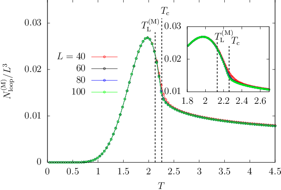
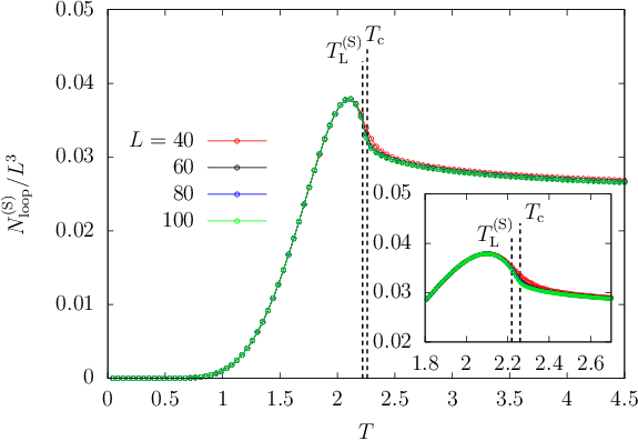
Figure 19 shows the temperature dependence of the mean number of vortex loops

N^{\mathrm{(M,S)}}_{\mathrm{loop}}\equiv\langle\text{total number of vortex loops}\rangle_{\mathrm{stat}}

(78)

normalized by the size of the simulation box $L^{3}$ . $N^{\mathrm{(M)}}_{\mathrm{loop}}$ is consistently smaller than $N^{\mathrm{(S)}}_{\mathrm{loop}}$ . Both figures show no $L$ dependence. At low temperatures, $N^{\mathrm{(M,S)}}_{\mathrm{loop}}$ is an increasing function of temperature. Above a temperature that is slightly lower than $T_{\mathrm{L}}^{\mathrm{(M,S)}}$ , $N^{\mathrm{(M,S)}}_{\mathrm{loop}}$ reaches a maximum and next decreases with increasing temperature, suggesting that many small vortex rings merge to form longer loops, as $\rho_{\mathrm{vortex}}$ is still increasing with temperature. The fact that $N^{\mathrm{(M)}}_{\mathrm{loop}}$ decreases faster than $N^{\mathrm{(S)}}_{\mathrm{loop}}$ with temperature is due to the fact that more vortex elements are joined to the longest vortex loop with the maximal than with the stochastic rule. Notably, the curvature of the curves changes at $T_{\mathrm{c}}$ but we do not see any special feature at $T_{\mathrm{L}}^{\mathrm{(M,S)}}$ .

IV.9 Wrapping vs. contractible loops

As discussed above, the scaling of the bump in $N^{\mathrm{(M,S)}}(l)$ , and the peak and tail in $N^{\mathrm{(M)}}(l)$ and $N^{\mathrm{(S)}}(l)$ at high temperature, suggest the existence of very long vortex loops with length of the order of, or even much longer than, $L$ . In order to distinguish loops that wrap around the system from long but contractible loops, we define and calculate two quantities.

The first observable just focuses on the size of the vortices, that we define as the maximal side of the rectangular parallelepiped covering the vortex loop in the $x$ , $y$ , and $z$ -directions (see Fig. 20). The size is the length the string would have after smoothing out all small scale irregularities (and it yields a length scale similar to $R$ in Eq. (56)).

We then count the number of vortex loops, the size of which is larger than the system size $L$ , and we calculate the statistical average:

\displaystyle\begin{split}&N^{\mathrm{(M,S)}}_{\mathrm{system-size}}\equiv\langle\text{Number of vortex loops, the size of which is larger than $L$}\rangle_{\mathrm{stat}}.\end{split}

(79)

Figure 21 (a) shows the temperature dependence of the fraction $N^{\mathrm{(M)}}_{\mathrm{system-size}}/N^{\mathrm{(M)}}_{\mathrm{loop}}$ . It detaches from zero at $T\simeq 0.59\simeq 0.26\ T_{\mathrm{c}}$ (while $\rho_{\mathrm{vortex}}$ detaches from zero at $T\simeq 0.32\simeq 0.14\ T_{\mathrm{c}}$ ) and has a peak at a temperature that is very close to the value of $T_{\mathrm{L}}^{\mathrm{(M)}}$ found with the analysis of $N^{\mathrm{(M)}}(l)$ in the infinite system size limit.

The behaviour of $N_{\mathrm{system-size}}^{\mathrm{(S)}}$ shown in Fig. 21 (c) is quantitatively different from the one of $N_{\mathrm{system-size}}^{\mathrm{(M)}}$ : it does not have a peak and it detaches from zero at a temperature slightly lower than $T^{\mathrm{(S)}}_{\mathrm{L}}$ found with the analysis of $N^{\mathrm{(M)}}(l)$ . At a temperature very close to $T^{\mathrm{(S)}}_{\mathrm{L}}$ , $N_{\mathrm{system-size}}^{\mathrm{(S)}}$ loses its size dependence and $N_{\mathrm{system-size}}^{\mathrm{(S)}}\simeq 1.07$ . In the limit of infinite system size $L\to\infty$ , one may expect a sharp transition from $N_{\mathrm{system-size}}^{\mathrm{(S)}}=0$ to $N_{\mathrm{system-size}}^{\mathrm{(S)}}>1$ at $T^{\mathrm{(S)}}_{\mathrm{L}}$ .

With the second method we count only non-contractible loops that are topologically distinct from contractible ones due to the periodic boundary condition. We can check whether a vortex loop is non-contractible or not in the following way. We set the winding numbers along the $x$ , $y$ , and $z$ -directions to zero, $w_{x}=w_{y}=w_{z}=0$ . We then start from a point on the loop and we follow the loop path. When the loop jumps from $(0,y,z)$ ( $(L,y,z)$ ) to $(L,y,z)$ $((0,y,z))$ , we change $w_{x}\to w_{x}+1$ ( $w_{x}\to w_{x}-1$ ). In the same manner we update $w_{y}$ and $w_{z}$ when going across the system’s “boundary” in the $y$ and $z$ directions. After going back to the starting point, at least one of the three winding numbers $w_{x}$ , $w_{y}$ , and $w_{z}$ take non-zero value when the loop is non-contractible.

We define $N_{\mathrm{non-contract}}$ as

\displaystyle\begin{split}&N_{\mathrm{non-contract}}\equiv\langle\text{Number of non-contractible vortex loops}\rangle_{\mathrm{stat}}.\end{split}

(80)

We should note that the summation of winding numbers for all vortex loops vanishes identically:

\displaystyle\sum_{\mathrm{loops}}(w_{x},w_{y},w_{z})=(0,0,0)

(81)

showing that there is no net rotational flow. Another property is that $N^{\mathrm{(M,S)}}_{\mathrm{system-size}}\geq N^{\mathrm{(M,S)}}_{\mathrm{non-contract}}$ . Figure 22 shows examples of contractible and non-contractible vortex loops. In Fig. 22 (a), there is one long contractible vortex loop, the size of which is larger than the system linear size. Through the reconnection of two vortex elements in the loop, the contractible vortex loop splits into two non-contractible vortex loops as shown in the panel (b) in the same figure.

Figure 23 (a)-(c) shows the longest vortex loops in three equilibrium configurations at $T=T^{\mathrm{(S)}}_{\mathrm{L}}$ . The vortex elements were connected using the stochastic criterion. In panel (a), the size the vortex loop is smaller than the system size $L$ . Although the sizes of vortex loops are larger than the system size in panels (b) and (c), the vortex loop in panel (b) is contractible while the one in panel (c) is non-contractible in the vertical direction.

Figure 21 (b) shows the temperature dependence of $N^{\mathrm{(M)}}_{\mathrm{non-contract}}$ (upper panel) and $N^{\mathrm{(S)}}_{\mathrm{non-contract}}$ (lower panel). With the maximal criterium for connecting vortex elements, we have $N^{\mathrm{(M)}}_{\mathrm{non-contract}}=0$ and there are no non-contractible vortex loops. This a priori surprising results is due to the fact that with the maximal criterium all non-contractible vortex loops get connected to neighboring ones to form a large contractible vortex loop (see Fig. 22: the configuration in panel (a) is preferred because the length of the single vortex loop is longer than the one of the two non-contractible vortices in panel (b)). With the stochastic criterium for connecting vortex elements, we have a finite number of non-contractible vortex loops $N^{\mathrm{(S)}}_{\mathrm{non-contract}}>0$ . As well as $N^{\mathrm{(S)}}_{\mathrm{system-size}}$ in (c), $N^{\mathrm{(S)}}_{\mathrm{non-contract}}$ in (d) loses its size dependence at $T^{\mathrm{(S)}}_{\mathrm{L}}$ (within our numerical accuracy) and $N^{\mathrm{(S)}}_{\mathrm{non-contract}}\simeq 0.532$ . In the limit of infinite system size $L\to\infty$ , we expect a sharp transition from $N_{\mathrm{non-contract}}=0$ to $N_{\mathrm{non-contract}}>0$ at a temperature close to $T^{\mathrm{(S)}}_{\mathrm{L}}$ , which suggests that one vortex loop larger than the system size $L$ at $T=T^{\mathrm{(S)}}_{\mathrm{L}}$ is non-contractible with a probability close to $0.532$ .

From the fact that the number of vortex loops larger than the system size $N^{\mathrm{(S)}}_{\mathrm{system-size}}$ and the number of non-contractible loops $N^{\mathrm{(S)}}_{\mathrm{non-contract}}$ obtained with the stochastic criterium (see Figs. 21 (c) and (d)) are size independent at the vortex line-tension point $T=T_{\mathrm{L}}^{\mathrm{(S)}}$ , we can expect them to be universal functions of $(T_{\mathrm{L}}^{\mathrm{(S)}}-T)/L^{-\nu_{\mathrm{L}}}$ ( $(T-T_{\mathrm{L}}^{\mathrm{(S)}})/L^{-\nu^{\prime}_{\mathrm{L}}}$ ) with some exponents $\nu_{\mathrm{L}}$ ( $\nu_{\mathrm{L}}^{\prime}$ ) at temperatures $T<T_{\mathrm{L}}^{\mathrm{(S)}}$ ( $T>T_{\mathrm{L}}^{\mathrm{(S)}}$ ). Figures 24 (a) ((b)) and (c) ((d)) show $N^{\mathrm{(S)}}_{\mathrm{system-size}}$ and $N^{\mathrm{(S)}}_{\mathrm{non-contract}}$ as functions of $(T_{\mathrm{L}}^{\mathrm{(S)}}-T)/L^{-\nu_{\mathrm{L}}}$ ( $(T-T_{\mathrm{L}}^{\mathrm{(S)}})/L^{-\nu^{\prime}_{\mathrm{L}}}$ ) with $\nu_{\mathrm{L}}=0.76$ ( $\nu_{\mathrm{L}}^{\prime}=0.34$ ). The data show good collapse on both sides of the line-tension point $T_{\mathrm{L}}$ . In Fig. 25 we show the finite size scaling behaviour of $m^{\mathrm{(S)}}_{\mathrm{L}}$ using two exponents $\nu_{\mathrm{L}}$ and $\beta^{\mathrm{(S)}}_{\mathrm{L}}$ for the mass parameter $m^{\mathrm{(S)}}_{\mathrm{L}}$ (see the inset in Fig. 17 (a)).

IV.10 Discussion

In this Section we analysed the statistical properties of the vortex tangle in equilibrium.

The full vortex configuration is independent of the reconnection method and boundary conditions in the low temperature regime. The distribution of vortex lengths is simply exponential.

Different percolation thresholds can be identified by working with different vortex-related observables [28, 29]. A natural characterisation of the loop ensemble is given by their length distribution, from which a critical point is identified as the temperature at which the mass parameter vanishes, the so-called line-tension point. The result $T^{\mathrm{(M,S)}}_{\mathrm{L}}<T_{\mathrm{c}}$ shows that the spontaneous breaking of the U(1) symmetry is not directly connected to the percolation of vortex lines, which is consistent with previous work for the $3d$ XY model [28] and the O(2) model [29], and contrary to claims in [75, 76, 77, 78, 79]. The fact that $T_{\mathrm{L}}^{\mathrm{(M)}}<T_{\mathrm{L}}^{\mathrm{(S)}}$ is reasonable since strings are longer in the former than in the latter case. The critical properties of finite loops remain independent of the reconnection rule and the size of the mesh used to discretize space (within numerical accuracy).

At $T^{\mathrm{(M,S)}}_{\mathrm{L}}$ we find the Fisher exponent $\alpha^{\mathrm{(M,S)}}_{\mathrm{L}}\simeq 2.17$ , and from this value we deduce $D^{\mathrm{(M,S)}}_{\mathrm{L}}\sim 2.56$ . Moreover, $\alpha^{\mathrm{(M,S)}}_{\mathrm{L}}<2.5$ suggests that vortices at the line tension point behave as a self-seeking random walk. Bittner et al [29] found $\alpha_{\mathrm{L}}\simeq 2.26-2.27$ in the continuous O(2) field theory and Kajantie et al [28] $\alpha_{\mathrm{L}}\simeq 2.11$ in Monte Carlo simulations of the $3d$ XY model, both with the stochastic reconnection rule and at the percolation point. Similarly, Ortuño et al. computed $\alpha^{\mathrm{(M,S)}}_{\mathrm{L}}=2.184(3)$ at the critical point of a network model for the disorder-induced localisation transition. We recall that [28] also showed that the percolation-observable critical properties may also depend upon the reconnection rule adopted.

We do not see any special feature in the density of vortex elements or the mean number of vortex lines at the line tension point. However, signatures of the vanishing line tension point are seen in other quantities. We see a maximum in the ratio between the number of loops that are longer than the system size and the total number of loops when the maximal criterium is used (though the height of the maximum decreases with $L$ increasing and we cannot exclude that this effect disappears in the thermodynamic limit). (This feature is not shared by the numerator in this ratio.) The number of vortex loops that are longer than the system size and that are non-contractible constructed with the stochastic criterium behave similarly to an order parameter for the geometric transition. No quantity of this kind for the maximal rule behaves as an order parameter. Interestingly enough, the thermodynamic threshold $T_{\mathrm{c}}$ seems to appear as the temperature at which $\rho_{\mathrm{vortex}}$ and $N_{\mathrm{loop}}^{\mathrm{(M,S)}}$ change concavity.

At high temperature the influence of the reconnection method becomes very important as there are loops with length of the order of the linear size of the system or longer. The boundary conditions also become important. As in the quench dynamic analysis we will use the equilibrium state at high temperature as the initial configuration, it is specially important to characterise the vortex tangle at very high temperature. With the maximal criterium we found that one line carries most of the vortex mass in the sample at very high temperature. With the stochastic criterium we found that the statistics of loops with length $l\ll L^{2}$ is Gaussian while even longer loops exist and their number density falls-off as $(l/L^{3})^{-1}$ .

Vachaspati & Vilenkin [84] used a simple $Z_{3}-symmetric$ model to generate the putative initial conditions of the field theory that should describe the state of the universe before undergoing a phase transition. This is a clock model with three phase values attributed at random with equal probability on each vertex of a regular cubic lattice with open boundary conditions. They used the stochastic rule to reconnect the vortex elements on a cell. Strobl & Hindmarsch increase the number of discrete angles from 3 to 255 in a formally infinite lattice [85]. They both found the statistics of a Gaussian random walk ( $D=2$ ) as for a dense polymer network [74]. At very high temperature the statistics of our loop ensemble, when treated with the stochastic reconnection rule, and for length scales such that $l\ll L^{2}$ , also approaches this result. Instead, the statistics is very different with the maximal reconnection criterium or beyond the crossover at $L^{2}$ .

We note that the behaviour of vortex loops in the three-dimensional model is quite different from the one of the topological defects in the Kosterlitz-Thouless transition of the two-dimensional system. In the latter, the phase transition occurs at the same temperature at which the vortex pairs unbind. In the former, percolation occurs at a different temperature from $T_{\mathrm{c}}$ . This is similar to what happens in the Ising model of magnetism: in two-dimensions the percolation of geometric clusters occurs at the critical temperature while in three-dimensions this is not the case. The fact that percolation of geometric objects does not always occur at the thermodynamic critical phenomenon has been known since the work in [69].

V Fast quench dynamics

In this section, we consider the stochastic dynamics following an instantaneous quench from equilibrium at $T=2\ T_{\mathrm{c}}$ to $T=0$ . The analysis in the previous section allowed us to characterise the vortex configurations at the initial state at high temperature in full detail. Here we will be particularly concerned with the evolution of these states after an infinitely fast deep quench. We will show that during the low temperature dynamics vortex lengths with statistics and fractal dimension numerically identical to the one at the percolation threshold $T_{\mathrm{L}}^{\mathrm{(M,S)}}$ will be relevant, although the quench protocol does not spend any time at nor even close to it. These features exist for all microscopic dynamic rules.

V.1 The initial state

Whether the initial state has an order parameter $\overline{\psi}$ that vanishes or not, can have a highly non-trivial influence on the subsequent dynamics. This fact was derived by Toyoki and Honda [35] and later confirmed numerically [38, 39]. Here, we use equilibrium initial states such that the vortex configuration, see Fig. 26 (a), is characterised by the density $\rho_{\mathrm{vortex}}\simeq 0.25$ in Fig. 10 and the distribution of vortex loop lengths shown in Fig. 14 (a). At $T=2\ T_{\mathrm{c}}$ , the order parameter suffers from finite size corrections and we measure $\overline{\psi}\simeq 0.030$ for $L=20$ , $\overline{\psi}\simeq 0.016$ for $L=30$ , $\overline{\psi}\simeq 0.010$ for $L=40$ , and $\overline{\psi}\simeq 0.0073$ for $L=50$ . These values are small enough for the dynamics to be regarded as subsequent to a zero average field initial condition, i.e., $\overline{\psi}\sim 0$ . This is also confirmed by the fact that the scaling regime is reached independently of the system size $L$ , see Figs. 27 (a)-(d) and Figs. 28 (a)-(d). (In some references, e.g. [39], such quenches are named “critical”. In the statistical physics context a “critical quench” is a quench to the critical temperature $T_{\mathrm{c}}$ , so we rather not use this terminology here.)

The statistical and geometrical properties of the vortex loops at high temperatures were characterised in detail in Sec. IV and we will use this information here.

V.2 The initial stage of evolution

V.2.1 Instability

Let us consider the dynamics in the initial stage of evolution within the mean-field framework. By approximating the initial high temperature state as $\psi(t=0)\simeq 0$ and the time-dependent field as $\psi=\delta\psi=ue^{i(\bm{k}\cdot\bm{x}-\omega t)}+v^{\ast}e^{-i(\bm{k}\cdot\bm{x}-\omega^{\ast}t)}$ , the Bogoliubov-de Gennes equation becomes

\displaystyle\begin{split}\{\omega^{2}/c^{2}-k^{2}+(2\mu+i\gamma_{\mathrm{L}})\omega+g\rho\}u+O(\delta\psi^{2})&=0,\\ \{\omega^{2}/c^{2}-k^{2}-(2\mu-i\gamma_{\mathrm{L}})\omega+g\rho\}v+O(\delta\psi^{2})&=0.\end{split}

(82)

The solution to the linear set of equations is

\displaystyle\begin{split}&\omega_{1}^{\pm}(k)=\frac{-ic^{2}(\gamma_{\mathrm{L}}-2i\mu)\pm c\sqrt{4k^{2}-c^{2}(\gamma_{\mathrm{L}}-2i\mu)^{2}-4g\rho}}{2},\\ &\omega_{2}^{\pm}(k)=\frac{-ic^{2}(\gamma_{\mathrm{L}}+2i\mu)\pm c\sqrt{4k^{2}-c^{2}(\gamma_{\mathrm{L}}+2i\mu)^{2}-4g\rho}}{2}.\end{split}

(83)

$\omega_{1,2}^{-}(k)$ are rapidly decaying modes for all $k$ and vanish in the non-relativistic limit $c\to\infty$ , while $\omega_{1,2}^{+}(k)$ are slowly growing modes for $k\lesssim\sqrt{g\rho}$ and decaying modes for $k\gtrsim\sqrt{g\rho}$ . In the first stage of the ordering process, $\omega_{1,2}^{+}(k\lesssim\sqrt{g\rho})$ are the most important modes. The time scale of the growth is $t_{0}\sim(\mathrm{Im}[\omega_{1,2}^{+}(k)])^{-1}\sim(g\rho-k^{2})^{-1/2}$ and the mean-field approximation breaks down beyond it.

V.2.2 Irrelevance of the reconnection rule

Figure 26 shows the vortex loop configurations at four instants soon after the quench. One sees from the pictures that the reconnection rule used to build the vortex loops becomes irrelevant relatively soon, as the configurations in the upper and lower panels in the column (c) are very similar and in (d) are identical.

V.3 The dynamic correlation length

After a transient, the system is expected to enter a dynamic scaling regime [31] characterised by a growing length scale, $\xi_{\mathrm{d}}(t)\simeq t^{1/z_{\mathrm{d}}}$ . How soon or not this is achieve will be discussed in the following subsections; for the moment we assume the scaling regime established and we study global correlation functions and observables within its framework.

The dynamic exponent in the low temperature phase, $z_{\mathrm{d}}$ , is different from the one found in quenches to the critical point that, in turn, coincides with the equilibrium critical one $z_{\mathrm{eq}}$ discussed in Sec. III.4. We will now determine $z_{\mathrm{d}}$ .

The dynamic growing length, $\xi_{\mathrm{d}}(t)$ , can be measured in different ways by exploiting the dynamic scaling hypothesis [31]. Under this assumption, in the infinite size limit, the space-time correlation function and the dynamic structure factor after a quench to very low-temperatures should scale as

S(k,t)\simeq\xi_{\mathrm{d}}^{d}(t)\ \Phi(k\xi_{\mathrm{d}}(t))\qquad\qquad C(r,t)\simeq f\left(\frac{r}{\xi_{\mathrm{d}}(t)}\right)\;.

(84)

with $\Phi$ and $f$ two scaling functions.

Figures 27 (a)-(d) show the dynamical correlation length $\xi_{\mathrm{d}}$ obtained from

\displaystyle\frac{S(k=2\pi/\xi_{\mathrm{d}}(t))}{S(k\to 0)}=10^{-1},\quad S(k\to 0)\equiv 2S(\Delta k)-S(2\Delta k),

(85)

a similar definition to the one used for the equilibrium correlation length $\xi_{\mathrm{eq}}$ in Eqs. (42). In the algebraic regime, $\xi_{\mathrm{d}}(t)\simeq t^{1/z_{\mathrm{d}}}$ , the estimated exponents, $z_{\mathrm{d}}$ , are 0.43 for the over-damped Langevin equation (11), 0.50 for the under-damped Langevin equation (16), 0.50 for the ultra-relativistic limit of the under-damped Langevin equation (17a), and 0.50 for the non-relativistic limit of the under-damped Langevin equation (17b). We have not observed an appreciable change in the value of $z_{\mathrm{d}}$ by varying the increments in space and time $\Delta x$ and $\Delta t$ in our algorithm for the over-damped evolution.

As we will show in Sec. V.4, the exponents characterising the vortex density $\rho_{\mathrm{vortex}}$ decay, and the growth of the dynamical correlation length $\xi_{\mathrm{d}}$ , are well related by $\xi_{\mathrm{d}}\propto 1/\sqrt{\rho_{\mathrm{vortex}}}$ within numerical accuracy. Again, we obtain a weak discrepancy between our result for the over-damped Langevin equation and the prediction; $\xi_{\mathrm{d}}\propto t^{1/2}$ [36], and good agreement for the other three under-damped Langevin equations. The slight disagreement with theory in the numerical data for the over-damped dynamics was also observed in [38, 39]. We will give a possible reason for it in Sec. V.4.

At sufficient long times and for finite system sizes the growing length saturates. Saturation is observed in the curves for $L\leq 100$ when the curves depart from the power law and reach a plateau. For $L=500$ the saturation is pushed beyond the numerical time window. We postpone the finite-size scaling analysis of the dynamic correlation length in Sec. V.5.

V.4 Time-dependent vortex density

We now examine the phase ordering process from the point of view of the vortex dynamics. In Figs. 26 (a)-(d), we show snapshots of the vortex elements in the initial stage of evolution; $0\leq t\leq 5$ . The two rows compare the loop configurations for the two reconnection conventions for the same field configurations. We have already noted that while the loop configurations are different at very short times, $t=2,\ 3$ , they are the same at the two latest times, $t=4,\ 5$ . In both cases, the longest vortex present in the initial configuration breaks up generating shorter vortex loops, the shortest vortex rings on the scale of the grid are rapidly annihilated, and loops of finite but long length are still present during the evolution.

Our next task is to examine how do the vortex dynamics depend on the evolution equation. Figures 28 (a)-(d) show the $t$ -dependence of the averaged vortex density $\rho_{\mathrm{vortex}}$ as obtained from the Langevin equations (11), (16), (17a), and (17b), respectively. We calculate $\rho_{\mathrm{vortex}}(t)$ from Eq. (69) by replacing the ensemble average $\langle\cdots\rangle_{\mathrm{stat}}$ by an average over 1000 independent initial states in equilibrium at $T=2\ T_{\mathrm{c}}$ .

In the initial stage of evolution for $0\lesssim t\lesssim 5$ , inertial effects are apparent in the behaviour of $\rho_{\mathrm{vortex}}(t)$ for the under-damped dynamics and the ultra-relativistic limit independently of the system size, as shown in Figs. 28 (b) and (c). These are absent in Figs. 28 (a) and (d) with $c\to\infty$ .

After a short transient of the order of $t\simeq 5$ for our system sizes, the vortex density enters the proper scaling regime in which $\rho_{\mathrm{vortex}}(t)$ should be proportional to $t^{-1}$ [31, 36]. The numerical exponents are, however, weakly dependent on the type of Langevin equation; we measure $-0.86$ for the over-damped Langevin equation (11) (a) (for comparison, the algebraic decay $t^{-1}$ is also shown in this figure), $-1.0$ for the under-damped Langevin equation (16) (b), $-1.0$ for the ultra-relativistic limit of the under-damped Langevin equation (17a) (c), and also $-1.0$ for the non-relativistic limit of the under-damped Langevin equation (17b) (d). The value $-0.86$ for the over-damped Langevin equation is similar the value $-0.90(2)$ found in [38, 39] using a cell-dynamics integration scheme. On the other hand, the under-damped Langevin equation and its ultra-relativistic and non-relativistic limits give values that are much closer to the analytic ones.

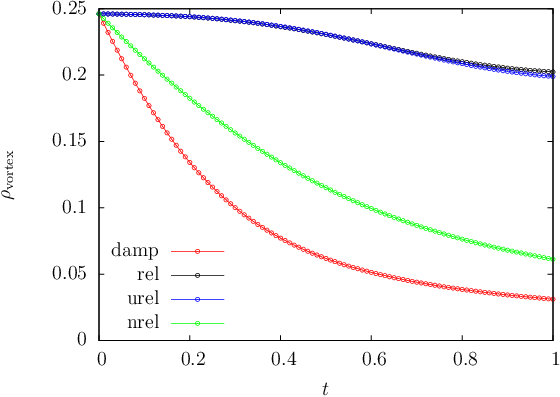
We have calculated the dynamic correlation length and the vortex density using other values of the time and space discretisation parameters and we found essentially the same estimates for the exponent $z_{\mathrm{d}}$ with deviation from the expected value $z_{\mathrm{d}}=2$ for the over-damped dynamics. We may ascribe the origin of this difference to the fact that with this kind of dynamics the vortices are very soon diluted in the sample, for times $0\leq t\lesssim 1$ see Fig. 30, and they cannot properly reach their own scaling regime.

The various curves in each panel in Fig. 29 correspond to different linear system sizes given in the keys. The time lapse over which the dynamics remain in the dynamic scaling regime is no more than a decade for $L\leq 100$ and finite size effects are causing the departure of these curves from a master one and their rapid bending down. This effect is pushed beyond the maximal time simulated for the largest system size, $L=500$ .

The two complementary panels in Fig. 30 make manifest the differences induced by the dynamic equations in the initial instants. The short-time evolution of $\rho_{\mathrm{vortex}}$ and $\xi_{\mathrm{d}}$ are the fastest for the over-damped dynamics (11), intermediate for the non-relativistic limit of the under-damped equation (17b) and the slowest for under-damped (16) and ultra-relativistic limit of this same equation (17a) that yield undistinguishable curves on these plots.

Figures 29 (a)-(d) display snapshots of the vortex elements in a system with linear size $L=60$ at times $t=5,\ 10,\ 15,\ 20$ , in the early stages of the dynamic scaling regime. In all panels the longest vortex loop is highlighted. The percolation across the system of these vortices is confirmed by counting the number of vortex loops the size of which is larger than the system size $N_{\mathrm{system-size}}^{\mathrm{(M,S)}}$ and the number of non-contractible loops $N_{\mathrm{non-contract}}^{\mathrm{(M,S)}}$ . Figures 31 (a)-(d) show $N_{\mathrm{system-size}}^{\mathrm{(M,S)}}$ and $N_{\mathrm{non-contract}}^{\mathrm{(M,S)}}$ in a system with linear size $L=100$ . The power-law behaviour is apparent at $7\lesssim t\lesssim 85$ for the over-damped dynamics (panel (a)), $9\lesssim t\lesssim 90$ for the under-damped dynamics (panel (b)), $8\lesssim t\lesssim 95$ for the ultra-relativistic limit of the under-damped dynamics (panel (c)), and $9\lesssim t\lesssim 150$ for the non-relativistic limit of the under-damped dynamics (panel (d)). In these power-law regimes, there is little difference between the results for the maximal and stochastic criteria for connecting vortex-line elements. We also see that 1 or 2 vortices contribute to $N_{\mathrm{system-size}}^{\mathrm{(M,S)}}$ and $N_{\mathrm{non-contract}}^{\mathrm{(M,S)}}$ .

Figures 32 (a)-(d) show snapshots of the vortex elements in a system with linear size $L=100$ at four later times in the interval $50\leq t\leq 200$ , that is to say, in the late stages of the dynamic scaling regime and the final approach to equilibrium. At $t=50$ , panel (a), $\rho_{\mathrm{vortex}}(t)$ enters the power-law $t^{-1}$ regime. At $t=100$ , panel (b), the dynamics exit this scaling regime. In panels (a) and (b) the size of the longest vortex loop is larger than the system size. At $t=150$ and $200$ (panels (c) and (d)), $\rho_{\mathrm{vortex}}(t)$ decays faster than $t^{-1}$ , and there are only finite size contractible vortices left, which just shrink via the viscosity.

V.5 Finite-size scaling of $\xi_{\mathrm{d}}$ and $\rho_{\mathrm{vortex}}$

Here, we discuss the finite-size scaling properties of the vortex density $\rho_{\mathrm{vortex}}(t)$ and the dynamic correlation length $\xi_{\mathrm{d}}(t)$ .

Since the dynamic correlation length grows in time as $\xi_{\mathrm{d}}(t)\propto t^{1/z_{\mathrm{d}}}$ in the infinite system size limit, $\rho_{\mathrm{vortex}}(t)$ and $\xi_{\mathrm{d}}(t)$ are expected to be universal functions of $t/L^{\mathrm{z_{\mathrm{d}}}}$ in the late stages of evolution of finite size systems:

\frac{\xi_{\mathrm{d}}}{L}=f_{\xi}\left(\frac{t}{L^{z_{\mathrm{d}}}}\right)\qquad\mbox{and}\qquad\rho_{\mathrm{vortex}}=f_{\rho}\left(\frac{t}{L^{z_{\mathrm{d}}}}\right)\;.

(86)

Figures 33 (a) and (b) show $\rho_{\mathrm{vortex}}(t)$ and $\xi_{\mathrm{d}}(t)$ as functions of $t/L^{\mathrm{z_{\mathrm{d}}}}$ with $z_{\mathrm{d}}=2$ obtained from the under-damped Langevin equation at $T=0$ . Except for the initial stage of evolution where another scaling variable characterising the approach to a percolating structure may also be necessary [50], the universal behaviour is good.

We note that similar good universal properties have been obtained using the ultra-relativistic limit of the under-damped Langevin equation (17a), and the non-relativistic limit of the under-damped Langevin equation (17b) at $T=0$ with the same dynamical critical exponent $z_{\mathrm{d}}$ .

With the over-damped Langevin dynamics (11) at $T=0$ , we measured a different dynamical exponent $1/z_{\mathrm{d}}\simeq 0.43$ in Fig 28 (a) for the vortex density and Fig. 27 (a) for the dynamic correlation length. We then compare the scaling with the two dynamical exponents $1/z_{\mathrm{d}}=0.5$ and $0.43$ . Figure 34 shows $\rho_{\mathrm{vortex}}(t)$ (panels (a) and (b)) and $\xi_{\mathrm{d}}(t)$ (panels (c) and (d) as functions of $t/L^{\mathrm{z_{\mathrm{d}}}}$ with $z_{\mathrm{d}}=2$ (panels (a) and (c)) and $1/z_{\mathrm{d}}=0.43$ (panels (b) and (d)) and these dynamics. As expected, in Figs. 28 (a) and 27 (a), we find better universal behaviour with $1/z_{\mathrm{d}}=0.43$ , although the analytic expectation for $1/z_{\mathrm{d}}$ is $0.5$ .

V.6 Number densities of string lengths

We now analyse the statistics of vortex lengths in the course of time. We have already identified three time regimes from the study of the growing length and vortex density: transient, dynamic scaling, and saturation. We therefore study the vortex length statistics in each of these regimes separately.

V.6.1 Short-time transient

We first focus on the short-time transient, say $t\leq 7$ , just before $\rho_{\mathrm{vortex}}$ enters the scaling regime in which the space-time correlation scales with the growing length and the vortex density $\rho_{\mathrm{vortex}}$ relaxes algebraically. As already observed in the analysis of $\rho_{\mathrm{vortex}}$ the reconnection rule and microscopic dynamics affect the observations during this transient. Accordingly, we present the data for the stochastic and maximal criteria separately.

Figure 35 shows the number of vortex loops with length $l$ , i.e. $N^{\mathrm{(M)}}(l,t)$ , in the initial stage of evolution obtained with the maximal criterium for vortex reconnection. We recall that initially $N^{\mathrm{(M)}}(l)$ is given by the (blue) data in Fig. 14 (a) with an exponential decay for finite size loops and a very sharp peak at $l\simeq L^{3}$ .

First, we confirm that the dependence on the microscopic dynamics is very strong during this initial period but it disappears at around $t\simeq 7$ .

Second, we can see that the peak at long $l$ is progressively washed out as the very long loops break up into smaller ones.

Third, we observe that the curves at $t\simeq 7$ have three distinct length regimes with smooth crossovers between them:

- an incipient smooth increase at very short lengths, say $l\lesssim 20$ ,

- an algebraic decay, $\simeq l^{-2.17}$ , at $20\lesssim l\lesssim 200$ and

- a slower algebraic decay, $\simeq l^{-1}$ , at $200\lesssim l$ .

A very interesting feature of these curves is that the algebraic dependence after $l\gtrsim 20$ for $t=3-7$ strongly resembles the power-law decay of the number densities $N^{\mathrm{(M,S)}}(l)$ at the percolation temperature $T_{\mathrm{L}}^{\mathrm{(M,S)}}$ shown in Fig. 17, $N^{\mathrm{(M,S)}}(l,t)\propto l^{-2.17}$ , see the dashed line included as a guide-to-the-eye in all panels. This fact suggests that the early dynamics spontaneously takes the system close to a percolating state similar to the equilibrium one at the percolation threshold $T_{\mathrm{L}}^{\mathrm{(M)}}$ .

Another fact to remark is the disappearance of the peak at very large $l$ (a feature of the initial condition treated with the maximum rule that is absent from the data analysed with the stochastic one) and the generation of the $l^{-1}$ tail characteristic of fully-packed loop models (that was absent initially for this recombination rule).

In order to check the scenario of the spontaneous approach to the percolating state, we study the scaling of the large vortex loop weight as done in Fig. 18 with the same scaling variable $\tilde{l}^{\mathrm{(M)}}=l/L^{D^{\mathrm{(M)}}_{\mathrm{L}}}$ and the fractal dimension $D^{\mathrm{(M)}}_{\mathrm{L}}=d/(\alpha_{\mathrm{L}}^{\mathrm{(M)}}-1)\simeq 2.56$ (see [50] for a similar analysis of the quench dynamics of the $2d$ Ising model). Just after the quench, around $t=1$ , the number density $N^{\mathrm{(M)}}(l,t)$ is not universal with strong size-dependence. As time elapses, the size-dependence gets weaker, and a scaling behaviour at large $l$ establishes at $t\simeq 10$ as shown in panel (d). We can therefore conclude that the system enters the scaling regime around $t\sim 10$ , and that this value does not strongly depend on the exact form of the Langevin equation. We note that the data for linear system size $L=40$ slightly deviates from the scaling behaviour.

Figure 37 shows $N^{\mathrm{(S)}}(l,t)$ calculated with the stochastic criterium for vortex reconnections. We recall that initially, $N^{\mathrm{(S)}}$ is given by the (blue) data in Fig. 14 (c) with a broken algebraic decay with exponents $5/2$ (Gaussian, lengths shorter than $L^{2}$ ) and $1$ (fully-packed, very long). All panels demonstrate the development of three length-scale regimes in the data-sets; again, very short lengths, $l\lesssim 20$ , intermediate lengths, $20\lesssim l\lesssim 200$ , and very long lengths, $l\gtrsim 200$ , as for the maximal criterium. In the course of time, the very long-tail remains proportional to $l^{-1}$ , as in the equilibrium data at high $T$ . The intermediate regime very soon acquires an algebraic decay that is numerically indistinguishable from the one at the critical percolation point $T_{\mathrm{L}}^{\mathrm{(S)}}$ , given by the exponent $\alpha_{\mathrm{L}}\simeq 2.17$ . The weight of the number density at short loops is different, it increases with $l$ and decreases with $t$ , as for the maximal criterium. We reckon that already at $t=1$ the Gaussian statistics of long loops with $l\ll L^{2}$ present in the initial condition has disappeared and the algebraic one has replaced it.

We end the analysis of the early dynamics by stating that, apart from the very specific peak at very long $l$ in the initial state with the maximum criterium that is soon erased dynamically, the dynamic vortex tangle built with the two rules has the same statistical and geometric properties. The quantitative analysis of the system-size dependence of the time needed to achieve the percolation structure at the intermediate length scales [50, 52] (that we very roughly estimated to be a few time units here) is beyond the scope of this paper.

V.6.2 Scaling regime

We now turn to the scaling regime in which the growing length and vortex density grow and decay algebraically, respectively. As the recombination rule becomes irrelevant in this time-regime, we simply omit the upper-scripts (M) or (S).

Figure 38 shows the number density of vortex loops $N(l,t)$ during the early stages of the dynamic scaling regime $10\leq t\leq 30$ . The short length scales, that we will see are bounded from above by $\xi_{\mathrm{d}}(t)$ , are weighted in such a way that $N(l,t)\simeq l$ and the pre-factor decreases with time. The algebraic behaviour $N(l,t)\propto l^{-2.17}$ at intermediate $l$ , $\xi_{\mathrm{d}}(t)\leq l\leq L^{2}$ , gets narrower as time elapses, while the $l^{-1}$ tail at long $l$ as seen in $N^{\mathrm{(S)}}(l)$ in equilibrium at high temperature, see Fig 14 (c), remains. At $t=30$ and after, see Fig. 40, the algebraic behaviour of $N^{\mathrm{(M)}}(l,t)\propto l^{-2.17}$ is almost totally wiped out while the $N(l,t)\propto l^{-1}$ tail has support over shorter lengths than initially.

The small $l$ weight is clearly time dependent. In Sec. V.7 we conjecture that it is given by

N(l,t)\simeq\frac{l}{t^{5/2}}.

(87)

In Fig. 38 we included a straight line with the linear dependence $l$ that gives a very good description of the data. In Fig. 39 we present data at times $10\leq t\leq 30$ in the form $t^{2}N(l,t)$ against $l/t^{1/2}$ and we check that the time dependence in Eq. (87) is also very well verified.

V.6.3 Late-time regime

Finally we study the very late regime in which just a few vortices are left in each sample, see Fig. 32 (c) and (d), and dynamic scaling will soon break down.

Figure 40 shows the number of vortex loops $N(l,t)$ at $t=100$ , $200$ , $300$ and $400$ . At $100$ , $\rho_{\mathrm{vortex}}$ is still in the power-law regime (see Fig. 28) while at longer times it has definitely left it. The intermediate algebraic regime with power $-2.17$ has already disappeared. A region slightly narrower than a decade with the power $-1$ remains at $t=50$ and long lengths. At $t>100$ this power has also disappeared and there remains a (very noisy) single peak structure, which reflects the existence of just a few rapidly shrinking vortex loops in the samples. The insets display the total number of vortices and the number of non-contractible vortex loops that decay in time towards zero in both cases.

V.7 Analytic derivation of the vortex-length number density

We now focus on the dynamics after the transient and before finite size effects lead to saturation of the growing length ( $7\simeq t_{\mathrm{p}}<t<t_{\mathrm{S}}\simeq 100$ ).

We assume that after the transient $t_{\rm p}$ , the length of each vortex is reduced at the same rate as the dynamic correlation length $\xi_{d}$ grows

l(t,l_{\rm p})\simeq\gamma_{\rm v}\sqrt{t_{\rm a}-t}\;,

(88)

with $\gamma_{\rm v}$ a parameter, $t_{\rm a}=t_{\rm p}+l_{\rm p}^{2}/\gamma_{\rm v}^{2}$ the annihilation time at which $l(t_{\rm a})=0$ , and $l_{\rm p}$ the length of the vortex ring at $t_{\rm p}$ , the time at the end of the transient (say, $t_{\mathrm{p}}\simeq 7$ in the previous Section, but note that this time could be a function of the system size, as occurs in the $2d$ Ising model [50, 54, 102] or the $2d$ voter model [52]).

We suppose that the vortices are sufficiently long and far apart that they evolve independently of each other. Neglecting the fact that they break up and disappear in the course of evolution we use

N(l,t)\simeq\int dl_{\rm p}\,N(l_{\rm p},t_{\rm p})\,\delta(l-l(t,l_{\rm p}))

(89)

to obtain

N(l,t)\simeq\frac{l\ N(\sqrt{\gamma_{\rm v}^{2}(t-t_{\rm p})+l^{2}},t_{\rm p})}{\left[\gamma_{\rm v}^{2}(t-t_{\rm p})+l^{2}\right]^{1/2}}\;

(90)

The key point is to keep the full form of the $N$ evaluated at $t_{\mathrm{p}}$ appearing in the numerator, in such a way to include the two power laws. The double algebraic decay at $t=0$ or $t_{\rm p}$ are well approximated by

N(l,t_{\mathrm{p}})\simeq l^{-\alpha_{\rm L}}\ [c_{1}^{n}(t)+c_{2}^{n}(t)l^{(\alpha_{\rm L}-1)n}]^{1/n}\;.

(91)

A sharp cross-over between the two power laws is obtained for large $n$ ( $n=6$ is sufficient, see Fig. 37). The cross-over takes place at $l^{*}(t)\simeq[c_{1}(t)/c_{2}(t)]^{1/(\alpha_{\rm L}-1)}$ . If $\alpha_{\rm L}=5/2$ , as for the initial state, $c_{1}(0)\propto L^{3}$ and $c_{2}(0)$ is a finite constant that ensure $l^{*}(0)\simeq L^{2}$ and the limit forms in Eq. (IV.5). At $t_{\rm p}$ the weight of the loops with $l>l^{*}(t_{\rm p})$ is not modified with respect to the initial one, and $c_{2}(t_{\rm p})=c_{2}$ . The total number of loops diminishes in time but remains $O(L^{3})$ until the very late epochs [55]. For $N$ as in Eq. (91), to leading order in $L$ , and ignoring constants, $N_{\rm loop}(t)=\int dl\,N(l,t)\simeq c_{1}(t)\int_{l_{0}}^{l^{*}}dl\,l^{-\alpha_{\rm L}}+c_{2}(t)\int_{l^{*}}^{L^{3}}dl\,l^{-1}\simeq c_{1}(t)l_{0}^{1-\alpha_{\rm L}}$ that scales as $L^{3}$ if $c_{1}(t)=L^{3}\overline{c}_{1}(t_{\rm p})$ . According to Fig. 37, $l^{*}(t_{\rm p})<l^{*}(0)$ .

Let us first focus on long length scales. From the numerator in Eq. 90 one estimates a crossover at a dynamic length $l^{*}(t)$ , that is advected towards smaller scales as time evolves,

\displaystyle{l^{*}}(t)\approx\sqrt{(c_{1}(t_{\rm p})/c_{2})^{1/(\alpha_{\rm L}-1)}-\gamma_{\rm v}^{2}(t-t_{\rm p})}\;,

(92)

as observed in the numerical data. We recover

N(l,t)\simeq c_{2}\ l^{-1}\qquad\mbox{at}\qquad l\gg l^{*}(t)

(93)

independently of time. Instead, for $l<l^{*}(t)$ we need to correct Eq. (90) to take into account the annihilation of vortices with short length that implies $N_{\rm loop}(t)\simeq t^{-\zeta}$ , see the insets in Fig. 40, and the consequent reduction of the averaged length size $\langle l\rangle\simeq t^{-\zeta+1/2}$ . We enforce this scaling heuristically, by simply multiplying Eq. (90) by $(\gamma_{\rm v}^{2}t)^{-\zeta}$ . Proceeding in this way, and taking $t\gg t_{\rm p}$ ,

(\gamma_{\rm v}^{2}t)^{\zeta+\alpha_{\rm L}/2}\ N(l,t)\simeq\frac{c_{1}(t_{\rm p})\ \ l/(\gamma_{\rm v}^{2}t)^{1/2}}{\left[1+l^{2}/(\gamma_{\rm v}^{2}t)\right]^{(1+\alpha_{\rm L})/2}}\;.

(94)

Finally, this regime can also be split in two

\displaystyle(\gamma_{\rm v}^{2}t)^{\zeta+\frac{\alpha_{\rm L}}{2}}\ \frac{N(l,t)}{L^{3}}\simeq\left\{\begin{array}[]{ll}[l/(\gamma_{\rm v}^{2}t)^{1/2}]&\;l\ll\xi_{\rm d}(t)\\ {[l/(\gamma_{\rm v}^{2}t)^{1/2}]}^{-\alpha_{\rm L}}&\;l\gg\xi_{\rm d}(t)\end{array}\right.

For $\alpha_{\rm L}\simeq 2.17$ and $\zeta\simeq 1.1$ , the exponent in the left-hand-side is close to $2$ , the value used in the scaling checked in Fig. 39, as well as the linear growth of $N$ as a function of $l$ for length-scales that are shorter than $\xi_{\mathrm{d}}$ , that is highlighted with a dashed line in Fig. 38.

This argument is crude as it treats the vortices as being independent. Still, it gives a rather accurate description of the data in the intermediate time regime, see Fig. 39, for lengths that are $l\ll L^{2}$ .

VI Conclusions

We presented a detailed study of the equilibrium properties and stochastic dynamic evolution of relativistic bosons at finite chemical potential in three dimensions. We modelled the system with a U(1)-invariant complex field theory and its dynamics with various non-conserved order parameter equations of Langevin type. These models have been used to describe, in various limits, properties of type II superconductors, magnetic materials and aspects of cosmology and are thus of interest to a vast variety of physicists.

Let us start by listing what we have done in this paper and later briefly discuss our results.

(i) We used four Langevin-like equations to study the statics and dynamics of the U(1) complex field theory in three dimensions.

(ii) We characterised the geometrical and statistical properties of the vortex tangle in equilibrium at all temperatures, paying special attention to the influence of the microscopic dynamics and the two reconnection criteria.

(iii) We analysed the out of equilibrium relaxation after an infinitely rapid quench from equilibrium above the thermodynamic instability to zero temperature and we analysed our results in terms of dynamic scaling and the geometric structure of the evolving vortex network.

The main conclusions drawn from the analysis above are the following.

(i) We demonstrated that the four microscopic dynamic equations show no difference in the equilibrium states reached. Indeed, we revisited the equilibrium properties of the model to establish the second order phase transition and its critical properties with the four dynamic algorithms and we checked that they are all very accurate in finding the correct criticality.

(ii) We explained the influence that the reconnection criteria can have on the statistical properties of the vortex network.

(iii) We showed that at high temperatures the equilibrium vortex loop configurations share the statistics of fully-packed loop models, with lines shorter than $L^{2}$ behaving as Gaussian random walks, and longer lines appearing with a weight proportional to $l^{-1}$ .

(iv) Moreover, we confirmed [29, 28] that the thermodynamic transition does not coincide with the threshold for line percolation. We found that this geometric threshold and independently of the reconnection rule, the algebraic decay of the number density of vortex lengths is characterized by the exponent $\alpha^{\mathrm{(M,S)}}_{\mathrm{L}}\simeq 2.17$ implying the fractal dimension $D_{\mathrm{L}}^{\mathrm{(M,S)}}=d/(\alpha_{\mathrm{L}}^{\mathrm{(M,S)}}-1)\simeq 2.56$ , the same values for the maximal and stochastic rules.

Next we turned to the analysis of the evolution after sudden quenches.

(v) We used the dynamic scaling hypothesis to extract the dynamic growing length from the analysis of the dynamic structure factor. We found that all dynamic evolutions yield data in good agreement with the expected dynamic exponent $1/z_{\mathrm{d}}=1/2$ apart from the over-damped Langevin equation that obtains a smaller value $1/z_{\mathrm{d}}\simeq 0.43$ for the length and time-scales used. The fact that this equation overestimates $z_{\mathrm{d}}$ had already been found in [39] and we do not have a simple explanation for it.

Our main results concern the out of equilibrium evolution of the vortex tangle.

(vi) We showed that the network present in the initial state evolves towards a situation in which the strings present three length-scale regimes: loops that are shorter than the growing length $\Delta x\ll l\ll\xi_{\mathrm{d}}(t)=t^{1/2}$ , loops that are longer than the growing length but still shorter than $L^{2}$ , $\xi_{\mathrm{d}}(t)\ll l\ll L^{2}$ , and very long loops $L^{2}\ll l$ , behave very differently. In the first length-scale regime the lines feel the microscopic dynamics, they are smooth curves in $3d$ space, and the length distribution satisfies dynamic scaling with respect to the growing length $\xi_{\mathrm{d}}\simeq t^{1/z_{\mathrm{d}}}$ . In the intermediate length regime the length statistics is very close, actually indistinguishable from, the one at the geometric threshold (although the evolution is done at zero temperature) and the lines behave as self-seeking random walks, in the sense that their fractal dimension is smaller than 2. In the very long length regime the statistics is the one of the longest loops in fully-packed loop models.

(vii) Finally, we gave a (rough) analytic argument to derive the functional form of the number density of vortex lengths during the time-evolution of the system.

This work suggests a number of possible lines for future research. The shape of the individual filaments could be examined by computing, for example, the local curvature and torsion (see, e.g., [13] for this kind of analysis in random superposition of waves). We did not give a quantitative estimate of the system-size dependence of the time needed to reach the regime in which vortices with intermediate lengths have algebraic statistics, numerically indistinguishable from the ones at the percolating threshold (as did in [50] for the $2d$ Ising model or in [52] for the voter model where the critical percolation state is reached). This possibly diverging time-scale would give rise to a new length-scale to take into account in corrections of dynamic scaling, as applied to the description of correlation functions [50]. In a separate publication we will present the analysis of the dynamics after finite-rate quenches [95]. We will follow the analysis in [96, 97] to characterise the number of topological defects and their statistical properties out of equilibrium. Quenched randomness is known to modify the relaxation dynamics of single (directed) elastic lines [98, 99] and ensembles of such lines in interaction [100, 101]. The effect of quenched disorder on the dynamics of domain walls in $2d$ coarsening systems [45, 102] has interesting universal properties with respect to the clean limit. An investigation of the effect of random fields and energies in models with loops is also an interesting line of research. The effect of external potentials, as the ones used to Bose-Einstein condensates, should also be a relevant case of study [103, 104]. Finally, we think that these results are prompt for experimental observation [105, 106, 22].

Appendix A Fokker-Planck

Here, we prove that the (uncommon) under-damped Langevin equation (15) takes the system to the equilibrium ensemble average in Eq. (18). We consider the general real functional $f(\psi,\psi^{\ast},\phi,\phi^{\ast})$ . The Ito’s lemma gives

\displaystyle df=\frac{\delta f}{\delta\psi}d\psi+\frac{\delta f}{\delta\psi^{\ast}}d\psi^{\ast}+\frac{\delta f}{\delta\phi}d\phi+\frac{\delta f}{\delta\phi^{\ast}}d\phi^{\ast}+2\gamma_{\mathrm{L}}T\frac{\delta^{2}f}{\delta\phi\delta\phi^{\ast}}dt.

(98)

Introducing the probability density functional $P(\psi,\psi^{\ast},\phi,\phi^{\ast},t)$ we obtain

\displaystyle\begin{split}&\quad\frac{\partial}{\partial t}\int D\psi\>D\psi^{\ast}\>D\phi\>D\phi^{\ast}\>fP\\ &\qquad=\int D\psi\>D\psi^{\ast}\>D\phi\>D\phi^{\ast}\>\bigg\{c^{2}\frac{\delta f}{\delta\psi}(\phi+i\mu\psi)+c^{2}\frac{\delta f}{\delta\psi^{\ast}}(\phi^{\ast}-i\mu\psi^{\ast})\\ &\phantom{=}\qquad\qquad-\frac{\delta f}{\delta\phi}\bigg[\frac{\delta H}{\delta\psi^{\ast}}+\gamma_{\mathrm{L}}c^{2}(\phi+i\mu\psi)\bigg]-\frac{\delta f}{\delta\phi^{\ast}}\bigg[\frac{\delta H}{\delta\psi}+\gamma_{\mathrm{L}}c^{2}(\phi^{\ast}-i\mu\psi^{\ast})\bigg]+2\gamma_{\mathrm{L}}T\frac{\delta^{2}f}{\delta\phi\delta\phi^{\ast}}\bigg\}P\\ &\qquad=\int D\psi\>D\psi^{\ast}\>D\phi\>D\phi^{\ast}\>f\bigg\{-c^{2}(\phi+i\mu\psi)\frac{\delta}{\delta\psi}-c^{2}(\phi^{\ast}-i\mu\psi^{\ast})\frac{\delta}{\delta\psi^{\ast}}+2\gamma_{\mathrm{L}}c^{2}\\ &\phantom{=}\qquad\qquad+\bigg[\frac{\delta H}{\delta\psi^{\ast}}+\gamma_{\mathrm{L}}c^{2}(\phi+i\mu\psi)\bigg]\frac{\delta}{\delta\phi}+\bigg[\frac{\delta H}{\delta\psi}+\gamma_{\mathrm{L}}c^{2}(\phi^{\ast}-i\mu\psi^{\ast})\bigg]\frac{\delta}{\delta\phi^{\ast}}+2\gamma_{\mathrm{L}}T\frac{\delta^{2}}{\delta\phi\delta\phi^{\ast}}\bigg\}P.\end{split}

Imposing that this relation holds for arbitrary $f$ , we obtain the Fokker-Planck equation

\displaystyle\begin{split}\frac{\partial P}{\partial t}&=\bigg[-c^{2}(\phi+i\mu\psi)\frac{\delta}{\delta\psi}-c^{2}(\phi^{\ast}-i\mu\psi^{\ast})\frac{\delta}{\delta\psi^{\ast}}+2\gamma_{\mathrm{L}}c^{2}\\ &+\bigg\{\frac{\delta H}{\delta\psi^{\ast}}+\gamma_{\mathrm{L}}c^{2}(\phi+i\mu\psi)\bigg\}\frac{\delta}{\delta\phi}+\bigg\{\frac{\delta H}{\delta\psi}+\gamma_{\mathrm{L}}c^{2}(\phi^{\ast}-i\mu\psi^{\ast})\bigg\}\frac{\delta}{\delta\phi^{\ast}}+2\gamma_{\mathrm{L}}T\frac{\delta^{2}}{\delta\phi\delta\phi^{\ast}}\bigg]P,\end{split}

with the steady solution $P\propto e^{-H/T}$ .

Appendix B Dependence on the discretisation mesh

Under the scale transformation $\bm{x}\to\lambda\bm{x}$ the energy functional (10) changes as

\displaystyle\int d^{d}x\>\bigg\{|\nabla\psi|^{2}-g\rho|\psi|^{2}+\frac{g}{2}|\psi|^{4}\bigg\}

\displaystyle\;\;\stackrel{{\scriptstyle d\bm{x}\to\lambda d\bm{x}}}{{\longrightarrow}}\;\;\lambda^{d-2}\int d^{d}x\>\bigg\{|\nabla\psi|^{2}-\lambda^{2}g\rho|\psi|^{2}+\frac{\lambda^{2}g}{2}|\psi|^{4}\bigg\}

( $\psi(\bm{x})\to\psi(\lambda\bm{x})$ ). Therefore, we obtain the same statistical properties for a model with space rescaled as $\bm{x}\to\lambda\bm{x}$ , and parameters transformed as $g\to g/\lambda^{2}$ , and $T\to\lambda^{2-d}T$ .

In the main text we called $\Delta x$ the space discretization mesh. The equilibrium correlation length at $T=0$ in the mean-field approximation is $\xi=(g\rho)^{-1/2}$ . In the limit in which the ratio between these two parameters squared, $\sigma=\Delta x^{2}/\xi^{2}=(\Delta x)^{2}g\rho$ , approaches infinity, the continuum model approaches the $3d$ XY model in which the modulus of the field is fixed to $\rho$ [29]. The effective temperature felt by the model is $\Delta x^{2-d}T$ . This model was simulated in [28] where it was found that the vortex density $\rho_{\mathrm{vortex}}$ is an increasing function of temperature $T$ at fixed lattice spacing $\Delta x$ . Therefore, $\rho_{\mathrm{vortex}}$ should also increase for finer spatial resolution at fixed temperature. We expect the same effect for the field theory at finite $\sigma$ .

Appendix C Averaged vortex density in the infinite temperature limit

Here, we consider the averaged vortex density $\rho_{\mathrm{vortex}}$ in the limit of infinite temperature $T\to\infty$ . The flux $v_{P}$ across the square plaquette $P$ , with vertices at the points $A,\ B,\ C,\ D$ , is

\displaystyle\begin{split}v_{P}&=\ \frac{1}{2\pi}\bigg[\mathop{\mathrm{Im}}\log\bigg(\frac{\psi_{B}}{\psi_{A}}\bigg)+\mathop{\mathrm{Im}}\log\bigg(\frac{\psi_{C}}{\psi_{B}}\bigg)+\mathop{\mathrm{Im}}\log\bigg(\frac{\psi_{D}}{\psi_{C}}\bigg)+\mathop{\mathrm{Im}}\log\bigg(\frac{\psi_{A}}{\psi_{D}}\bigg)\bigg]\\ &\equiv\ \frac{1}{2\pi}(\theta_{AB}+\theta_{BC}+\theta_{CD}+\theta_{DA}),\end{split}

(99)

with the complex field $\psi_{X}\equiv|\psi_{X}|e^{i\theta_{X}}$ at the positions $X=A$ , $B$ , $C$ , and $D$ . $\theta_{XY}$ is the phase differences $\theta_{XY}\equiv\theta_{Y}-\theta_{X}+F_{XY}=\mathop{\mathrm{Im}}\log(\psi_{Y}/\psi_{X})$ of the complex field $\psi$ at the positions $X$ and $Y$ . The phases $\theta_{X}$ and $\theta_{Y}$ are defined in the range $(-\pi,\pi]$ . The function $F_{XY}$ has the same form as $F_{AB}$ in Eq. (IV.2) and the phase difference $\theta_{XY}$ is also defined in the range $(-\pi,\pi]$ . In the limit of infinite temperature $T\to\infty$ , the phases $-\pi<\theta_{X,Y}\leq\pi$ take uniformly distributed random values between $-\pi$ and $\pi$ , i.e., $P_{\theta_{X}}(\theta_{X})=P_{\theta_{Y}}(\theta_{Y})=1/(2\pi)$ , independently of the positions $X$ and $Y$ , where $P_{\theta_{X}}(\theta_{X})$ ( $P_{\theta_{Y}}(\theta_{Y})$ ) is the probability density for $\theta_{X}$ ( $\theta_{Y}$ ). The probability density $P_{\theta_{XY}}(\theta_{XY})$ for the phase difference $\theta_{XY}$ becomes

\displaystyle\begin{split}P_{\theta_{XY}}(\theta_{XY})&=\int_{-\pi}^{\pi}d\theta_{X}\>P_{\theta_{X}}(\theta_{X})\int_{\mathrm{max}[-\pi+\theta_{X},-\pi]}^{\mathrm{min}[\pi+\theta_{X},\pi]}d\theta_{Y}\>P_{\theta_{Y}}(\theta_{Y})\delta(\theta_{XY}+\theta_{X}-\theta_{Y})\\ &\quad+\int_{0}^{\pi}d\theta_{X}\>P_{\theta_{X}}(\theta_{X})\int_{\mathrm{max}[-2\pi+\theta_{X},-\pi]}^{\mathrm{min}[-\pi+\theta_{X},\pi]}d\theta_{Y}\>P_{\theta_{Y}}(\theta_{Y})\delta(\theta_{XY}-2\pi+\theta_{X}-\theta_{Y})\\ &\quad+\int_{-\pi}^{0}d\theta_{X}\>P_{\theta_{X}}(\theta_{X})\int_{\mathrm{max}[\pi+\theta_{X},-\pi]}^{\mathrm{min}[2\pi+\theta_{X},\pi]}d\theta_{Y}\>P_{\theta_{Y}}(\theta_{Y})\delta(\theta_{XY}+2\pi+\theta_{X}-\theta_{Y})\\ &=\frac{1}{4\pi^{2}}\Bigg\{\int_{-\pi}^{0}d\theta_{X}\>\int_{-\pi+\theta_{X}}^{\pi+\theta_{X}}d\theta_{Y}\>\delta(\theta_{XY}+\theta_{X}-\theta_{Y})\\ &\qquad\quad+\int_{0}^{\pi}d\theta_{X}\>\int_{-\pi+\theta_{X}}^{\pi+\theta_{X}}d\theta_{Y}\>\delta(\theta_{XY}+\theta_{X}-\theta_{Y})\Bigg\}\\ &=\frac{1}{2\pi}.\end{split}

(100)

As a result, the phase differences $\theta_{XY}$ also take uniformly distributed random values between $-\pi$ and $\pi$ independently of the positions $X$ and $Y$ . (Note that $P_{\theta_{XY}}(\theta_{XY})=(2\pi-|\theta_{XY}|)/(4\pi^{2})$ when the range of $\theta_{XY}$ is not $-\pi<\theta_{XY}\leq\pi$ but $-2\pi<\theta_{XY}\leq 2\pi$ with $F_{XY}=0$ for arbitrary $\theta_{X}$ and $\theta_{Y}$ .)

We now consider the flux $v_{P}$ in Eq. (99). Since $\theta_{DA}$ takes the form in Eq. (IV.2), the condition $v_{P}=0$ , i.e., that no vortex pierces the plaquette, is $-\pi\leq\theta_{AB}+\theta_{BC}+\theta_{CD}<\pi$ , and it occurs with probability

		$\displaystyle P(v_{P}=0)=\int_{-\pi}^{\pi}d\theta_{AB}\>P_{\theta_{AB}}(\theta_{AB})\int_{-\pi}^{\pi}d\theta_{BC}\>P_{\theta_{BC}}(\theta_{BC})\int_{\mathrm{max}[-\pi-(\theta_{AB}+\theta_{BC}),-\pi]}^{\mathrm{min}[\pi-(\theta_{AB}+\theta_{BC}),\pi]}d\theta_{CD}\>P_{\theta_{CD}}(\theta_{CD})$
		$\displaystyle\qquad\quad\quad\;\;=\frac{1}{8\pi^{3}}\Bigg\{\int_{-\pi}^{\pi}d\theta_{AB}\>\int_{-\pi}^{-\theta_{AB}}d\theta_{BC}\>\int_{-\pi-(\theta_{AB}+\theta_{BC})}^{\pi}d\theta_{CD}$
		$\displaystyle\qquad\qquad\qquad\qquad+\int_{-\pi}^{\pi}d\theta_{AB}\>\int_{-\theta_{AB}}^{\pi}d\theta_{BC}\>\int_{-\pi}^{\pi-(\theta_{AB}+\theta_{BC})}d\theta_{CD}\Bigg\}$
		$\displaystyle\qquad\quad\quad\;\;=\frac{2}{3}\;.$		(101)

The averaged vortex density $\rho_{\mathrm{vortex}}$ equals the probability that a vortex pierces a plaquette, and $\rho_{\mathrm{vortex}}=1-P(v_{P}=0)=1/3$ , in the limit of the infinite temperature.

Acknowledgements.

We thank I. Carusotto, J. T. Chalker, P. Comaron, F. Larcher, M. Picco, N. P. Proukakis and H. Takeuchi for very useful discussions. This research was supported in part by the National Science Foundation under Grant No. PHY11-25915 and by KAKENHI (22740219, 22340114, and 22103005), Global COE Program “the Physical Sciences Frontier”, the Photon Frontier Network Program, MEXT, Japan, and the IRSES European Project “SoftActive”. LFC is a member of the Institut Universitaire de France.

References

[1] G. Ahlers, Chap. 2 in K. H. Bennemann and J. B. Ketterson (ed.): The Physics of Liquid and Solid Helium, Part I (1976, John Wiley & Sons).
[2] A. Griffin, Excitations in a Bose-condensed liquid (Cambridge University Press, Cambridge, 1993).
[3] P. Minnhagen, The two-dimensional Coulomb gas, vortex unbinding, and superfluid-superconducting films, Rev. Mod. Phys. 59, 1001 (1987).
[4] S. Nemirovskii, Quantum turbulence: theoretical and numerical problems, Phys. Rep. 524, 85 (2013).
[5] G. Blatter, M. V. Feigel’man, V. B. Geshkenbein, A. I. Larkin, and V. M. Vinokur, Vortices in high-temperature superconductors, Rev. Mod. Phys. 66, 1125 (1994).
[6] P.-G. de Gennes and J. Prost, The physics of liquid crystals (Clarendon Press, Oxford, 1993).
[7] G. Bertotti, I. Mayergoyz, and C. Serpico, Nonlinear magnetization dynamics in nanosystems (Elsevier, Amsterdam, 2009).
[8] M. B. Hindmarsh and T. W. B. Kibble, Cosmic strings, Rep. Prog. Phys. 58, 477 (1995).
[9] Topological defects and the non-equilibrium dynamics of symmetry breaking phase transitions, Y. M. Bunkov and H. Godfrin eds. (Kluwer Academic Publishers, 1999).
[10] A. Vilenkin and E. P. S. Shellard, Cosmic strings and other topological defects, (Cambridge Monographs on Mathematical Physics, Cambridge, 1994).
[11] M. Tsubota, K. Kasamatsu, and M. Kobayashi, Quantized vortices in superfluid helium and Bose-Einstein condensates, Novel Superfluids, ed. K. H. Bennemann and J. B. Ketterson, Vol. 1, chapter 3, p. 156-252 (Oxford Univ. Press, Oxford, 2013).
[12] K. O’Holleran, M. R. Dennis, F. Flossmann, and M. J. Padgett, Fractality of lights darkness, Phys. Rev. Lett. 100, 053902 (2008).
[13] A. J. Taylor and M. R. Dennis, Geometry and scaling of tangled vortex lines in three-dimensional random wave field, J. Phys. A 47, 465101 (2014).
[14] M. V. Berry, Regular and irregular semiclassical wave functions, J. Phys. A 10, 2083 (1977).
[15] G. Baym, J.-P. Blaizot, M. Holzmann, F. Laloë, and D. Vautherin, The transition temperature of the dilute interacting Bose gas, Phys. Rev. Lett. 83, 1703 (1999).
[16] P. Arnold and G. D. Moore, BEC transition temperature of a dilute homogeneous imperfect Bose gas, Phys. Rev. E 64, 066113 (2001).
[17] C. W. Gardiner, J. R. Anglin, and T. I. A. Fudge, The stochastic Gross-Pitaevskii equation, J. Phys. B 35, 1555 (2002). C.W. Gardiner and M. J. Davis, The stochastic Gross-Pitaevskii equation II, J. Phys. B 36, 4731 (2003).
[18] G. Aarts, Can stochastic quantization evade the sign problem? The relativistic Bose gas at finite chemical potential, Phys. Rev. Lett. 102, 131601 (2009).
[19] I. S. Aronson and L. Kramer, The World of the complex Ginzburg-Landau equation, Rev. Mod. Phys. 74, 99 (2002).
[20] T. Bohr, M. Jensen, G. Paladin, and A. Vulpiani, Dynamical Systems Approach to Turbulence, Cambridge Nonlinear Science Series (Cambridge University Press, 2005).
[21] L. M. Pismen, Vortices in nonlinear fields: From liquid crystals to superfluids, from non-equilibrium patterns to cosmic strings (Clarendon Press, Oxford, 1999).
[22] M. S. Paoletti and D. P. Lathrop, Quantum Turbulence, Ann. Rev. Cond. Matt. Phys. 2, 213 (2011).
[23] A. Pelissetto and E. Vicari, Critical phenomena and renormalization-group theory, Phys. Rep. 368, 549 (2002).
[24] M. Campostrini, M. Hasenbusch, A. Pelissetto, and E. Vicari, Theoretical estimates of the critical exponents of the superfluid transition in He4 by lattice methods, Phys. Rev. B 74, 144506 (2006). M. Campostrini, M. Hasenbusch, A. Pelisetto, P. Rossi and E. Vicari, Critical behaviour of the 3d xy universality class, Phys. Rev. 63, 214503 (2001).
[25] M. Hasenbusch and S. Meyer, Critical exponents of the $2d$ XY model from cluter update Monte Carlo, Phys. Lett. B 241, 238 (1990). M. Hasenbusch and T. Török, High-precision monte carlo study of the 3D XY-universality class, J. Phys. A 32, 6361 (1999).
[26] H. G. Ballesteros, L. A. Fernández, V. Martín-Mayor, A.Muñoz Sudupe, Finite size effects on measures of critical exponents in d=3 O(N) models, Phys. Lett. B 387, 125 (1996).
[27] R. Guida and J. Zinn-Justin, Critical exponents of the N-vector model, Nucl. Phys. B 489, 626 (1998).
[28] K. Kajantie, M. Laine, T. Neuhaus, A. Rajantie, and K. Rummukainen, O(2) symmetry breaking versus vortex loop percolation, Phys. Lett. B 482, 114 (2000).
[29] E. Bittner, A. Krinner, and W. Janke, Vortex-line percolation in the three-dimensional complex $|\psi|^{4}$ model, Phys. Rev. B 72, 094511 (2005).
[30] A. Nahum, Critical phenomena in loop models (Spinger Thesis, 2015).
[31] A. J. Bray, Theory of phase ordering kinetics, Adv. Phys. 43, 357 (1994).
[32] Coarsening dynamics, F. Corberi and P. Politi, eds. Comptes Rendus de Physique 16 (2015).
[33] H. Toyoki and K. Honda, Ordering dynamics of a deeply quenched complex field, Prog. Theor. Phys. 78, 237 (1987).
[34] F. Liu and G. F. Mazenko, Theory of unstable growth in high and low dimensionality, Phys. Rev. B 45, 6989 (1992).
[35] H. Toyoki, Structure factors of vector-order-parameter systems containing random topological defects, Phys. Rev. B 45, 1965 (1992).
[36] A. J. Bray and K. Humayun, Phase ordering dynamics of a vector order parameter, J. Phys. A: Math. Gen. 25, 2191 (1992); Universal amplitudes of power-law tails in the asymptotic structure factor of systems with topological defects, Phys. Rev. E 48, R1609 (1993).
[37] A. J. Bray and A. D. Rutenberg, Growth laws for phase ordering, Phys. Rev. E 49, 27(R) (1994).
[38] H. Toyoki, Cell dynamic approach to the ordering process of the 3-dimensional Heisenberg system, J. Phys. Soc. Jpn. 60, 1153 (1991); Vortex Dynamics in the Ordering Process of the Three-Dimensional Planar System, ibid. 1433 (1991).
[39] M. Mondello and N. Goldenfeld, Scaling and vortex string dynamics in a three dimensional system with a continuous symmetry, Phys. Rev. A 45, 657 (1992).
[40] S. Abriet and D. Karevski, Off equilibrium dynamics in the 3d-XY system, Eur. Phys. J. B 41, 79 (2004).
[41] W. Wang, T. Shiwaku, and T. Hashimoto, Experimental study of dynamics of topological defects in nematic polymer liquid crystals, J. Chem. Phys. 108, 1618 (1998).
[42] I. Chuang, N. Turok, and B. Yurke, Cosmology in the laboratory - defect dynamics in liquid-crystals, Science 251, 1336 (1991).
[43] J. J. Arenzon, A. J. Bray, L. F. Cugliandolo, and A. Sicilia, Exact results for curvature driven dynamics, Phys. Rev. Lett. 98, 8 (2007).
[44] A. Sicilia, J. J. Arenzon, A. J. Bray, and L. F. Cugliandolo, Domain growth morphology in curvature-driven two-dimensional coarsening, Phys. Rev. E 76, 061116 (2007).
[45] A. Sicilia, J. J. Arenzon, A. J. Bray, and L. F. Cugliandolo, Geometric properties of two-dimensional coarsening with weak disorder, EPL 82, 10001 (2008).
[46] K. Barros, P. L. Krapivsky, and S. Redner, Freezing into stripe states in two-dimensional ferromagnets and crossing probabilities in critical percolation, Phys. Rev. E 80, 040101 (2009).
[47] A. Sicilia, Y. Sarrazin, J. J. Arenzon, A. J. Bray, and L. F. Cugliandolo, Phys. Rev. E 80, 031121 (2009).
[48] M. P. O. Loureiro, J. J. Arenzon, L. F. Cugliandolo, and A. Sicilia, Curvature-driven coarsening in the two-dimensional Potts model, Phys. Rev. E 81, 021121 (2010).
[49] J. Olejarz, P. L. Krapivsky, and S. Redner, Fate of 2D kinetic ferromagnets and critical percolation crossing probabilities, Phys. Rev. Lett. 109, 195702 (2012).
[50] T. Blanchard, F. Corberi, L. F. Cugliandolo, and M. Picco, How soon after a zero-temperature quench is the fate of the Ising model sealed?, EPL 106, 66001 (2014).
[51] J. J. Arenzon, L. F. Cugliandolo, and M. Picco, Slicing the $3d$ Ising model: critical equilibrium and coarsening dynamics, Phys. Rev. E 91, 032142 (2015).
[52] A. Tartaglia, L. F. Cugliandolo, and M. Picco, Percolation and coarsening in the bidimensional voter model, Phys. Rev. E 92, 042109 (2015).
[53] H. Takeuchi, Y. Mizuno, and K. Dehara, Phase-ordering percolation and an infinite domain wall in segregating binary Bose-Einstein condensates, Phys. Rev. A 92, 043608 (2015). H. Takeuchi, Domain size distribution in segregating binary superfluids, J. Low Temp. Phys. 183, 169 (2016).
[54] A. Tartaglia, L. F. Cugliandolo, and M. Picco, Phase separation and critical percolation in bidimensional spin-exchange models, arXiv:1607.04067
[55] M. Kobayashi and L. F. Cugliandolo, Thermal quenches in the stochastic Gross-Pitaevskii equation: morphology of the vortex network, arXiv:1606.03262, EPL (in press).
[56] M. Kobayashi and M. Nitta, Interpolating relativistic and nonrelativistic Nambu-Goldstone and Higgs modes, Phys. Rev. D 92, 045028 (2015).
[57] E. Altman and A. Auerbach, Oscillating superfluidity of bosons in optical lattices, Phys. Rev. Lett. 89, 250404 (2002).
[58] K. Kasamatsu, M. Tsubota, M. Ueda, Nonlinear dynamics of vortex lattice formation in a rotating Bose-Einstein condensate, Phys. Rev. A 67, 033610 (2003).
[59] L. M. Sieberer, S. D. Huber, E. Altman, and S. Diehl, Dynamical critical phenomena in driven-dissipative systems, Phys. Rev. Lett. 110, 195301 (2013).
[60] L. M. Sieberer, S. D. Huber, E. Altman, and S. Diehl, Non-equilibrium functional renormalization for driven-dissipative Bose-Einstein condensation, Phys. Rev. B 89, 134310 (2014).
[61] U. W. Täuber and S. Diehl, Perturbative Field-Theoretical Renormalization Group Approach to Driven-Dissipative Bose-Einstein Criticality, Phys. Rev. X 4, 021010 (2014).
[62] J. A. Lipa, J. A. Nissen, D. A. Stricker, D. R. Swanson, and T. C. P. Chui, Specific heat of liquid helium in zero gravity very near the lambda point, Phys. Rev. B 68, 174518 (2003).
[63] L. M. Jensen, B. J. Kim and P. Minnhagen, Dynamic critical behaviours of three-dimensional XY models related to superconductors / superfluids, Europhys. Lett. 49, 644 (2000); Dynamic critical exponent of two-, three-, and four-dimensional XY models with relaxational and resistively shunted junction dynamics, Phys. Rev. B 61, 15412 (2000). P. Minnhagen, B. J. Kim and H. Weber, Evidence of two distinct dynamic critical exponents in connection with vortex physics, Phys. Rev. Lett. 87, 037002 (2001).
[64] F. Romá and D. Domínguez, Nonequilibrium critical dynamics of the three-dimensional gauge glass, Phys. Rev. B 78, 184431 (2008). Critical behaviour of spin and chiral degrees of freedom in three-dimensional disordered XY models studied by the nonequilibrium aging method, Phys. Rev. B 89, 024408 (2014).
[65] M. N. Barber, in Phase Transition and Critical Phenomena, vol. 8, C. Domb, J. L. Lebowitz eds., (Academic Press, London, 1983).
[66] M. E. Fisher, M. N. Barber, and D. Jasnow, Helicity Modulus, Superfluidity, and Scaling in Isotropic Systems, Phys. Rev. A 8, 1111 (1973).
[67] P. C. Hohenberg and B. I. Halperin, Theory of dynamic critical phenomena, Rev. Mod. Phys. 49, 435 (1977).
[68] R. Bausch, H. K. Janssen, and H. Wagner, Renormalized field theory and critical dynamics, Z. Physik B 24, 113 (1976).
[69] H. Müller-Krumbhaar, Percolation in a lattice system with particle interaction, Phys. Lett. A 50, 27 (1974).
[70] A. Coniglio and W. Klein, Clusters and Ising critical droplets - a renormalization group approach J. Phys. A 13, 2775 (1980).
[71] P. W. Kasteleyn and C. M. Fortuin, Phase transitions in lattice systems with random local properties, J. Phys. Soc. Jpn. 26 (Supp.) 11 (1969). C. M. Fortuin and P. W. Kasteleyn, Random cluster model 1. Introduction and relation to other models, Physica (Amsterdam) 57, 536 (1972).
[72] P. Blanchard, S. Digal, S. Fortunato, D. Gandolfo, T. Mendes, and H. Satz, Cluster percolation in O(n) spin models, J. Phys. A 33, 8603 (2000).
[73] S. Fortunato, Cluster percolation and critical behaviour in spin models and SU(N) gauge theories, J. Phys. A 36, 4269 (2003).
[74] P.-G. de Gennes, Scaling concepts in polymer physics (Cornell University Press, Ithaca, 1979).
[75] G. Kohring, R. E. Shrock and P. Wills, Role of Vortex Strings in the Three-Dimensional $O(2)$ Model, Phys. Rev. Lett. 57, 1358 (1986).
[76] N. D. Antunes, L. M. A. Bettencourt, and M. Hindmarsh, Thermodynamics of cosmic string densities in U(1) scalar field theory, Phys. Rev. Lett. 80 908 (1998). N. D. Antunes and L. M. A. Bettencourt, The length distribution of vortex strings in U(1) equilibrium scalar field theory, Phys. Rev. Lett. 81, 3083 (1998).
[77] A. M. J. Schakel, Percolation, Bose-Einstein condensation, and string proliferation, Phys. Rev. E 63, 026115 (2001).
[78] A. K. Nguyen and A. Sudbo, Topological phase fluctuations, amplitude fluctuations, and criticality in extreme type-II superconductors, Phys. Rev. B 60, 15307 (1999).
[79] M. Camarda, F. Siringo, R. Pucci, A. Sudbo, and J. Hove, Methods to determine the Hausdorff dimension of vortex loops in the three-dimensional XY model, Phys. Rev. B 74, 104507 (2006).
[80] B. Mandelbrot, The fractal geometry of nature (W. H. Freeman & co., New York, 1983).
[81] D. Stauffer and A. Aharony, Introduction to percolation theory (Taylor & Francis, London, 1991).
[82] J. Kondev and C. L. Henley, Geometrical exponents of contour loops on random Gaussian surfaces, Phys. Rev. Lett. 74, 4580 (1995).
[83] A. Nahum and J. T. Chalker, Universal statistics of vortex lines, Phys. Rev. E 85, 031141 (2012).
[84] T. Vachaspati and A. Vilenkin, Formation and evolution of cosmic strings, Phys. Rev. D 30, 2036 (1984).
[85] K. Strobl and M. Hindmarsch, Universality and critical phenomena in string defect statistics Phys. Rev. E 55, 1120 (1997).
[86] P. Flory, Principles of Polymer Chemistry (Cornell University Press, Ithaca, 1953).
[87] S. Havlin and D. Ben-Avraham, Theoretical and numerical study of fractal dimensionality in self-avoiding walks, Phys. Rev. A 26, 1728 (1982).
[88] A. D. Sokal, Monte Carlo and molecular dynamic simulations in polymer science, K. Binder ed. (Oxford University Press, 1994).
[89] L. D. C. Jaubert, M. Haque, and R. Moessner, Analysis of a fully-packed loop model arising in a magnetic Coulomb phase, Phys. Rev. Lett. 107, 177202 (2011).
[90] A. Nahum, J. T. Chalker, P. Serna, M. Ortuño, and A. M. Somoza, Length Distributions in Loop Soups, Phys. Rev. Lett. 111, 100601 (2013).
[91] M. Ortuño, M. Somoza and J. T. Chalker, Random Walks and Anderson Localization in a Three-Dimensional Class C Network Model, Phys Rev. Lett. 102, 070603 (2009).
[92] A. Nahum, J. T. Chalker, P. Serna, M. Ortuño, and A. M. Somoza, Phase transition in $3d$ loop models and the CP^n-1 sigma model, Phys. Rev. B 88, 134411 (2013).
[93] A. Barp, E. G. Barp, F.-X. Briol, and D. Uetschi, A numerical study of the $3d$ random interchange and random loop models, J. Phys. A 48, 345002 (2015).
[94] M. Hindmarsch and K. Strobl, Improving cosmic string simulations, Nucl. Phys. B 437, 471 (1997).
[95] N. D. Antunes and L. M. A. Bettencourt and W. H. Zurek, Vortex string formation in a 3D U(1) temperature quench, Phys. Rev. Lett. 82, 2824 (1999).
[96] G. Biroli, L. F. Cugliandolo, and A. Sicilia, Kibble-Zurek mechanism and infinitely slow annealing through critical points, Phys. Rev. E 81, 050101(R) (2010).
[97] A. Jelić and L. F. Cugliandolo, Relaxational dynamics of the 2d xy model, J. Stat. Mech. P02032 (2011).
[98] A. B. Kolton, A. Rosso and T. Giamarchi, Nonequilibrium Relaxation of an Elastic String in a Random Potential Phys. Rev. Lett. 95, 180604 (2005).
[99] J. L. Iguain, S. Bustingorry, A. B. Kolton, and L. F. Cugliandolo, Growing correlations and aging of an elastic line in a random potential Phys. Rev. B 80, 094201 (2009).
[100] A. Kolton, R. Exartier, L. F. Cugliandolo, D. Domínguez, and N. Gronbech-Jensen Effective temperature in driven vortex lattices with random pinning, Phys. Rev. Lett. 89, 227001 (2002).
[101] M. Pleimling and U. C. Täuber, Relaxation and glassy dynamics in disordered type-II superconductors, Phys. Rev. B 84, 174509 (2011). H. Assi, H. Chaturvedi, U. Dobramysl, M. Pleimling, and U. C. Täuber, Relaxation dynamics of vortex lines in disordered type-II superconductors following magnetic field and temperature quenches, Phys. Rev. E 92, 052124 (2015). M. Pleimling and U. C. Täuber, Characterization of relaxation processes in interacting vortex matter through a time-dependent correlation length, J. Stat. Mech P09010 (2015).
[102] F. Insalata, F. Corberi, L. F. Cugliandolo and M. Picco (in preparation).
[103] B. Jackson, N. P. Proukakis, C. Barenghi, and E. Zaremba, Finite-temperature vortex dynamics in Bose-Einstein condensates, Phys. Rev. A 79, 053615 (2009).
[104] S. P. Cockburn, H. E. Nistazakis, T. P. Horikis, P. G. Kevrekidis, N. P. Proukakis, and D. J. Frantzeskakis, Matter-Wave Dark Solitons: Stochastic versus Analytical Results, Phys. Rev. Lett. 104, 174101 (2010).
[105] P. M. Walmsley and A. I. Golov, Quantum and quasi-classical types of superfluid turbulence, Phys. Rev. Lett. 100, 245301 (2008).
[106] D. I. Bradley, D. O. Clubb, S. N. Fisher, A. M. Guénault, R. P. Haley, C. J. Matthews, G. R. Pickett, V. Tsepelin, and K. Zaki, Decay of Pure Quantum Turbulence in Superfluid He3?B Phys. Rev. Lett. 96, 035301 (2006).