跳到论文正文
W Papers独立论文阅读器 arXiv:1609.02302 论文正文 计算阅读时间 · 0%
引用这篇论文根据当前论文元数据生成,正式投稿前建议核对。


License: arXiv.org perpetual non-exclusive license
arXiv:1609.02302v1 [math.NA] 08 Sep 2016

Soft Recovery Through ℓ1,2\ell_{1,2} Minimization with Applications in Recovery of Simultaneously Sparse and Low-Rank MatricesThanks: This work has been submitted to the IEEE for possible publication. Copyright may be transferred without notice, after which this version may no longer be accessible.

Axel Flinth ††thanks: E-mail: flinth@math.tu-berlin.de Affiliation: Institut für Mathematik
Technische Universität Berlin
Abstract

This article provides a new type of analysis of a compressed-sensing based technique for recovering column-sparse matrices, namely minimization of the ℓ1,2\ell_{1,2}-norm. Rather than providing conditions on the measurement matrix which guarantees the solution of the program to be exactly equal to the ground truth signal (which already has been thoroughly investigated), it presents a condition which guarantees that the solution is approximately equal to the ground truth. Soft recovery statements of this kind are to the best knowledge of the author a novelty in Compressed Sensing. Apart from the theoretical analysis, we present two heuristic proposes how this property of the ℓ1,2\ell_{1,2}-program can be utilized to design algorithms for recovery of matrices which are sparse and have low rank at the same time.

Keywords: Compressed Sensing, Low-Rank matrices, ℓ1,2\ell_{1,2}-minimization, Column Sparsity, Convex Optimization.

MSC2010: 52A41, 90C25.

1 Introduction

During the course of the last decade, the concept of Compressed Sensing [4] has gained an enormous interest in the signal processing community. Put shortly, Compressed Sensing is the science on how one can solve underdetermined equations using structural assumptions on the solutions (ground truth signals). Originally, the problem of recovering sparse vectors x0∈ℝnx_{0}\in\mathbb{R}^{n} from linear measurements A​x0Ax_{0} were considered, but the ideas have been used to extend the theories to many other settings. In this paper, we will stay in the linear measurement regime, but consider another type of signal, namely column-sparse matrices. A matrix X∈ℝk,nX\in\mathbb{R}^{k,n} is thereby said to be ss-column sparse when only ss of its columns are non-zero. This problem appears naturally in a certain instance of the so called blind deconvolution problem. For motivational purposes, let us begin by describing this in a bit greater detail.

1.1 Blind Deconvolution and Column-sparse Matrices

Fundamentally, the problem of blind deconvolution reads as follows: From observing the convolution v=w∗xv=w*x of two signals ww and xx, reconstruct ww and xx. Without any structurial assumptions on ww and xx, we cannot expect to succeed – this is already clear from considering the dimensions of the problem.

There is a standard way of transforming the blind deconvolution to a matrix recovery problem [1]. It goes as follows: First, take the Fourier transform of the equation v=w∗xv=w*x:

v^=w^⊙x^,\displaystyle\hat{v}=\hat{w}\odot\hat{x},

where ⊙\odot refers to pointwise multiplication, i.e. (w^i⊙x^)i=w^i​x^i(\hat{w}_{i}\odot\hat{x})_{i}=\hat{w}_{i}\hat{x}_{i}. Now we make two assumptions: The vector w^\hat{w} lies in a kk-dimensional subspace of ℝn\mathbb{R}^{n} with basis (di)i(d_{i})_{i}, and x^\hat{x} is sparse in some basis (ei)i(e_{i})_{i} of ℝn\mathbb{R}^{n}. Both the subspace and the basis are known. In applications, this could for instance mean that ww is known to be bandlimited, and that xx is a result of a user transmitting a short linear combination of some pre-determined main modes. Setting w^=∑jhj​dj\hat{w}=\sum_{j}h_{j}d_{j}, and x^=∑ℓzℓ​eℓ\hat{x}=\sum_{\ell}z_{\ell}e_{\ell} and expanding our equation v^i=w^i​x^i\hat{v}_{i}=\hat{w}_{i}\hat{x}_{i}, we obtain:

v^i=(∑j=1khjdj)i(∑ℓ=1nzℓeℓ)i=∑j,ℓdj(i)eℓ(i)hjzℓ=𝒜(hz∗),i=1,…n\displaystyle\hat{v}_{i}=\bigg(\sum_{j=1}^{k}h_{j}d_{j}\bigg)_{i}\bigg(\sum_{\ell=1}^{n}z_{\ell}e_{\ell}\bigg)_{i}=\sum_{j,\ell}d_{j}(i)e_{\ell}(i)h_{j}z_{\ell}=\mathcal{A}(hz^{*}),\quad i=1,\dots n

where we defined the linear map 𝒜\mathcal{A} through its action on an (k×n)(k\times n)-matrix

𝒜⁡(M)=∑j,ℓdj​(i)​eℓ​(i)​Mj,ℓ.\displaystyle\mathcal{A}(M)=\sum_{j,\ell}d_{j}(i)e_{\ell}(i)M_{j,\ell}.

Hence, after proper reformulation, the non-linear blind deconvolution problem of recovering a pair of vectors can be seen as the problem of recovering a matrix from linear measurements y=𝒜⁡(M)y=\mathcal{A}(M). It is also evident that matrices we want to recover, i.e. matrices of the form Z0=h0​z0∗Z_{0}=h_{0}z_{0}^{*} with z0∈ℝnz_{0}\in\mathbb{R}^{n} sparse and h0∈ℝkh_{0}\in\mathbb{R}^{k}, are column sparse. One should also note that h0​z0∗h_{0}z_{0}^{*} is low-rank - in fact, all columns are scaled versions of the vector h0h_{0}. Although we will primarily focus on the column-sparse structure in this work, we will also discuss the low rank aspect of the problem.

One could also imagine that one observes the sum of several convolutions with unknown filters: v=∑ℓ=1rwℓ∗xℓv=\sum_{\ell=1}^{r}w_{\ell}*x_{\ell}. One then sometimes speak of a blind deconvolution and demixing problem. A similar transformation of this problem leads to the task of recovering a matrix Z0=∑ℓ=1rhℓ0​(zℓ0)∗Z_{0}=\sum_{\ell=1}^{r}h_{\ell}^{0}(z^{0}_{\ell})^{*} from linear measurements. Assuming that the vectors zℓ0z^{0}_{\ell}, ℓ=1,…​r\ell=1,\dots r are sparse, Z0Z_{0} again becomes column sparse. Also, it trivially has rank at most rr.

1.2 ℓ1,2\ell_{1,2}-Minimization and Soft Recovery

Now let us return to the general problem of recovering a column-sparse matrix Z0∈ℝk,nZ_{0}\in\mathbb{R}^{k,n} from linear measurements y=𝒜⁡(Z0)y=\mathcal{A}(Z_{0}). A canonical approach [6] to solving this problem is to use ℓ1,2\ell_{1,2}-minimization, i.e. to solve the problem

min⁡‖Z‖1,2​ subject to ​𝒜​(Z)=y.\displaystyle\min\|Z\|_{1,2}\text{ subject to }\mathcal{A}(Z)=y. (𝒫1,2\mathcal{P}_{1,2})

The ℓ1,2\ell_{1,2}-norm of a matrix is thereby defined as the sum of the Euclidean norm of its columns. There is much known about this problem – see for instance [6, 15].

Performing small numerical experiments with 𝒜:ℝk,n→ℝm\mathcal{A}:\mathbb{R}^{k,n}\to\mathbb{R}^{m} Gaussian, one can observe that 𝒫1,2\mathcal{P}_{1,2} recovers the ground truth signals approximately already for values for mm for which the solution Z^\widehat{Z} of 𝒫1,2\mathcal{P}_{1,2} is almost never equal to Z0Z_{0}. In particular, one notices that the solution Z^\widehat{Z} of of 𝒫1,2\mathcal{P}_{1,2} seems to have the following behaviour:

  • •

    The directions of the columns Z^​(i)\widehat{Z}(i) of Z^​(i)\widehat{Z}(i) are well-aligned with the directions of the columns of Z0​(i)Z_{0}(i) (for the indices corresponding to non-zero columns of Z0Z_{0}).

  • •

    The energy of Z^\widehat{Z} is concentrated on the columns corresponding to the non-zero columns of Z0Z_{0}. That is: If Z0​(i)=0Z_{0}(i)=0, ‖Z^​(i)‖\|\widehat{Z}(i)\| will be small, and vice versa.

  • •

    Also, if Z0Z_{0} has rank rr, the subspace spanned by the first rr left singular vectors of Z^\widehat{Z} is close to ran⁡Z0\ran Z_{0}.

See also Figure 1. We will say, in a consciously relatively unprecise manner, that Z0Z_{0} has been softly recovered by the program 𝒫1,2\mathcal{P}_{1,2} if the solution Z^\widehat{Z} behaves as described above. The aim of this work is to provide a theoretical explanation of this feature of 𝒫1,2\mathcal{P}_{1,2}. In particular, we want to state conditions on 𝒜\mathcal{A} which imply soft recovery, but are weaker than the ones for exact recovery.

To the best knowledge of the author, this is the first time an analysis of this type has been conducted for any compressed sensing problem. One major reason for this is probably that the ”original” Compressed Sensing problem of ℓ1\ell_{1}-minimization;

min⁡‖z‖1​ subject to ​A​z=y,\displaystyle\min\|z\|_{1}\text{ subject to }Az=y, (𝒫1\mathcal{P}_{1})

does not exhibit soft recovery. In fact, Proposition A.1 in the Appendix of this paper shows for each matrix AA and each ground truth signal z0z_{0}, either the solution of the problem 𝒫1\mathcal{P}_{1} is equal to z0z_{0}, or there exists as at least one index ii in the support of z0z_{0} such that z^​(i)=0\hat{z}(i)=0.

The reasons for conducting this analysis is twofold. First and foremost, we want to fundamentally understand the reason behind the soft recovery phenomenon. The technique used for the proof is also quite general, and could possibly be applied to other optimization-based recovery programs than 𝒫1,2\mathcal{P}_{1,2} in the future.

The second reason is that if soft recovery is present, the solution Z^\widehat{Z} of 𝒫1,2\mathcal{P}_{1,2} will give us information about the column-support and range of the ground truth solution Z0Z_{0} also when using too few measurements to recover it exactly. We will in fact use this fact to design two heuristic algorithms for recovery of column-sparse, low-rank matrices, and test their performance numerically.

The reader should not confuse soft recovery statements with statements about instance optimality [17]. The latter are statements of the form ”if the ground truth signal is approximately column-sparse, 𝒫1,2\mathcal{P}_{1,2} will approximately recover it”. In contrast, we will consider exactly column-sparse ground truth signals, and investigate when they are approximately recovered.

Refer to caption
Figure 1: The aim of this work is to prove that the situation this figure depicts is the typical one. The vectors in the small circles show the directions of the columns of Z0​(i)Z_{0}(i) and Z^​(i)\widehat{Z}(i), respectively, for indices ii with Z0​(i)≠0Z_{0}(i)\neq 0. Note that k=2k=2 in the figure.

1.3 Related Work on Low-Rank, Column-Sparse Matrix Recovery.

One should note that there are more sophisticated approaches to recovering low-rank and column-sparse matrices than ℓ1,2\ell_{1,2}-minimization. For the sake of completeness, let us briefly describe two of these.

When recovering Z0Z_{0}, we should try to take both the column sparsity and the low rank assumption into account. Since it is well known that low rank is promoted by the nuclear norm [14], defined as the sum of the singular values of the matrix, a natural approach would be to minimize a weighted sum of the two norms

min⁡‖Z‖1,2+λ​‖Z‖∗​ subject to ​𝒜​(Z)=y.\displaystyle\min\|Z\|_{1,2}+\lambda\|Z\|_{*}\text{ subject to }\mathcal{A}(Z)=y.

This approach does perform reasonably well, but it has its flaws. From a practical point of view, choosing the correct λ\lambda is a non-trivial task. Also, the nuclear-norm minimization procedure tend to be a lot slower than procedures for minimizing norms like ℓ1\ell_{1} or ℓ1,2\ell_{1,2}. From a more theoretical standpoint, any such mixed-norm approach will need as least the same order of measurements to recover a low-rank, sparse matrix Z0Z_{0}, as the minimum of the amounts needed to recover Z0Z_{0} only with help of ∥⋅∥1,2\|\cdot\|_{1,2} and ∥⋅∥∗\|\cdot\|_{*}, respectively. This ’single structure bottleneck’ holds in much more generality - see [13]. The latter fact tells us that in order to develop a strategy which comes close to the optimal order r⁡(s+k)r(s+k)(also see [13]), one has to deviate to other recovery methods. The authors of [13] provide a few examples of minimization problems which recover solutions from an, up to log-factors, optimal amount of measurements, but they are not computationally feasible.

The ’single-structure bottleneck’ motivates why we in this paper choose to restrict the analysis to the program 𝒫1,2\mathcal{P}_{1,2} - the inclusion of the nuclear norm term does not fundamentally change the performance, while it does make the analysis of the algorithm significantly more complicated.

An approach, which was proposed in [11], is to use an adapted version of the method of power factorization, introduced in [10]. Power factorization is fundamentally different from ℓ1,2\ell_{1,2}-minimization, as it does not rely on minimizing one single convex function. The main idea is to exploit the fact that any rank-11-matrix can be written as h0​z0∗h_{0}z_{0}^{*} explicitely: After initializing h^\hat{h} and z^\hat{z}, one iteratively fixes one of the vector and then solves a least-square problem for the second:

h^k\displaystyle\hat{h}^{k} =argmin⁡‖𝒜⁡(h^​(z^k−1)∗)−b‖2\displaystyle=\argmin\|\mathcal{A}(\hat{h}(\hat{z}^{k-1})^{*})-b\|_{2}
z^k\displaystyle\hat{z}^{k} =argmin⁡‖𝒜⁡(h^k−1​z^∗)−b‖2.\displaystyle=\argmin\|\mathcal{A}(\hat{h}^{k-1}\hat{z}^{*})-b\|_{2}.

In the column-sparse case, one incorporates the sparsity assumption when solving for z^k\hat{z}^{k}. The method the authors of [11] choose is hard thresholding, but they state that other methods for sparse recovery could also be used for this purpose, for instance C​o​S​a​M​PCoSaMP. They are able to prove that if one very carefully initializes the two iterates h^\hat{h} and z^\hat{z}, the method converges with high probability to the correct solution when using ≳(s+k)​log⁡(max⁡(n/s,k))\gtrsim(s+k)\log(\max(n/s,k)) measurements, which is essentially optimal. The initialization procedure used is however not computationally feasible. Because of this reason, the paper also provides an analysis for a more realistic initialization technique. The latter works under the same assumptions provided the ∞\infty-norms of the vectors h0h_{0} and z0z_{0} are not too small (hence, they cannot be ”well spread” on their respective supports). For general signals, they prove that ≳s​k​log⁡(n)\gtrsim sk\log(n) measurements suffice.

During the final preparations of this paper, an updated version [11] was published, where an algorithm for matrices with rank higher than 11 was discussed. The idea is again to utilize the singular value decomposition Z=U​Λ​V∗Z=U\Lambda V^{*} and solve alternating minimization problems. The authors prove that under some technical assumptions, any matrix Z0Z_{0} with singular value decomposition U0​Λ0​V0∗U_{0}\Lambda_{0}V_{0}^{*} with U∈ℝk,rU\in\mathbb{R}^{k,r} and V∈ℝr,nV\in\mathbb{R}^{r,n}, where UU is row-s1s_{1}-sparse and VV is row-s2s_{2}-sparse satisfying some additional technical conditions (analogous to the ∥⋅∥∞\|\cdot\|_{\infty}-bounds from above) can with high probability be recovered with C​r​(s1+s2)​log⁡(max⁡(e​k/s1,e​n/s2)CLOSECr(s_{1}+s_{2})\log(\max(ek/s_{1},en/s_{2}) Gaussian measurements.

1.4 Outline

The remainder of this paper is organized as follows: In Section 2, we present notation, clarifies the context and and revise duality theory of convex optimization. The latter plays a crucial role in Section 3, where we present and prove the main findings of this work: We will provide results concerning all three aspects of soft recovery listed above. In particular, we will present a condition on 𝒜\mathcal{A} securing that angular distances between the columns of the solution of 𝒫1,2\mathcal{P}_{1,2} and the ground truth signals are small, and provide upper bounds on how many Gaussian measurements are needed to secure that condition with high probability. In the final Section 4, we present two heuristic algorithms (called N​A​S​TNAST and Column Streamlining) for recovery of column-sparse, low rank matrices, and test their performance numerically.

2 Preliminaries

Let us begin by making the brief problem description from above a bit more precise, and introduce the notation which will be used throughout the paper. We consider a matrix Z0∈ℝn,kZ_{0}\in\mathbb{R}^{n,k} (the ground truth signal) which is column-sparse, i.e. the set

supp⁡Z0={i∈[n]:Z0​(i)≠0}\displaystyle\supp Z_{0}=\left\{i\ \in[n]:Z_{0}(i)\neq 0\right\}

is small. [n][n] is a shorthand for the set {1,2,…​n}\left\{1,2,\dots n\right\} and Z0​(i)Z_{0}(i) denotes the ii:th column of Z0Z_{0}. The task is to recover the matrix from mm linear measurements, given by the map 𝒜:ℝn,k→ℝm\mathcal{A}:\mathbb{R}^{n,k}\to\mathbb{R}^{m}.

We will most often view the matrix Z0Z_{0} as a collection of nn vectors (Z0​(i))i∈[n](Z_{0}(i))_{i\in[n]} in ℝk\mathbb{R}^{k}. Since we will make claims about the direction of these vectors, it will be convenient to decompose each of those vectors Z⁡(i)Z(i) into a direction hi∈𝕊k−1h_{i}\in\mathbb{S}^{k-1} and a magnitude zi∈ℝ+z_{i}\in\mathbb{R}^{+}. With this decomposition in mind, we write for z∈ℝ+nz\in\mathbb{R}^{n}_{+} and H∈(𝕊k−1)nH\in(\mathbb{S}^{k-1})^{n}

z.H=∑i∈[n]zi​hi​ei∗=[z1​h1​z2​h2​…​zn​hn].\displaystyle z.H=\sum_{i\in[n]}z_{i}h_{i}e_{i}^{*}=\begin{bmatrix}z_{1}h_{1}\ z_{2}h_{2}\ \dots\ z_{n}h_{n}\end{bmatrix}.

Note that if an element zkz_{k} of zz is equal to zero, z.Hz.H is well-defined even if the corresponding hkh_{k} is not specified. Also note that due to the fact that we have agreed to the convention hat z≥0z\geq 0, the composition Z→z.HZ\to z.H is unique up to the fact that a column hih_{i} can be choosen arbitrarily when zi=0z_{i}=0.

Dual to the decomposition Z↦z.HZ\mapsto z.H, we decompose the map 𝒜\mathcal{A} into the nn maps Ai:ℝk→ℝmA_{i}:\mathbb{R}^{k}\to\mathbb{R}^{m} through

Ai​h=𝒜⁡(h​ei∗).\displaystyle A_{i}h=\mathcal{A}(he_{i}^{*}).

Note that then 𝒜(z.H)=∑i∈[n]ziAihi\mathcal{A}(z.H)=\sum_{i\in[n]}z_{i}A_{i}h_{i}. We will sometimes also need the following induced map

AH:ℝn→ℝm,z↦𝒜(z.H).\displaystyle A_{H}:\mathbb{R}^{n}\to\mathbb{R}^{m},z\mapsto\mathcal{A}(z.H).

Note that the matrix representation of AHA_{H} is given by the matrix whose ii:th column is given by Ai​hiA_{i}h_{i}. It is also not hard to convince oneself that the dual operator AH∗A_{H}^{*} is given by

AH∗:ℝm→ℝn,p↦(⟨hi,Ai∗​p⟩)i∈[n]\displaystyle A_{H}^{*}:\mathbb{R}^{m}\to\mathbb{R}^{n},p\mapsto\left(\left\langle h_{i},A_{i}^{*}p\right\rangle\right)_{i\in[n]}

We have already defined the ℓ1,2\ell_{1,2}-norm. We will also need the ℓ∞,2\ell_{\infty,2}-norm:

‖Z‖∞,2=maxi∈[n]⁡‖Z⁡(i)‖2\displaystyle\|Z\|_{\infty,2}=\max_{i\in[n]}\|Z(i)\|_{2}

Note that ∥⋅∥1,2\|\cdot\|_{1,2} harmonizes particularly well with our decomposition Z→z.HZ\to z.H; we have ‖Z‖1,2=‖z‖1=∑i∈[n]zi\|Z\|_{1,2}=\|z\|_{1}=\sum_{i\in[n]}z_{i} (this is true also for the ℓ∞,2\ell_{\infty,2}-norm, we will however never use that statement).

We will canonically measure distances between vectors h,h^∈𝕊k−1h,\hat{h}\in\mathbb{S}^{k-1} by their angular (geodesic) distance

ω⁡(h,h^)=arccos⁡(⟨h,h^⟩).\displaystyle\omega(h,\hat{h})=\arccos(\langle{h,\hat{h}}\rangle).

ω\omega defines a metric on 𝕊k−1\mathbb{S}^{k-1}. In particular, the triangular inequality holds:

ω⁡(h1,h2)≤ω⁡(h1,h3)+ω⁡(h3,h2).\displaystyle\omega(h_{1},h_{2})\leq\omega(h_{1},h_{3})+\omega(h_{3},h_{2}).

With this notation, we can formulate our main task as follows: Provide as weak conditions as possible guaranteeing that: (Z0=z0.H0Z_{0}=z^{0}.H^{0} is the ground truth signal, Z^=z^.H^\widehat{Z}=\hat{z}.\widehat{H} is a solution of 𝒫1,2\mathcal{P}_{1,2})

  • •

    ω⁡(hi0,h^i)≤α\omega(h_{i}^{0},\hat{h}_{i})\leq\alpha for i∈S=supp⁡Z0i\in S=\supp Z_{0} (for some previously specified, small OPENα)\alpha).

  • •

    ‖z^|Sc‖1≤ϵ\|\hat{z}|_{S^{c}}\|_{1}\leq\epsilon, (for some previously specified, small ϵ\epsilon).

2.1 Duality in Convex Programming and Exact Recovery.

Before considering the task of tackling the problem of soft recovery, let us deploy some standard techniques for formulating a condition guaranteeing that the ground truth signal Z0Z_{0} is the unique solution of 𝒫1,2\mathcal{P}_{1,2}. This will provide us with important insights of the structure of the ℓ1,2\ell_{1,2}-norm, give us the opportunity to review basic facts about convex optimization, as well provide us with a benchmark that our soft recovery condition has to beat.

In the analysis, we will use duality. Given a convex program of the form

min⁡f⁡(x)​ subject to ​A​x=b,D​x≥d\displaystyle\min f(x)\text{ subject to }Ax=b,\ Dx\geq d (𝒫\mathcal{P})

where f:ℝq→ℝf:\mathbb{R}^{q}\to\mathbb{R}, A∈ℝℓ,qA\in\mathbb{R}^{\ell,q} D∈ℝκ,qD\in\mathbb{R}^{\kappa,q}, it is defined as follows: First, consider the Lagrangian

ℒ:ℝq×ℝℓ×ℝ+κ→ℝ,(x,λ,μ)↦f⁡(x)+⟨λ,b−A​x⟩+⟨μ,d−D​x⟩.\displaystyle\mathcal{L}:\mathbb{R}^{q}\times\mathbb{R}^{\ell}\times\mathbb{R}_{+}^{\kappa}\to\mathbb{R},(x,\lambda,\mu)\mapsto f(x)+\left\langle\lambda,b-Ax\right\rangle+\left\langle\mu,d-Dx\right\rangle.

With the help of the Lagrangian, the dual function g:ℝℓ×ℝ+κ→ℝ∪{−∞}g:\mathbb{R}^{\ell}\times\mathbb{R}^{\kappa}_{+}\to\mathbb{R}\cup\left\{-\infty\right\} is defined through

g⁡(λ,μ):=infx∈ℝqℒ⁡(x,λ,μ).\displaystyle g(\lambda,\mu):=\inf_{x\in\mathbb{R}^{q}}\mathcal{L}(x,\lambda,\mu).

The dual problem is then defined as

maxλ,μ≥0⁡g⁡(λ,μ).\displaystyle\max_{\lambda,\mu\geq 0}g(\lambda,\mu). (𝒟\mathcal{D})

The relation between the primal and dual problem is as follows: In any case (and in much greater generality than was presented here), the optimal value d∗d^{*} of the dual problem is not greater than the optimal value of the primal problem p∗p^{*}

p∗≥d∗.\displaystyle p^{*}\geq d^{*}.

This is known as weak duality. Under quite general conditions, for instance for problems where ff is convex, the constraints are linear , and that there exists an xx with b=A​xb=Ax and D​x≥dDx\geq d, we even have strong duality

p∗=d∗.\displaystyle p^{*}=d^{*}.

For more information about duality in convex optimization, we refer to the book [3].

Let us now state and prove the exact recovery condition.

Proposition 2.1.

Let Z0=z0.H0Z_{0}=z^{0}.H^{0} be supported on the set SS and 𝒜:ℝn,k→ℝm\mathcal{A}:\mathbb{R}^{n,k}\to\mathbb{R}^{m} be given. Z0Z_{0} is a solution to the program 𝒫1,2\mathcal{P}_{1,2} if and only if there exists a p∈ℝmp\in\mathbb{R}^{m} such that V=𝒜∗​pV=\mathcal{A}^{*}p satisfies

V⁡(i)=hi0,\displaystyle V(i)=h_{i}^{0},\quad i∈S\displaystyle i\in S (1)
‖V⁡(i)‖2≤1,\displaystyle\|V(i)\|_{2}\leq 1,\quad i∉S\displaystyle i\notin S (2)
Proof.

Let us begin by calculating the dual problem 𝒟1,2\mathcal{D}_{1,2}. The Lagrange function is given by

ℒ:ℝn,k×ℝm→ℝ,(Z,p)↦‖Z‖1,2+⟨p,b−𝒜⁡(Z)⟩=⟨p,b⟩+∑i∈nzi0​(1−⟨Ai∗​p,hi0⟩).\displaystyle\mathcal{L}:\mathbb{R}^{n,k}\times\mathbb{R}^{m}\to\mathbb{R},(Z,p)\mapsto\|Z\|_{1,2}+\left\langle p,b-\mathcal{A}(Z)\right\rangle=\left\langle p,b\right\rangle+\sum_{i\in n}z^{0}_{i}(1-\left\langle A_{i}^{*}p,h_{i}^{0}\right\rangle).

From this formula, it is easily seen that the dual function gg is given by

g⁡(p)={⟨p,b⟩​ if ​‖(Ai∗​p)i∈[n]‖∞,2≤1−∞​ else.\displaystyle g(p)=\begin{cases}\left\langle p,b\right\rangle\text{ if }\|(A_{i}^{*}p)_{i\in[n]}\|_{\infty,2}\leq 1\\ -\infty\text{ else.}\end{cases}

Due to strong duality, Z0Z_{0} is a solution to 𝒫1,2\mathcal{P}_{1,2} if and only if the optimal value of the problem

max⁡⟨p,b⟩​ subject to ​∀i:‖Ai∗​p‖2≤1\displaystyle\max\left\langle p,b\right\rangle\text{ subject to }\forall i:\|A_{i}^{*}p\|_{2}\leq 1

is given by ‖Z0‖1,2=‖z0‖1\|Z_{0}\|_{1,2}=\|z^{0}\|_{1} . Due to the compactness of the set of feasible vectors, this is the case if and only if there exists a p∈ℝmp\in\mathbb{R}^{m} with ‖Ai∗​p‖2≤1\|A_{i}^{*}p\|_{2}\leq 1 and ⟨p,b⟩=‖z0‖1\left\langle p,b\right\rangle=\|z^{0}\|_{1}. It is however clear that in this case,

‖z0‖1=⟨p,b⟩=∑i∈Szi0​⟨p,Ai​hi0⟩=∑i∈Szi0​⟨Ai∗​p,hi0⟩\displaystyle\|z^{0}\|_{1}=\left\langle p,b\right\rangle=\sum_{i\in S}z_{i}^{0}\left\langle p,A_{i}h_{i}^{0}\right\rangle=\sum_{i\in S}z_{i}^{0}\left\langle A_{i}^{*}p,h_{i}^{0}\right\rangle

if and only if Ai∗​p=hi0A_{i}^{*}p=h_{i}^{0}. Noting that (𝒜∗​p)​(i)=Ai∗​p(\mathcal{A}^{*}p)(i)=A_{i}^{*}p, we see that the claim has been proven. ∎

We will tackle also the soft recovery problem using the tools of duality, however not as directly as above. The main idea will be to view the ℓ1,2\ell_{1,2}-minimization as a family of ℓ1\ell_{1}-minimizations . To be precise, let us assume that the solution of 𝒫1,2\mathcal{P}_{1,2} is given by z^.H^\hat{z}.\widehat{H}. It is then not hard to convince oneself that z^\hat{z} is the solution of the problem

‖z‖1=∑i∈[n]zi​ subject to ​AH^​z=b,z≥0\displaystyle\|z\|_{1}=\sum_{i\in[n]}z_{i}\text{ subject to }A_{\widehat{H}}z=b,z\geq 0 (𝒫1+​(H^)\mathcal{P}_{1}^{+}(\widehat{H}))

After all, for any other z≥0z\geq 0 with AH^​z=bA_{\widehat{H}}z=b, we have 𝒜(z.H^)=b\mathcal{A}(z.\widehat{H})=b and, due to the optimality of z^.H^\hat{z}.\widehat{H}, ∥z^∥1=∥z^.H^∥1,2≤∥z.H^∥1,2=∥z∥1\|\hat{z}\|_{1}=\|{\hat{z}.\widehat{H}}\|_{1,2}\leq\|{z.\widehat{H}}\|_{1,2}=\|z\|_{1}. Using this relatively elementary observation, we can prove the following property of the minimizer z^.H^\hat{z}.\widehat{H}

Lemma 2.2.

Let z^.H^\hat{z}.\widehat{H} be the minimizer of 𝒫1,2\mathcal{P}_{1,2} for b=𝒜(z0.H0)b=\mathcal{A}(z^{0}.H^{0}), where ‖z0‖1=1\|z^{0}\|_{1}=1. Then

min⟨b,p⟩≥1⁡maxi∈[n]​⟨h^i,Ai∗​p⟩≥1\displaystyle\min_{\left\langle b,p\right\rangle\geq 1}\max_{i\in[n]}\langle{\hat{h}_{i},A_{i}^{*}p}\rangle\geq 1
Proof.

The dual problem of 𝒫1+​(H^)\mathcal{P}_{1}^{+}(\widehat{H}) can be written in the following way

max⁡⟨p,b⟩​ subject to ​maxi∈[n]​(AH^∗​p)i≤1.\displaystyle\max\left\langle p,b\right\rangle\text{ subject to }\max_{i\in[n]}(A_{\widehat{H}}^{*}p)_{i}\leq 1. (𝒟1+​(H^)\mathcal{D}^{+}_{1}(\widehat{H}))

(The, relatively standard, calculations leading up to this formulation of the dual problem are, for completeness, presented in Lemma A.2 in the Appendix.) There exists a z^≥0\hat{z}\geq 0 so that z^.H^\hat{z}.\widehat{H} solves 𝒫1,2\mathcal{P}_{1,2}, i.e. in particular b=𝒜(z^.H^)=AH^z^=bb=\mathcal{A}(\hat{z}.\widehat{H})=A_{\widehat{H}}\hat{z}=b. Hence, strong duality holds. Therefore, the optimal value of 𝒟1​(H^)\mathcal{D}_{1}(\widehat{H}) is equal to ‖z^‖1\|\hat{z}\|_{1}.

Now, due to the optimality of z^.H^\hat{z}.\widehat{H},

∥z^∥1=∥z^.H^∥1,2≤∥z0.H0∥1,2=∥z0∥1=1.\displaystyle\|\hat{z}\|_{1}=\|\hat{z}.\widehat{H}\|_{1,2}\leq\|z^{0}.H^{0}\|_{1,2}=\|z^{0}\|_{1}=1.

This means that the optimal value of 𝒟1​(H^)\mathcal{D}_{1}(\widehat{H}) is not larger than one, which implies that there cannot exist a pp with maxi∈[n]⁡⟨hi,Ai∗​p⟩=maxi∈n⁡(AH^∗​p)i<1\max_{i\in[n]}\left\langle h_{i},A_{i}^{*}p\right\rangle=\max_{i\in n}(A^{*}_{\widehat{H}}p)_{i}<1 and ⟨p,b⟩≥1\left\langle p,b\right\rangle\geq 1. If that would be the case, a renormalized version of pp would satisfy maxi∈[n]⁡(AH^∗​p)i≤1\max_{i\in[n]}(A^{*}_{\widehat{H}}p)_{i}\leq 1 and ⟨b,p⟩>1\left\langle b,p\right\rangle>1, which would contradict the fact that the optimal value of 𝒟1​(H^)\mathcal{D}_{1}(\widehat{H}) is not larger than 1. Hence, the claim has been proven. ∎

3 Main Results

With Lemma 2.2 in our toolbox, we are ready to state and prove one of the main result of this paper. It provides a condition guaranteeing that the angular distances between the columns of the solution of 𝒫1,2\mathcal{P}_{1,2} and the ground truth signals are small.

Theorem 3.1.

Let Z0=z0.H0Z_{0}=z_{0}.H_{0} be supported on the set SS , i∗∈Si^{*}\in S and α>0\alpha>0 be fixed. If there exists a vector p∗∈ℝmp^{*}\in\mathbb{R}^{m} so that V=𝒜∗​pV=\mathcal{A}^{*}p has the following properties

∑i∈S⟨hi0,V⁡(i)⟩​zi0\displaystyle\sum_{i\in S}\left\langle h_{i}^{0},V(i)\right\rangle z^{0}_{i} ≥‖z0‖1\displaystyle\geq\|z^{0}\|_{1} (3)
‖V⁡(i)‖2\displaystyle\|V(i)\|_{2} <1i≠i∗\displaystyle<1\quad i\neq i^{*} (4)
ω⁡(hi∗0,V⁡(i∗)‖V⁡(i∗)‖2)\displaystyle\omega\left(h_{i^{*}}^{0},\tfrac{V(i^{*})}{\|V(i^{*})\|_{2}}\right) ≤α.\displaystyle\leq\alpha. (5)
‖V⁡(i∗)‖2​cos⁡α\displaystyle\|V(i^{*})\|_{2}\cos\alpha ≤1\displaystyle\leq 1 (6)

Then any minimizer z^.H^\hat{z}.\widehat{H} of 𝒫1,2\mathcal{P}_{1,2} obeys

ω⁡(h^i∗,hi∗0)≤2​α.\displaystyle\omega(\hat{h}_{i^{*}},h_{i^{*}}^{0})\leq 2\alpha.
Proof.

Let us begin by noting that we without loss of generality may assume that ‖z0‖1=1\|z^{0}\|_{1}=1. This since only the norms of the columns of the minimizer changes when we scale z0z^{0}, and not the directions of them.

We have, due to (3)

⟨b,p∗⟩=⟨𝒜(z0.H0),p∗⟩=∑i∈Szi0⟨Aihi0,p∗⟩≥1.\displaystyle\left\langle b,p^{*}\right\rangle=\langle\mathcal{A}(z^{0}.H^{0}),p^{*}\rangle=\sum_{i\in S}z_{i}^{0}\left\langle A_{i}h_{i}^{0},p^{*}\right\rangle\geq 1.

This, together with Lemma 2.2 implies that there exists an i∈[n]i\in[n] with

⟨Ai∗​p∗,h^i⟩≥1.\langle{A_{i}^{*}p^{*},\hat{h}_{i}}\rangle\geq 1.

Due to (4), this index ii must be equal to i∗i^{*}.

Now suppose that ω⁡(h^i∗,hi∗0)\omega(\hat{h}_{i^{*}},h_{i^{*}}^{0}) is strictly larger than 2​α2\alpha. Then by (5) and the triangle inequality of ω\omega

ω⁡(h^i∗,Ai∗​p∗‖Ai∗​p∗‖)≥ω⁡(h^i∗,hi∗0)−ω⁡(hi∗0,Ai∗​p∗‖Ai∗​p∗‖2)>2​α−α=α,\displaystyle\omega(\hat{h}_{i^{*}},\tfrac{A_{i}^{*}p^{*}}{\|A_{i}^{*}p^{*}\|})\geq\omega(\hat{h}_{i^{*}},h^{0}_{i^{*}})-\omega\left(h_{i^{*}}^{0},\tfrac{A_{i^{*}}p^{*}}{\|A_{i^{*}}p^{*}\|_{2}}\right)>2\alpha-\alpha=\alpha,

which implies

⟨Ai∗∗​p∗,h^i∗⟩=‖Ai∗∗​p∗‖2​cos⁡(ω⁡(h^i∗,Ai∗∗​p∗‖Ai∗∗​p∗‖))≤‖Ai∗∗​p∗‖2​cos⁡(α)≤1\displaystyle\langle{A_{i^{*}}^{*}p^{*},\hat{h}_{i^{*}}}\rangle=\|A_{i^{*}}^{*}p^{*}\|_{2}\cos(\omega(\hat{h}_{i^{*}},\tfrac{A_{i^{*}}^{*}p^{*}}{\|A_{i^{*}}^{*}p^{*}\|}))\leq\|A_{i^{*}}^{*}p^{*}\|_{2}\cos(\alpha)\leq 1

due to (6). This is a contradiction and the proof is finished. ∎

Let us make some comments on (3)-(6).

First, the set defined by the four constraints is convex for α≤π2\alpha\leq\tfrac{\pi}{2}. First, it is easily seen that both (3),(4)\eqref{eq:SoftCond1},\eqref{eq:SoftCond2} and (6) define convex sets. As for (5), notice that it can be rewritten as

⟨Ai∗∗​p,hi∗0⟩≥cos⁡(α)​‖Ai∗​p‖2\displaystyle\langle A_{i^{*}}^{*}p,h_{i^{*}}^{0}\rangle\geq\cos(\alpha)\|A_{i}^{*}p\|_{2}

If α≤π2\alpha\leq\tfrac{\pi}{2}, cos⁡(α)≥0\cos(\alpha)\geq 0 and hence for p1,p2p_{1},p_{2} satisfying (5) and θ∈(0,1)\theta\in(0,1), we have

‖Ai∗∗​(θ​p1+(1−θ)​p2)‖2​cos⁡α\displaystyle\|A_{i^{*}}^{*}(\theta p_{1}+(1-\theta)p_{2})\|_{2}\cos\alpha ≤θ​‖Ai∗∗​p1‖2​cos⁡α+(1−θ)​‖Ai∗​p2‖2​cos⁡α\displaystyle\leq\theta\|A_{i^{*}}^{*}p_{1}\|_{2}\cos\alpha+(1-\theta)\|A_{i^{*}}p_{2}\|_{2}\cos\alpha
≤θ⟨Ai∗p1,hi∗0⟩+(1−θ)⟨Ai∗p2,hi∗0⟩=⟨Ai∗∗(θp1+(1−θ)p2,hi∗0⟩.\displaystyle\leq\theta\left\langle A_{i^{*}}p_{1},h_{i^{*}}^{0}\right\rangle+(1-\theta)\left\langle A_{i^{*}}p_{2},h_{i^{*}}^{0}\right\rangle=\left\langle A_{i^{*}}^{*}(\theta p_{1}+(1-\theta)p_{2},h_{i^{*}}^{0}\right\rangle.

Second, the condition described in Theorem 3.1 is in essence weaker than the one described in Proposition 2.1, at least when dealing with reasonable random matrices. To see this, let us first note that for such matrices, it does not matter if we replace the strict inequality sign in (4) with a ”≤\leq”- this does not change for instance the Gaussian width [9] or the statistical dimension [2] of the set (see also below). With this slight change, we see that a vector satisfying (1) and (2) necessarily obeys

∑i∈S⟨hi0,Ai∗​p∗⟩​zi0\displaystyle\sum_{i\in S}\left\langle h_{i}^{0},A_{i}^{*}p^{*}\right\rangle z_{i}^{0} =∑i∈S⟨hi0,hi0⟩​zi0=‖z0‖1\displaystyle=\sum_{i\in S}\left\langle h_{i}^{0},h_{i}^{0}\right\rangle z_{i}^{0}=\|z^{0}\|_{1}
‖Ai∗​p‖2\displaystyle\|A_{i}^{*}p\|_{2} ≤1,i≠i∗\displaystyle\leq 1,\quad i\neq i^{*}
ω⁡(hi∗0,Ai∗∗​p∗‖Ai∗∗​p∗‖)\displaystyle\omega(h_{i^{*}}^{0},\tfrac{A_{i^{*}}^{*}p^{*}}{\|A_{i^{*}}^{*}p^{*}\|}) =ω⁡(hi∗0,hi∗0)=0≤α\displaystyle=\omega(h_{i^{*}}^{0},h_{i^{*}}^{0})=0\leq\alpha
‖Ai∗​p‖2​cos⁡(α)\displaystyle\|A_{i^{*}}p\|_{2}\cos(\alpha) =‖hi∗0‖2​cos⁡(α)=cos⁡(α)≤1.\displaystyle=\|h_{i^{*}}^{0}\|_{2}\cos(\alpha)=\cos(\alpha)\leq 1.

Hence, if the exact recovery statement is fulfilled, the soft recovery statement (in essence) is also.

Third, it is not a big problem that we for every i∈Si\in S need to (separately) ensure the existence of one vector in the range of 𝒜∗\mathcal{A}^{*} fulfilling 3-(6) to ensure that ω⁡(hi0,h^i0)\omega(h_{i}^{0},\hat{h}_{i}^{0}) for all i∈Si\in S. To argue why this is the case, consider this (slightly reformulated) inequality from [2, Theorem 7.1]: for a convex cone C⊆ℝdC\subseteq\mathbb{R}^{d}, we have for an mm-dimensional uniformly distributed random subspace VV

OPENm≥d−δ⁡(C)+4​d​log⁡η−1⇒ℙ⁡(C∩V≠0))≤η,\displaystyle m\geq d-\delta(C)+\sqrt{4d\log\eta^{-1}}\Rightarrow\mathbb{P}\left(C\cap V\neq{0})\right)\leq\eta, (7)

where δ⁡(C)\delta(C) denotes the statistical dimension of the cone CC. Due to the linear structure of ran⁡𝒜∗\ran\mathcal{A}^{*}, there exists a vector in ran⁡𝒜∗\ran\mathcal{A}^{*} fulfilling 3-6 exactly when ran⁡𝒜∗∩𝒞i∗≠{0}\ran\mathcal{A}^{*}\cap\mathcal{C}_{i^{*}}\neq\left\{0\right\}, where 𝒞i\mathcal{C}_{i} is the cone generated by the constraints (3)-(6). (7) now tells us that if VV is a uniformly distributed random subspace of dimension mm in ℝk,n\mathbb{R}^{k,n}

ℙ(∀i∈S:𝒞i∩V≠0))\displaystyle\mathbb{P}\left(\forall i\in S:\mathcal{C}_{i}\cap V\neq{0})\right) =1−ℙ(∃i∈S:𝒞i∩V=0))≥1−∑i∈Sℙ(𝒞i∩V=0)\displaystyle=1-\mathbb{P}\left(\exists i\in S:\mathcal{C}_{i}\cap V={0})\right)\geq 1-\sum_{i\in S}\mathbb{P}\left(\mathcal{C}_{i}\cap V={0}\right)
≥1−s​maxi∈S⁡ℙ⁡(𝒞i∩V=0)≥1−η\displaystyle\geq 1-s\max_{i\in S}\mathbb{P}\left(\mathcal{C}_{i}\cap V={0}\right)\geq 1-\eta

if m≥n​k−mini⁡δ⁡(𝒞i)+4​d​log⁡((s​η)−1)m\geq nk-\min_{i}\delta(\mathcal{C}_{i})+\sqrt{4d\log((s\eta)^{-1})}. In the case that 𝒜\mathcal{A} is a random Gaussian, ran⁡𝒜\ran\mathcal{A} will have exactly the distribution of VV above. Hence, the number of Gaussian measurements needed to secure the existence of a pp satisfying (3)-(6) for all i∈Si\in S is basically the same amount as the one needed to secure one satisfying the ”hardest” constraint. The only difference is a factor of log\log-type.

3.1 The Statistical Dimension of the Cone Generated by (3) - (6).

We have already discussed the concept of statistical dimension δ⁡(C)\delta(C) of a convex cone C⊆ℝdC\subseteq\mathbb{R}^{d}. It was introduced in [2]. The importance of the concept is captured in the formula (7) - the statistical dimension provides a threshold amount of Gaussian measurements needed for ran⁡A\ran A to intersect the cone. It can be defined in many ways. The most convenient way is probably to first define it for closed convex cones CC as

δ⁡(C)=𝔼⁡(‖ΠC​g‖22),\displaystyle\delta(C)=\mathbb{E}\left(\|\Pi_{C}g\|_{2}^{2}\right),

where ΠC\Pi_{C} denotes the (non-linear) orthogonal projection onto CC, and g∈ℝdg\in\mathbb{R}^{d} a Gaussian vector. For general convex cones KK, we define δ⁡(K)\delta(K) as the statistical dimension of the closure of KK.

It is hard to give an exact expression for the statistical dimension of the cone generated by (3) - (6) (let us denote it by 𝒞i∗\mathcal{C}_{i^{*}}, as we did above). In this section, we will prove a lower bound of δ⁡(𝒞i∗)\delta(\mathcal{C}_{i^{*}}), which through (7) provides an upper bound on the amount of measurements needed to guarantee soft recovery. This bound is also not a closed expression, but one that easily can be calculated numerically. The first step of the argumentation will be to identify a subset of 𝒞i∗\mathcal{C}_{i^{*}} which is a convex cone whose statistical dimension is easier to handle. Let us begin by describing the subset.

Lemma 3.2.

Let α<π2\alpha<\tfrac{\pi}{2}. Then, 𝒞i∗\mathcal{C}_{i^{*}} contains cone⁡ℳi∗\cone\mathcal{M}_{i^{*}}, where ℳi∗⊆ℝk,n\mathcal{M}_{i^{*}}\subseteq\mathbb{R}^{k,n} is given by the equations

‖Vi‖2\displaystyle\|V_{i}\|_{2} <1i≠i∗\displaystyle<1\quad i\neq i^{*}
⟨Vi,hi0⟩\displaystyle\left\langle V_{i},h_{i}^{0}\right\rangle ≥σi∈S\{i∗}\displaystyle\geq\sigma\quad i\in S\backslash\left\{i^{*}\right\}
‖Vi∗‖2\displaystyle\|V_{i^{*}}\|_{2} ≤1cos⁡α\displaystyle\leq\tfrac{1}{\cos\alpha}\quad
⟨Vi∗,hi∗0⟩\displaystyle\left\langle V_{i^{*}},h_{i^{*}}^{0}\right\rangle ≥σcos⁡α.\displaystyle\geq\tfrac{\sigma}{\cos\alpha}.

σ\sigma is a parameter defined through

σ:=11+(1cos⁡(α)−1)​zi0‖z0‖1.\displaystyle\sigma:=\frac{1}{1+(\tfrac{1}{\cos(\alpha)}-1)\tfrac{z_{i}^{0}}{\|z^{0}\|_{1}}}.
Proof.

Let V∈ℳi∗V\in\mathcal{M}_{i^{*}}. Then trivally (4) and (6) are satisfied. As for (3), we have

∑i∈S⟨hi0,Vi⟩​zi0\displaystyle\sum_{i\in S}\left\langle h_{i}^{0},V_{i}\right\rangle z_{i}^{0} ≥zi∗0⋅σcos⁡α+∑i∈S\i∗σ​zi∗0=zi∗0⋅σcos⁡α+σ⁡(‖z0‖1−zi∗0)=‖z0‖1.\displaystyle\geq z_{i^{*}}^{0}\cdot\tfrac{\sigma}{\cos\alpha}+\sum_{i\in S\backslash{i^{*}}}\sigma z_{i^{*}}^{0}=z_{i^{*}}^{0}\cdot\tfrac{\sigma}{\cos\alpha}+\sigma(\|z^{0}\|_{1}-z_{i^{*}}^{0})=\|z^{0}\|_{1}.

As for (5), we need to prove that ⟨Vi∗,hi∗0⟩≥‖Vi∗‖2​cos⁡α\left\langle V_{i^{*}},h_{i^{*}}^{0}\right\rangle\geq\|V_{i^{*}}\|_{2}\cos\alpha. For this, it suffices to show that σ≥cos⁡α\sigma\geq\cos\alpha, since we already know that ⟨Vi∗,hi∗0⟩≥σcos⁡α\left\langle V_{i^{*}},h_{i^{*}}^{0}\right\rangle\geq\tfrac{\sigma}{\cos\alpha} and ‖Vi∗‖2≤1cos⁡α\|V_{i^{*}}\|_{2}\leq\tfrac{1}{\cos\alpha}. This is however not hard: σ≥cos⁡α\sigma\geq\cos\alpha is equivalent to

1≥cos⁡α+zi0‖z0‖1​(1−cos⁡α)=zi0‖z0‖1+cos⁡α⁡(1−zi0‖z0‖1),\displaystyle 1\geq\cos\alpha+\tfrac{z_{i}^{0}}{\|z^{0}\|_{1}}(1-\cos\alpha)=\tfrac{z_{i}^{0}}{\|z^{0}\|_{1}}+\cos\alpha\left(1-\tfrac{z_{i}^{0}}{\|z^{0}\|_{1}}\right),

which is true, since cos⁡α≤1\cos\alpha\leq 1.

∎

With the help of the previous lemma and the definition of the statistical dimension of a cone, we derive the following lower bound for δ⁡(𝒞i∗)\delta(\mathcal{C}_{i^{*}}):

δ⁡(𝒞i∗)≥δ⁡(cone⁡ℳi∗)=𝔼⁡(‖Πcone⁡ℳi​G‖22)=n​k−𝔼⁡(infτ>0dist⁡(G−τ​ℳi∗)2)≥n​k−infτ>0𝔼⁡(dist⁡(G−τ​ℳi∗)2),\displaystyle\delta(\mathcal{C}_{i^{*}})\geq\delta(\cone\mathcal{M}_{i^{*}})=\mathbb{E}\left(\|\Pi_{\cone\mathcal{M}_{i}}G\|_{2}^{2}\right)=nk-\mathbb{E}\left(\inf_{\tau>0}\dist(G-\tau\mathcal{M}_{i^{*}})^{2}\right)\geq nk-\inf_{\tau>0}\mathbb{E}\left(\dist(G-\tau\mathcal{M}_{i^{*}})^{2}\right), (8)

where G∈ℝk,nG\in\mathbb{R}^{k,n} is Gaussian. We used the Lemma of Fatou and the following trick from [2]: for g∈ℝdg\in\mathbb{R}^{d} Gaussian and C⊆ℝdC\subseteq\mathbb{R}^{d}, we have

𝔼⁡(‖ΠC​g‖22)=𝔼⁡(‖g‖22−minc∈C⁡‖g−c‖22)=d−𝔼⁡(minc∈C⁡‖g−c‖22).\displaystyle\mathbb{E}\left(\|\Pi_{C}g\|_{2}^{2}\right)=\mathbb{E}\left(\|g\|_{2}^{2}-\min_{c\in C}\|g-c\|_{2}^{2}\right)=d-\mathbb{E}\left(\min_{c\in C}\|g-c\|_{2}^{2}\right).

In other words, the task of bounding δ⁡(ℳi∗)\delta(\mathcal{M}_{i^{*}}) from below can be accomplished by bounding infτ>0𝔼⁡(dist⁡(G−τ​ℳi∗)2)\inf_{\tau>0}\mathbb{E}\left(\dist(G-\tau\mathcal{M}_{i^{*}})^{2}\right) above. In order to solve this task, let us first have a look at the function V→dist⁡(V−τ​ℳi∗)2V\to\dist(V-\tau\mathcal{M}_{i^{*}})^{2}.

Lemma 3.3.

Define β\beta through σ=cos⁡(β)\sigma=\cos(\beta) and let V∈ℝk,nV\in\mathbb{R}^{k,n} Then

dist⁡(V−τ​ℳi∗)2=∑i∈[n]di​(Vi),\displaystyle\dist(V-\tau\mathcal{M}_{i^{*}})^{2}=\sum_{i\in[n]}d_{i}(V_{i}),

where di:ℝn→ℝd_{i}:\mathbb{R}^{n}\to\mathbb{R} are defined through

di​(v)\displaystyle d_{i}(v) =pos⁡(‖v‖2−τ)2\displaystyle=\pos(\|v\|_{2}-\tau)^{2} i∉S\displaystyle i\notin S
di​(v)\displaystyle d_{i}(v) ={(⟨v,hi0⟩−τ​cos⁡β)2+pos⁡(‖Π⟨hi0⟩⟂​v‖2−τ​sin⁡β)2 if ​‖Π⟨hi0⟩⟂​v‖2≥tan⁡β⁡⟨hi0,v⟩ or ​⟨v,hi0⟩≤τ​cos⁡βpos⁡(‖v‖2−τ)2 else.\displaystyle=\begin{cases}(\langle v,h_{i}^{0}\rangle-\tau\cos\beta)^{2}+\pos(\|\Pi_{\left\langle h_{i}^{0}\right\rangle^{\perp}}v\|_{2}-\tau\sin\beta)^{2}&\text{ if }\|\Pi_{\left\langle h_{i}^{0}\right\rangle^{\perp}}v\|_{2}\geq\tan\beta\langle h_{i}^{0},v\rangle\\ &\text{ or }\left\langle v,h_{i}^{0}\right\rangle\leq\tau\cos\beta\\ \pos(\|v\|_{2}-\tau)^{2}&\text{ else.}\end{cases} i∈S\{i∗}\displaystyle i\in S\backslash\left\{i^{*}\right\}
di∗​(v)\displaystyle d_{i^{*}}(v) ={(⟨v,hi0⟩−τ​cos⁡βcos⁡α)2+pos⁡(‖Π⟨hi0⟩⟂​v‖2−τ​sin⁡βcos⁡α)2 if ​‖Π⟨hi0⟩⟂​v‖2≥tan⁡β⁡⟨hi0,v⟩ or ​⟨v,hi0⟩≤τ​cos⁡βcos⁡αpos⁡(‖v‖2−τcos⁡α)2 else.\displaystyle=\begin{cases}(\langle v,h_{i}^{0}\rangle-\tau\tfrac{\cos\beta}{\cos{\alpha}})^{2}+\pos(\|\Pi_{\left\langle h_{i}^{0}\right\rangle^{\perp}}v\|_{2}-\tau\tfrac{\sin\beta}{\cos\alpha})^{2}&\text{ if }\|\Pi_{\left\langle h_{i}^{0}\right\rangle^{\perp}}v\|_{2}\geq\tan\beta\langle h_{i}^{0},v\rangle\\ &\text{ or }\left\langle v,h_{i}^{0}\right\rangle\leq\tau\tfrac{\cos\beta}{\cos\alpha}\\ \pos(\|v\|_{2}-\tfrac{\tau}{\cos\alpha})^{2}&\text{ else.}\end{cases}
Proof.

First, it is immediately clear that

dist(V−τℳi∗)2=min‖w‖2≤τcos⁡α⟨w,hi0⟩≥τ​cos⁡βcos⁡α∥vi∗−w∥22+∑i∈S\{i∗}min‖w‖2≤τ⟨w,hi0⟩≥τ​cos⁡β∥vi−w∥22+∑i∉Smin‖w‖2≤τ∥vi−w∥22.\displaystyle\dist(V-\tau\mathcal{M}_{i^{*}})^{2}=\min_{\begin{subarray}{c}\|w\|_{2}\leq\tfrac{\tau}{\cos\alpha}\\ \left\langle w,h_{i}^{0}\right\rangle\geq\tau\tfrac{\cos\beta}{\cos\alpha}\end{subarray}}\|v_{i*}-w\|_{2}^{2}+\sum_{i\in S\backslash\left\{i^{*}\right\}}\min_{\begin{subarray}{c}\|w\|_{2}\leq\tau\\ \left\langle w,h_{i}^{0}\right\rangle\geq\tau\cos\beta\end{subarray}}\|v_{i}-w\|_{2}^{2}+\sum_{i\notin S}\min_{\|w\|_{2}\leq\tau}\|v_{i}-w\|_{2}^{2}.

It is also easy to see that min‖w‖2≤τ⁡‖vi−w‖22=pos⁡(‖vi‖2−τ)2\min_{\|w\|_{2}\leq\tau}\|v_{i}-w\|_{2}^{2}=\pos(\|v_{i}\|_{2}-\tau)^{2} (we can choose ww parallel to viv_{i} and exhaust as much of its length as possible - in particular its whole length if ‖vi‖2≤τ\|v_{i}\|_{2}\leq\tau). For the other expressions, we have to be a little more careful. We will only treat the case that i∈S\{i∗}i\in S\backslash\left\{i^{*}\right\} - the case i=i∗i=i^{*} is analogous (the only difference are extra 1cos⁡α\tfrac{1}{\cos\alpha}-factors appearing everywhere, whence we choose to omit that case).

To calculate

min‖w‖2≤τ⟨w,hi0⟩≥τ​cos⁡β⁡‖v−w‖22,\min_{\begin{subarray}{c}\|w\|_{2}\leq\tau\\ \left\langle w,h_{i}^{0}\right\rangle\geq\tau\cos\beta\end{subarray}}\|v-w\|_{2}^{2},

we distinguish two cases. A graphical depiction of the argumentation in each case can be found in Figure 2

Refer to caption
Figure 2: Graphical depiction of the argumentation in the Proof of Lemma 3.3

.

Case 1 : ⟨v,hi0⟩≤τ​cos⁡(β)\left\langle v,h_{i}^{0}\right\rangle\leq\tau\cos(\beta). In this case, the minimizer of ‖v−w‖2\|v-w\|_{2} must lie on the (k−1)(k-1)-dimensional disc

{w|⟨w,hi0⟩=τcosβ,∥Π⟨hi0⟩⟂w∥2≤τsinβ}.\left\{w\ |\ \left\langle w,h_{i}^{0}\right\rangle=\tau\cos\beta,\ \|\Pi_{\left\langle h_{i}^{0}\right\rangle^{\perp}}w\|_{2}\leq\tau\sin\beta\right\}.

With this insight, it is clear that the minimum is given as claimed.

Case 2: ⟨v,hi0⟩≥τ​cos⁡(β)\left\langle v,h_{i}^{0}\right\rangle\geq\tau\cos(\beta). In this case, the minimizer must lie on the spherical cap ‖w‖2=1,ω⁡(w,hi0)≤β\|w\|_{2}=1,\omega(w,h_{i}^{0})\leq\beta. This makes it clear that the minimum depends on the angular distance between v‖v‖2\tfrac{v}{\|v\|_{2}} and hi0h_{i}^{0}.

If the angle is smaller than β\beta, we can choose ww parallel to vv, and the smallest possible separation is equal to pos⁡(‖v‖2−τ)\pos(\|v\|_{2}-\tau). In the other case, we may choose ww in the plane spanned by hi0h_{i}^{0} and vv with an angular distance to hi0h_{i}^{0} at most β\beta. The minimizer is thus equal to τ⁡(cos⁡β​hi0+sin⁡β​Π⟨hi0⟩⟂​v)\tau(\cos\beta\ h_{i}^{0}+\sin\beta\ \Pi_{\left\langle h_{i}^{0}\right\rangle^{\perp}}v), and the minimum equal to the claimed expression. ∎

From the proof of the last lemma, it is evident that we can estimate for i∈S\{i∗}i\in S\backslash\left\{i^{*}\right\}

di​(v)≤(⟨v,hi0⟩−τ​cos⁡β)2+pos⁡(‖Π⟨hi0⟩⟂​v‖2−τ​sin⁡β)2\displaystyle d_{i}(v)\leq(\langle v,h_{i}^{0}\rangle-\tau\cos\beta)^{2}+\pos(\|\Pi_{\left\langle h_{i}^{0}\right\rangle^{\perp}}v\|_{2}-\tau\sin\beta)^{2} (9)

This may seem crude, but we in fact only make a non-strict estimate on the set {v|ω(v‖v‖2,hi0)<β,⟨v,hi0⟩≥τcos(β)}\left\{v|\omega(\tfrac{v}{\|v\|_{2}},h_{i}^{0})<\beta,\left\langle v,h_{i}^{0}\right\rangle\geq\tau\cos(\beta)\right\}. This set has a very small Gaussian measure for small angles β\beta and large dimensions kk. An analogous estimate can be made for i=i∗i=i^{*}.

This final estimate allows us to prove the following proposition.

Proposition 3.4.

Let G∈ℝk,nG\in\mathbb{R}^{k,n} be Gaussian. We have

𝔼⁡(dist⁡(G−τ​ℳi)2)≤Φk,s,n,α,β​(τ)\displaystyle\mathbb{E}\left(\dist(G-\tau\mathcal{M}_{i})^{2}\right)\leq\Phi_{k,s,n,\alpha,\beta}(\tau)

Where

Φk,s,n,α,β​(τ):=s+τ2​cos2⁡βcos2⁡α+𝔼⁡(pos⁡(‖gk−1‖2−τ​sin⁡βcos⁡α)2)\displaystyle\Phi_{k,s,n,\alpha,\beta}(\tau):=s+\tau^{2}\tfrac{\cos^{2}\beta}{\cos^{2}\alpha}+\mathbb{E}\left(\pos(\|g^{k-1}\|_{2}-\tau\tfrac{\sin\beta}{\cos\alpha})^{2}\right) +(s−1)​(τ2​cos2⁡β+𝔼⁡(pos⁡(‖gk−1‖2−τ​sin⁡β)2))\displaystyle+(s-1)\left(\tau^{2}\cos^{2}\beta+\mathbb{E}\left(\pos(\|g^{k-1}\|_{2}-\tau\sin\beta)^{2}\right)\right)
+(n−s)​𝔼​(pos⁡(‖gk‖2−τ)2)\displaystyle+(n-s)\mathbb{E}\left(\pos(\|g^{k}\|_{2}-\tau)^{2}\right)

where gdg^{d} denotes an dd-dimensional Gaussian and s=|S|s=|S|.

In particular, if 𝒜:ℝk,n→ℝm\mathcal{A}:\mathbb{R}^{k,n}\to\mathbb{R}^{m} is Gaussian with m≥infτ>0Φk,s,n,α,β​(τ)m\geq\inf_{\tau>0}\Phi_{k,s,n,\alpha,\beta}(\tau), 2​α2\alpha-soft recovery of the i∗i^{*}-column is guaranteed with high probability.

Proof.

We have due to Lemma 3.3

𝔼⁡(dist⁡(G−τ​ℳi)2)=∑i∈[n]𝔼⁡(di​(Gi))=𝔼⁡(di∗​(Gi∗))+∑i∈S\{i∗}𝔼⁡(di​(Gi))+(n−s)​𝔼​(pos⁡(‖gk‖2−τ)2),\displaystyle\mathbb{E}\left(\dist(G-\tau\mathcal{M}_{i})^{2}\right)=\sum_{i\in[n]}\mathbb{E}\left(d_{i}(G_{i})\right)=\mathbb{E}\left(d_{i^{*}}(G_{i^{*}})\right)+\sum_{i\in S\backslash\left\{i^{*}\right\}}\mathbb{E}\left(d_{i}(G_{i})\right)+(n-s)\mathbb{E}\left(\pos(\|g^{k}\|_{2}-\tau)^{2}\right),

since each column of a Gaussian G∈ℝk,nG\in\mathbb{R}^{k,n} is a kk-dimensional Gaussian. (9) furthermore implies for i∈S\{i∗}i\in S\backslash\left\{i^{*}\right\}

𝔼⁡(di​(Gi))≤𝔼⁡(⟨Gi,hi0⟩2)−2​τ​cos⁡β​𝔼​(⟨Gi,hi0⟩)+\displaystyle\mathbb{E}\left(d_{i}(G_{i})\right)\leq\mathbb{E}\left(\langle G_{i},h_{i}^{0}\rangle^{2}\right)-2\tau\cos\beta\ \mathbb{E}\left(\langle G_{i},h_{i}^{0}\rangle\right)+ τ2​cos2⁡β+𝔼⁡(pos⁡(‖Π⟨hi0⟩⟂​Gi‖2−τ​sin⁡β)2)\displaystyle\tau^{2}\cos^{2}\beta+\mathbb{E}\left(\pos(\|\Pi_{\left\langle h_{i}^{0}\right\rangle^{\perp}}G_{i}\|_{2}-\tau\sin\beta)^{2}\right)
=1+τ2​cos2⁡β+𝔼⁡(pos⁡(‖gk−1‖2−τ​sin⁡β)2),\displaystyle=1+\tau^{2}\cos^{2}\beta+\mathbb{E}\left(\pos(\|g^{k-1}\|_{2}-\tau\sin\beta)^{2}\right),

where in the last step we used that projections of Gaussians again are Gaussians. By performing a similar calculation for 𝔼⁡(di∗​(Gi∗))\mathbb{E}\left(d_{i^{*}}(G_{i^{*}})\right) and summing all of the terms, we arrive at the first statement.

The second statement is now a trivial consequence of the first one together with the lower bound (8) and the statement (7).

∎

Remark 3.5.

By putting α=0\alpha=0 (which implies β=0\beta=0), we arrive at a corresponding formula for the amount of measurements needed for exact recovery. Going through all of the calculations in this section again, one sees that in the case α=0\alpha=0, all inequalities are in fact equalities, and we hence arrive at the exact value for the statistical dimension in this case. We may even simplify (since 𝑂𝑃𝐸𝑁𝔼⁡(pos⁡(‖gk−1‖2−τ⋅0)2)=k−1)\mathbb{E}\left(\pos(\|g^{k-1}\|_{2}-\tau\cdot 0)^{2}\right)=k-1)

Φk,s,n,0,0​(τ)=s​k+s​τ2+(n−s)​𝔼​(pos⁡(‖gk‖2−τ)2).\displaystyle\Phi_{k,s,n,0,0}(\tau)=sk+s\tau^{2}+(n-s)\mathbb{E}\left(\pos(\|g^{k}\|_{2}-\tau)^{2}\right).

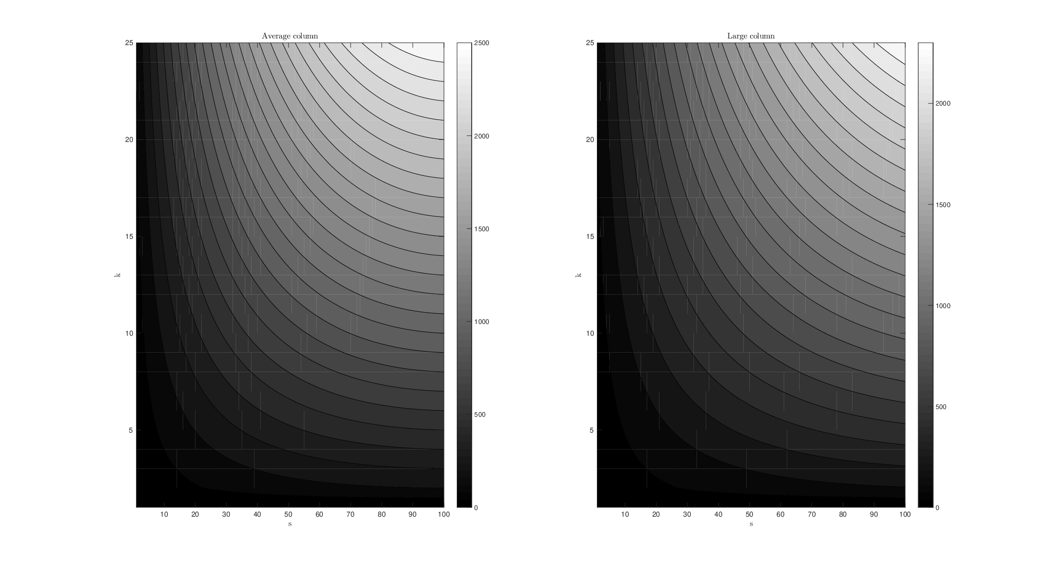
Using computer software, one can calculate mk,s,n,α,β=infτ>0Φk,s,n,α,β​(τ)m_{k,s,n,\alpha,\beta}=\inf_{\tau>0}\Phi_{k,s,n,\alpha,\beta}(\tau). Let us discuss some of the qualitative behaviours one can read out of these numerical evaluations.
Refer to caption
Figure 3: mk,s,n,α,βm_{k,s,n,\alpha,\beta} depending on kk and ss for average (left) and large (right) column. n=100n=100, α=π10\alpha=\tfrac{\pi}{10}.
Refer to caption
Figure 4: The relation between mk,s,n,α,βm_{k,s,n,\alpha,\beta} and mk,s,n,0,0m_{k,s,n,0,0} for k=10k=10, n=100n=100, different values of ss and two types of columns.
Refer to caption
Figure 5: ms,n,k,α,βm_{s,n,k,\alpha,\beta} for k=s=10k=s=10, n=100n=100 depending on α\alpha for two types of columns.

In Figure 3, we fix α=π10\alpha=\tfrac{\pi}{10}, n=100n=100 and plot mk,s,n,α,βm_{k,s,n,\alpha,\beta} for varying kk and ss. We investigate two situations: In the left plot, we set z0​(i∗)‖z0‖1=1s\tfrac{z^{0}(i^{*})}{\|z^{0}\|_{1}}=\tfrac{1}{s} – this corresponds to an ”average size”-column of Z0Z_{0}. In the right, we instead fix z0​(i∗)‖z0‖1=.9\tfrac{z^{0}(i^{*})}{\|z^{0}\|_{1}}=.9 – this corresponds to a large column. With the exception of s=1s=1 (for which 1/s>.91/s>.9), mk,s,n,α,βm_{k,s,n,\alpha,\beta} is larger for the average size column case than for the large column case, as is intuitively clear - it should be easier to recover (the more significant) large columns. We see that the isolines in both plots resemble hyperbolas s⋅k=const.s\cdot k=\text{const.}, which indicates that mk,s,n,α,βm_{k,s,n,\alpha,\beta} scales with s⋅ks\cdot k rather than s+ks+k - that indicates soft recovery needs asymptotically as many measurements as exact recovery. This is also not surprising - after all, the results obtained in this section do not use any low-rank assumptions at all.

In practice however, also non-asymptotic reductions are relevant. This aspect is dealt with in Figure 5, where we fix k=10k=10, n=100n=100, α=π10\alpha=\tfrac{\pi}{10} and plot the quotient mk,s,n,α,βmk,s,n,0,0\tfrac{m_{k,s,n,\alpha,\beta}}{m_{k,s,n,0,0}} - for an average size and large column, respectively. Note that mk,s,n,0,0m_{k,s,n,0,0} exactly corresponds to the threshold amount of measurements needed for exact recovery. Also note that since mk,s,n,α,βm_{k,s,n,\alpha,\beta} only is an upper bound on the amount of measurements needed, it is not a contradiction that it is larger than mk,s,n,0,0m_{k,s,n,0,0} for small values of ss. We see that in particular in the case of a large column, we need considerably less measurements to ensure soft recovery than to ensure exact recovery.

Finally, in Figure 5, we fix k=s=10k=s=10 and n=100n=100 and plot mk,s,n,α,βm_{k,s,n,\alpha,\beta} depending on the size of α\alpha for an average size and large column. We see that at least for small α\alpha, our result provides a smaller upper bound on the measurements needed for soft recovery than for exact recovery. Note that mk,s,n,α,βm_{k,s,n,\alpha,\beta} is growing for large α\alpha (for really large α\alpha, it even surpasses mk,s,n,0,0m_{k,s,n,0,0}. This is again not a contradiction - we have only provided an upper bound, and we already addressed that some of the estimation we make become worse as α\alpha (and therefore also β\beta) grows.

3.2 Energy Concentration

The condition for soft recovery described above is not quite enough to secure that not only the directions, but also the magnitudes, of the columns in the minimizer Z^\widehat{Z} are close to the ones in Z0Z_{0}, but almost. The following proposition holds.

Proposition 3.6.

Let Z0=z0.H0Z_{0}=z_{0}.H_{0} be supported on the set SS and z^.H^\hat{z}.\widehat{H} be the minimizer of the program 𝒫1,2\mathcal{P}_{1,2} with b=𝒜(z0.H0)b=\mathcal{A}(z_{0}.H_{0}). Assume that for each i∈Si\in S, ω⁡(hi0,h^i)≤α\omega(h^{0}_{i},\hat{h}_{i})\leq\alpha, that there for some i∗i^{*} exists a vector p∈ℝmp\in\mathbb{R}^{m} with the properties (3)-(6), and additionally

‖Ai∗​p‖2≤γ,i∉S\displaystyle\|A_{i}^{*}p\|_{2}\leq\gamma,\quad i\notin S (10)

for some γ<1\gamma<1. Then the vector z^\hat{z} obeys

‖z^Sc‖1≤1−cos⁡αcos⁡α⁡(1−γ)​z^i∗\displaystyle\|\hat{z}_{S^{c}}\|_{1}\leq\frac{1-\cos\alpha}{\cos\alpha(1-\gamma)}\hat{z}_{i^{*}} (11)

and

‖z^S−zS0‖2≤sin⁡α​maxi∈S⁡‖Ai‖σℝS​(AH0)​‖z0‖1+maxi∈[n]⁡‖Ai‖σℝS​(AH0)​‖z^Sc‖1.\displaystyle\|\hat{z}_{S}-z^{0}_{S}\|_{2}\leq\sin\alpha\frac{\max_{i\in S}\|A_{i}\|}{\sigma_{\mathbb{R}^{S}}(A_{H_{0}})}\|z_{0}\|_{1}+\frac{\max_{i\in[n]}\|A_{i}\|}{\sigma_{\mathbb{R}^{S}}(A_{H_{0}})}\|\hat{z}_{S^{c}}\|_{1}. (12)

σℝS​(AH0)\sigma_{\mathbb{R}^{S}}(A_{H_{0}}) denotes the to ℝS\mathbb{R}^{S} restricted singular value of AH0A_{H_{0}}, i.e.

σℝS​(AH0)=min‖x‖2=1,supp⁡x⊆S⁡‖AH0​(x)‖2,\displaystyle\sigma_{\mathbb{R}^{S}}(A_{H_{0}})=\min_{\|x\|_{2}=1,\supp x\subseteq S}\|A_{H_{0}}(x)\|_{2},

and ∥⋅∥\|\cdot\| denotes the operator norm.

Proof.

Let us begin by proving (11). Since z^.H^\hat{z}.\widehat{H} obeys the linear constraint, z0.H0−z^.Z^∈ker⁡𝒜=ran⁡𝒜⟂z_{0}.H_{0}-\hat{z}.\widehat{Z}\in\ker\mathcal{A}=\ran\cal A^{\perp}. Consequently, ⟨𝒜∗p,z0.H0−z^.H^⟩=0\left\langle\mathcal{A}^{*}p,z_{0}.H_{0}-\hat{z}.\widehat{H}\right\rangle=0, i.e.

‖z0‖1≤∑i∈S⟨Ai∗​p,zi0​hi0⟩=∑i∈[n]⟨Ai∗​p,z^i​h^i⟩≤1cos⁡α​z^i∗+∑i∈S\{i∗}z^i+γ​∑i∉Sz^i=(1cos⁡α−1)​z^i∗+‖z^S‖1+γ​‖z^Sc‖1\displaystyle\|z_{0}\|_{1}\leq\sum_{i\in S}\left\langle A_{i}^{*}p,z^{0}_{i}h^{0}_{i}\right\rangle=\sum_{i\in[n]}\left\langle A_{i}^{*}p,\hat{z}_{i}\hat{h}_{i}\right\rangle\leq\tfrac{1}{\cos\alpha}\hat{z}_{i^{*}}+\sum_{i\in S\backslash\left\{i^{*}\right\}}\hat{z}_{i}+\gamma\sum_{i\notin S}\hat{z}_{i}=\left(\tfrac{1}{\cos\alpha}-1\right)\hat{z}_{i^{*}}+\|\hat{z}_{S}\|_{1}+\gamma\|\hat{z}_{S^{c}}\|_{1}

We used (3), (6) and (10). At the same time, due to the optimality of z^.H^\hat{z}.\widehat{H}, there must be ‖z^S‖1+‖z^Sc‖1≤‖z0‖1\|\hat{z}_{S}\|_{1}+\|\hat{z}_{S^{c}}\|_{1}\leq\|z_{0}\|_{1}. These two inequalities imply

cos⁡α⁡(1−γ)​‖z^Sc‖1≤(1−cos⁡α)​z^i∗\displaystyle\cos\alpha(1-\gamma)\|\hat{z}_{S^{c}}\|_{1}\leq(1-\cos\alpha)\hat{z}_{i^{*}}

which implies the first half of (11).

To prove the second estimate, we again utilize that 𝒜(z0.H0−z^.H^)=0\mathcal{A}(z_{0}.H_{0}-\hat{z}.\widehat{H})=0. That equation can namely be written

∑i∈SAi∗​hi0​(zi0−z^i)+\displaystyle\sum_{i\in S}A_{i}^{*}h_{i}^{0}(z^{0}_{i}-\hat{z}_{i})+ ∑i∈SAi∗​(hi0−h^i)​z^i−∑i∉Sz^i​Ai∗​h^i=0⇒\displaystyle\sum_{i\in S}A_{i}^{*}(h_{i}^{0}-\hat{h}_{i})\hat{z}_{i}-\sum_{i\notin S}\hat{z}_{i}A_{i}^{*}\hat{h}_{i}=0\Rightarrow
‖AH0​(z0−z^)‖2≤\displaystyle\|A_{H_{0}}(z_{0}-\hat{z})\|_{2}\leq ∑i∈Sz^i​‖Ai∗​(hi0−h^i)‖+∑i∉Sz^i​‖Ai∗​h^i‖\displaystyle\sum_{i\in S}\hat{z}_{i}\|A_{i}^{*}(h_{i}^{0}-\hat{h}_{i})\|+\sum_{i\notin S}\hat{z}_{i}\|A_{i}^{*}\hat{h}_{i}\|
≤\displaystyle\leq ‖z^S‖1​maxi∈S​‖Ai‖​sin⁡(α)+‖z^Sc‖1​maxi∉S​‖Ai‖\displaystyle\|\hat{z}_{S}\|_{1}\max_{i\in S}\|A_{i}\|\sin(\alpha)+\|\hat{z}_{S^{c}}\|_{1}\max_{i\notin S}\|A_{i}\|
≤\displaystyle\leq sin⁡(α)​maxi∈S​‖Ai‖​‖z0‖1+(1−sin⁡α)​maxi∈[n]​‖Ai‖​‖z^Sc‖1\displaystyle\sin(\alpha)\max_{i\in S}\|A_{i}\|\|z_{0}\|_{1}+(1-\sin\alpha)\max_{i\in[n]}\|A_{i}\|\|\hat{z}_{S^{c}}\|_{1}

We utilized that ‖hi0−h^i‖2≤sin⁡α\|h^{0}_{i}-\hat{h}_{i}\|_{2}\leq\sin\alpha for i∈Si\in S and ‖z^S‖=‖z^‖1−‖z^Sc‖1≤‖z0‖1−‖z^Sc‖\|\hat{z}_{S}\|=\|\hat{z}\|_{1}-\|\hat{z}_{S^{c}}\|_{1}\leq\|z_{0}\|_{1}-\|\hat{z}_{S^{c}}\|. To finish the proof, we simply have to note that ‖AH0​(z0−z^S)‖2≥σℝS​(AH0)​‖(z0−z^)S‖2\|A_{H_{0}}(z_{0}-\hat{z}_{S})\|_{2}\geq\sigma_{\mathbb{R}^{S}}(A_{H_{0}})\|(z_{0}-\hat{z})_{S}\|_{2} . ∎

Remark 3.7.

It is known that with high probability, maxi∈[n]⁡‖Ai‖≲m+k\max_{i\in[n]}\|A_{i}\|\lesssim\sqrt{m}+\sqrt{k} and σℝS​(AH0)≳m−s\sigma_{\mathbb{R}^{S}}(A_{H_{0}})\gtrsim\sqrt{m}-\sqrt{s} [8, Th. 9.6]. Hence, if we choose m≥C2​max⁡(s,k)m\geq C^{2}\max(s,k), we can guarantee that

maxi∈[n]⁡‖Ai‖σℝS​(AH0)≤C+1C−1\frac{\max_{i\in[n]}\|A_{i}\|}{\sigma_{\mathbb{R}^{S}}(A_{H_{0}})}\leq\frac{C+1}{C-1}

with high probability.

3.3 Taking Low Rank Into Account.

Until know, all theory has been valid for arbitrary column-sparse matrices. In the following, we will prove that under the assumption that Z0Z_{0} has been softly recovered by the program 𝒫1,2\mathcal{P}_{1,2} and Z0Z_{0} is a certain type of an rr-rank matrix (we will specify the exact requirements on Z0Z_{0} later), the space spanned by the leading rr left singular vectors of the recovered matrix will be close to the true range of Z0Z_{0}. The argumentation will rely heavily on a classical result from pertubation theory; the so-called sin⁡θ\sin\theta-theorem. We will start this section by recalling that theorem. We follow the original paper [16].

Let two matrices AA and B=A+T∈ℝm,nB=A+T\in\mathbb{R}^{m,n} be given. Write the singular value decomposition of AA in the following manner:

A=A1+A2=U1​(A)​Σ1​(A)​V1​(A)∗+U2​(A)​Σ2​(A)​V2​(A)∗\displaystyle A=A_{1}+A_{2}=U_{1}(A)\Sigma_{1}(A)V_{1}(A)^{*}+U_{2}(A)\Sigma_{2}(A)V_{2}(A)^{*}

where the left and right singular vectors of AA are given by the columns of the matrices [U1​(A),U2​(A)][U_{1}(A),U_{2}(A)] and [V1​(A),V2​(A)][V_{1}(A),V_{2}(A)], respectively, and the union of the diagonals of Σ1\Sigma_{1} and Σ2\Sigma_{2} is the set of singular values of AA. The dimensions of the matrices are as follows:

U1​(A)∈ℝm,r,\displaystyle U_{1}(A)\in\mathbb{R}^{m,r},\quad Σ1​(A)∈ℝr,r,V1​(A)∈ℝn,r\displaystyle\Sigma_{1}(A)\in\mathbb{R}^{r,r},\quad V_{1}(A)\in\mathbb{R}^{n,r}
U2​(A)∈ℝm,m−r,\displaystyle U_{2}(A)\in\mathbb{R}^{m,m-r},\quad Σ2​(A)∈ℝm−r,m−r,V2​(A)∈ℝn,m−r\displaystyle\Sigma_{2}(A)\in\mathbb{R}^{m-r,m-r},\quad V_{2}(A)\in\mathbb{R}^{n,m-r}

B1B_{1}, B2B_{2}, U1​(B)U_{1}(B), Σ1​(B)\Sigma_{1}(B) and so on are defined in the same manner. The sin⁡θ\sin\theta-theorem is a statement about the principal angle between the subspaces spanned by U1​(A)U_{1}(A) and U1​(B)U_{1}(B) (and V1​(A)V_{1}(A) and V1​(B)V_{1}(B)). The principal angle ∠⁡(E,F)∈[0,π2]\angle(E,F)\in[0,\tfrac{\pi}{2}] between two subspaces EE and FF are thereby defined through

sin⁡∠⁡(E,F)=‖ΠE⟂​ΠF‖.\displaystyle\sin\angle(E,F)=\|\Pi_{E^{\perp}}\Pi_{F}\|.
Theorem 3.8 (The sin⁡θ\sin\theta-theorem).

[16] Assume the matrices A,BA,B and TT are given as above. Define the parameter μ\mu through

μ=max⁡(‖Πran⁡B1​T‖,‖T​Πker⁡B1⟂‖).\displaystyle\mu=\max(\|\Pi_{\ran B_{1}}T\|,\|T\Pi_{\ker B_{1}^{\perp}}\|).

Further assume that there exists a τ≥0\tau\geq 0 and a δ>0\delta>0 such that

σmin​(A1)≥τ+δ∧σmax​(B2)≤τ.\displaystyle\sigma_{\min}(A_{1})\geq\tau+\delta\ \wedge\ \sigma_{\max}(B_{2})\leq\tau.

Then there holds

max⁡(sin⁡∠⁡(ran⁡A1,ran⁡B1),sin⁡∠⁡(ker⁡A1⟂,ker⁡B1⟂))≤μδ.\displaystyle\max(\sin\angle(\ran A_{1},\ran B_{1}),\sin\angle(\ker A_{1}^{\perp},\ker B_{1}^{\perp}))\leq\frac{\mu}{\delta}.

With the above theory, we can prove the following result. We use the notation ⟨A⟩:=ran⁡A\left\langle A\right\rangle:=\ran A.

Proposition 3.9.

Let the matrix Z0=z0.H0Z_{0}=z_{0}.H_{0} be supported on the set SS and have at most rank rr. Assume furthermore that SS can be partitioned into LL disjoint subsets SℓS_{\ell}, ℓ=1,…,L\ell=1,\dots,L so that

hi0=ηℓ0mod±1,i∈Sℓ\displaystyle h_{i}^{0}=\eta_{\ell}^{0}\mod\pm 1,\quad i\in S_{\ell}

for some unit-norm frame (ηℓ)ℓ∈[L](\eta_{\ell})_{\ell\in[L]} of ⟨H0⟩\langle H_{0}\rangle with lower frame bound Λ\Lambda.

If then Z^=z^.H^\widehat{Z}=\hat{z}.\widehat{H} has the properties that ω⁡(hi0,h^i)≤α<π2\omega(h_{i}^{0},\hat{h}_{i})\leq\alpha<\tfrac{\pi}{2}, we have for the space ⟨H^⟩r\langle\widehat{H}\rangle_{r} spanned by the rr first singular vectors of H^\widehat{H}

sin⁡∠⁡(⟨H^⟩r,⟨H0⟩)≤max⁡(sin⁡α​‖z^S‖2,‖z^Sc‖2)Λ​minℓ​‖z^Sℓ‖22−sin⁡α​‖z^S‖22\displaystyle\sin\angle(\langle\widehat{H}\rangle_{r},\left\langle H_{0}\right\rangle)\leq\frac{\max(\sin\alpha\|\hat{z}_{S}\|_{2},\|\hat{z}_{S^{c}}\|_{2})}{\sqrt{\Lambda\min_{\ell}\|\hat{z}_{S_{\ell}}\|_{2}^{2}-\sin{\alpha}\|\hat{z}_{S}\|_{2}^{2}}}
Proof.

Let ϵ>0\epsilon>0 be arbitrary and define the matrices BB and TT through

B⁡(i)={max⁡(z^i,ϵ)​⟨h^i,hi0⟩​hi0i∈S0i∉ST⁡(i)={z^i​h^i−max⁡(z^i,ϵ)​⟨h^i,hi0⟩​hi0i∈Szi^​h^ii∉S\displaystyle B(i)=\begin{cases}\max(\hat{z}_{i},\epsilon)\left\langle\hat{h}_{i},h^{0}_{i}\right\rangle h^{0}_{i}&i\in S\\ 0&i\notin S\end{cases}\quad T(i)=\begin{cases}\hat{z}_{i}\hat{h}_{i}-\max(\hat{z}_{i},\epsilon)\left\langle\hat{h}_{i},h^{0}_{i}\right\rangle h^{0}_{i}&i\in S\\ \hat{z_{i}}\hat{h}_{i}&i\notin S\end{cases}

Adopting the notation from above, we further set A=z^.H^A=\hat{z}.\widehat{H}. Then A=B+TA=B+T and, continuing to use the notation from above, ⟨A1⟩=⟨H^⟩r\left\langle A_{1}\right\rangle=\langle\widehat{H}\rangle_{r}, ⟨B1⟩=⟨H0⟩\left\langle B_{1}\right\rangle=\left\langle H_{0}\right\rangle. (The latter is due to max⁡(z^i,ϵ)​⟨h^i,hi0⟩≠0\max(\hat{z}_{i},\epsilon)\langle{\hat{h}_{i},h^{0}_{i}}\rangle\neq 0 for all ii, which is a consequence of α<π2\alpha<\tfrac{\pi}{2} and ϵ>0\epsilon>0.) Hence

sin∠(⟨H0⟩,⟨H^⟩r,)=sin∠(⟨A1⟩,⟨B1⟩).\displaystyle\sin\angle(\left\langle H_{0}\right\rangle,\langle\widehat{H}\rangle_{r},)=\sin\angle(\left\langle A_{1}\right\rangle,\left\langle B_{1}\right\rangle).

We now want to apply the sin⁡θ\sin\theta-theorem. Towards this end, we have to estimate the parameters μ\mu, τ\tau and δ\delta. τ\tau can be chosen equal to zero – the range of BB is contained in ⟨H0⟩\left\langle H_{0}\right\rangle, and hence is at most rr-dimensional. Consequently, BB has at most rr non-zero singular values, and B2=0B_{2}=0. To estimate μ\mu, we begin by noting that ker⁡B1⟂=ker⁡B⟂⊆ℝS\ker B_{1}^{\perp}=\ker B^{\perp}\subseteq\mathbb{R}^{S} (since ℝSc⊆ker⁡B\mathbb{R}^{S^{c}}\subseteq\ker B). This implies

‖T​Πker⁡B1⟂‖≤‖T​ΠℝS‖≤sup‖x‖2≤1∑i∈S|xi|​(ϵ​|⟨h^i,hi0⟩|+z^i​‖Π⟨H0⟩⟂​h^i‖2)≤s​ϵ+‖z^S‖2​sin⁡α.\displaystyle\|T\Pi_{\ker B_{1}^{\perp}}\|\leq\|T\Pi_{\mathbb{R}^{S}}\|\leq\sup_{\|x\|_{2}\leq 1}\sum_{i\in S}|x_{i}|(\epsilon|\langle\hat{h}_{i},h_{i}^{0}\rangle|+\hat{z}_{i}\|\Pi_{\left\langle H_{0}\right\rangle^{\perp}}\hat{h}_{i}\|_{2})\leq\sqrt{s}\epsilon+\|\hat{z}_{S}\|_{2}\sin\alpha.

In the last step, we used the Cauchy Schwarz inequality and

‖Π⟨H0⟩⟂​h^i‖2=minv∈⟨H0⟩⁡‖h^i−v‖2≤‖h^i−⟨h^i,hi0⟩​hi0‖2=1−cos2⁡(ω⁡(h^i,hi0))≤sin⁡α\displaystyle\|\Pi_{\left\langle H_{0}\right\rangle^{\perp}}\hat{h}_{i}\|_{2}=\min_{v\in\left\langle H_{0}\right\rangle}\|\hat{h}_{i}-v\|_{2}\leq\|\hat{h}_{i}-\langle{\hat{h}_{i},h_{i}^{0}}\rangle h_{i}^{0}\|_{2}=\sqrt{1-\cos^{2}(\omega(\hat{h}_{i},h_{i}^{0}))}\leq\sin\alpha

due to ω⁡(h^i,hi0)≤α\omega(\hat{h}_{i},h_{i}^{0})\leq\alpha for i∈Si\in S. We also have, since ⟨B1⟩=⟨H0⟩\left\langle B_{1}\right\rangle=\left\langle H_{0}\right\rangle

∥Πran⁡B1T∥=∥z^Sc.(Π⟨H0⟩H^)∥≤∥z^Sc∥2.\displaystyle\|\Pi_{\ran B_{1}}T\|=\|\hat{z}_{S^{c}}.(\Pi_{\left\langle H_{0}\right\rangle}\widehat{H})\|\leq\|\hat{z}_{S^{c}}\|_{2}.

Here we used that the vectors in H^\widehat{H} have unit norm and an argument similar as above. Summarizing,

μ≤max⁡(s​ϵ+sin⁡α​‖z^S‖2,‖z^Sc‖2)\mu\leq\max(\sqrt{s}\epsilon+\sin\alpha\|\hat{z}_{S}\|_{2},\|\hat{z}_{S^{c}}\|_{2})

It remains to estimate the gap δ\delta. Since we already have noted that τ\tau can be chosen equal to zero we mearly need to estimate σmin​(A1)=σr​(A)\sigma_{\min}(A_{1})=\sigma_{r}(A) from below. To do this, we use two well known facts: firstly the equality σr​(A)=σr​(A∗)\sigma_{r}(A)=\sigma_{r}(A^{*}), and secondly the so-called max\max-min\min-principle (or Courant-Fischer Theorem):

σr​(A∗)=maxdimV≤r⁡minp∈V‖p‖2=1​‖A∗​p‖.\displaystyle\sigma_{r}(A^{*})=\max_{\dim V\leq r}\min_{\begin{subarray}{c}p\in V\\ \|p\|_{2}=1\end{subarray}}\|A^{*}p\|.

Hence, since dim⟨H0⟩≤r\dim\left\langle H_{0}\right\rangle\leq r

σr(A∗)≥minp∈⟨H0⟩‖p‖2=1∥(z^.H^)∗p∥2.\displaystyle\sigma_{r}(A^{*})\geq\min_{\begin{subarray}{c}p\in\left\langle H_{0}\right\rangle\\ \|p\|_{2}=1\end{subarray}}\|(\hat{z}.\widehat{H})^{*}p\|_{2}.

The adjoint of z^.H^\hat{z}.\widehat{H} is given by ((z^.H^)p)i=z^i⟨h^i,p⟩((\hat{z}.\widehat{H})p)_{i}=\hat{z}_{i}\langle{\hat{h}_{i},p}\rangle. Hence

∥(z^.H^)∗p∥22=∑i∈[n]z^i2|⟨h^i,p⟩|2≥∑i∈Sz^i2|⟨h^i,p⟩|2\displaystyle\|(\hat{z}.\widehat{H})^{*}p\|_{2}^{2}=\sum_{i\in[n]}\hat{z}_{i}^{2}|\langle{\hat{h}_{i},p}\rangle|^{2}\geq\sum_{i\in S}\hat{z}_{i}^{2}|\langle{\hat{h}_{i},p}\rangle|^{2}

Now we notice that if ‖p‖2=1\|p\|_{2}=1, the following is true due to the triangle inequality of ω\omega and ω⁡(h^i,hi0)≤α\omega(\hat{h}_{i},h_{i}^{0})\leq\alpha

|⟨h^i,p⟩|2=cos2⁡(ω⁡(h^i,p))≥cos2⁡(min⁡(ω⁡(hi0,p)+α,π2))≥cos2⁡(ω⁡(hi0,p))−sin⁡α=|⟨hi0,p⟩|2−sin⁡α,\displaystyle|\langle{\hat{h}_{i},p}\rangle|^{2}=\cos^{2}(\omega(\hat{h}_{i},p))\geq\cos^{2}(\min(\omega(h_{i}^{0},p)+\alpha,\tfrac{\pi}{2}))\geq\cos^{2}(\omega(h_{i}^{0},p))-\sin\alpha=|\langle h^{0}_{i},p\rangle|^{2}-\sin\alpha,

where the proof of the last inequality is postponed to the Appendix (more specifically Lemma A.3). Therefore, we may estimate

∑i∈Sz^i2​|⟨h^i,p⟩|2≥∑i∈Sz^i2​|⟨hi0,p⟩|2−sin⁡(α)​‖z^S‖22\displaystyle\sum_{i\in S}\hat{z}_{i}^{2}|\langle{\hat{h}_{i},p}\rangle|^{2}\geq\sum_{i\in S}\hat{z}_{i}^{2}|\langle{h_{i}^{0},p}\rangle|^{2}-\sin(\alpha)\|\hat{z}_{S}\|_{2}^{2}

Now we utilize the structure of the set (h^i)i∈S(\hat{h}_{i})_{i\in S} to estimate

∑i∈Sz^i2​|⟨hi0,p⟩|2=∑ℓ∈[L]|⟨ηℓ0,p⟩|2​∑i∈Sℓz^i2≥minℓ⁡‖zSℓ‖22​∑ℓ∈[L]|⟨ηℓ0,p⟩|2≥Λ​minℓ​‖zSℓ‖22\displaystyle\sum_{i\in S}\hat{z}_{i}^{2}|\langle{h_{i}^{0},p}\rangle|^{2}=\sum_{\ell\in[L]}|\langle{\eta_{\ell}^{0},p}\rangle|^{2}\sum_{i\in S_{\ell}}\hat{z}_{i}^{2}\geq\min_{\ell}\|z_{S_{\ell}}\|_{2}^{2}\sum_{\ell\in[L]}|\langle{\eta_{\ell}^{0},p}\rangle|^{2}\geq\Lambda\min_{\ell}\|z_{S_{\ell}}\|_{2}^{2}

for all p∈⟨H0⟩p\in\left\langle H_{0}\right\rangle with ‖p‖2\|p\|_{2}. All in all,

δ2≥Λ​minℓ​‖zSℓ‖22−sin⁡(α)​‖z^S‖22,\displaystyle\delta^{2}\geq\Lambda\min_{\ell}\|z_{S_{\ell}}\|_{2}^{2}-\sin(\alpha)\|\hat{z}_{S}\|_{2}^{2},

which together with the sin⁡θ\sin\theta-theorem proves

sin⁡∠⁡(⟨H^⟩r,⟨H0⟩)≤max⁡(ϵ​s+sin⁡α​‖z^S‖2,‖z^Sc‖2)Λ​minℓ​‖z^Sℓ‖22−sin⁡α​‖z^S‖22.\displaystyle\sin\angle(\langle\widehat{H}\rangle_{r},\left\langle H_{0}\right\rangle)\leq\frac{\max(\epsilon\sqrt{s}+\sin\alpha\|\hat{z}_{S}\|_{2},\|\hat{z}_{S^{c}}\|_{2})}{\sqrt{\Lambda\min_{\ell}\|\hat{z}_{S_{\ell}}\|_{2}^{2}-\sin{\alpha}\|\hat{z}_{S}\|_{2}^{2}}}.

Letting ϵ→0\epsilon\to 0 yields the claim. ∎

Remark 3.10.

In the case that r=1r=1, all columns hi0h_{i}^{0}, i∈Si\in S must be equal modulo sign, which implies that we may choose L=1L=1, η10=h10\eta_{1}^{0}=h_{1}^{0}, S1=SS_{1}=S and consequently Λ=1\Lambda=1. We then arrive at the cleaner estimate

sin⁡∠⁡(⟨H^⟩r,⟨H0⟩)≤max⁡(sin⁡α​‖z^S‖2,‖z^Sc‖2)‖z^S‖2​1−sin⁡α.\displaystyle\sin\angle(\langle\widehat{H}\rangle_{r},\left\langle H_{0}\right\rangle)\leq\frac{\max(\sin\alpha\|\hat{z}_{S}\|_{2},\|\hat{z}_{S^{c}}\|_{2})}{\|\hat{z}_{S}\|_{2}\sqrt{1-\sin\alpha}}.

4 Heuristic Proposals How One Could Utilize Soft Recovery

In this section, we will present two ideas how one could use the phenomenon of soft recovery to design a recovery algorithm for matrices which are both column-sparse and have low rank. These ideas are of highly heuristic nature, whence we mostly study them experimentally.

4.1 Thresholding

The above analysis indicates that the set of indices where z^i\hat{z}_{i} is large probably coincides relatively well with the support of z0z_{0}, since ‖z^Sc‖1\|\hat{z}_{S^{c}}\|_{1} is small. Hence, if we choose a set S^\widehat{S} for which ‖Z^S^‖1,2≥‖Z^‖1,2∗τ\|\widehat{Z}_{\widehat{S}}\|_{1,2}\geq\|\widehat{Z}\|_{1,2}*\tau for τ≈1\tau\approx 1 and S^≥s\widehat{S}\geq s, S^\hat{S} is most probably a small set which still contains the support of the ground truth signal Z0Z_{0}. After having identified the support, the remaining task is then to recover a low-rank matrix of dimension k×|S^|k\times|\widehat{S}|, which we choose to do with nuclear norm-minimization minimization. This will be successful with high probability already when m≳r⁡(k+|S^|)​log⁡(k​|S^|)m\gtrsim r(k+|\widehat{S}|)\log(k|\widehat{S}|) [14].

The procedure outlined above is summarized in Algorithm 1.

Algorithm 1 (NAST) Nuclear norm After Soft recovery Thresholding.
Data: A linear map 𝒜:ℝk,n→ℝq\mathcal{A}:\mathbb{R}^{k,n}\to\mathbb{R}^{q}, a sparsity ss, a parameter τ∈(0,1)\tau\in(0,1) and a vector bb.
Result: An estimate Z∗Z_{*} of a sparse solution of 𝒜⁡(Z)=b\mathcal{A}(Z)=b, where Z∗=z∗.H∗Z_{*}=z_{*}.H_{*} with z∗z_{*} sparse and H∗H_{*} low rank.
1 Solve the 𝒫1,2\mathcal{P}_{1,2} for a column-sparse matrix Z^=z^.H^\widehat{Z}=\hat{z}.\widehat{H}.
2 S^←\widehat{S}\leftarrow smallest set SS with at least ss indices so that ‖Z^S‖1,2≥τ​‖Z^‖1,2\|\widehat{Z}_{S}\|_{1,2}\geq\tau\|\widehat{Z}\|_{1,2}.
3 Solve the nuclear minimization problem
minsupp⁡Z⊆S^⁡‖Z‖∗​ subject to ​𝒜​(Z)=b\displaystyle\min_{\supp Z\subseteq\widehat{S}}\|Z\|_{*}\text{ subject to }\mathcal{A}(Z)=b
and output the solution Z∗Z_{*}.

4.1.1 Numerical Experiments

To test the performance of the N​A​S​TNAST-algorithm, we perform a small numerical experiment. For m=100,105,…,300m=100,105,\dots,300, we generate random 1010-column sparse matrices in ℝ10,100\mathbb{R}^{10,100} of the form ∑i=1rhi​zi∗\sum_{i=1}^{r}h_{i}z_{i}^{*} for r=1,2r=1,2 and 55 (in all experiments s=k=10s=k=10, n=100n=100.) The vectors hih_{i} are independent and uniformly distributed on the sphere where as zz has a uniformly drawn random support and normally distributed and independent non-zero entries. We measure these matrices with a randomly drawn Gaussian measurement matrix, and test if N​A​S​TNAST is able to recover the ground truth signal. The minimization problems were solved with help of the M​A​T​L​A​BMATLAB-package cvx [12]. A success is declared if the relative error in Frobenius norm is less than 0.1%0.1\%. This experiment was repeated a hundered times, and the results are depicted in Figure 6. We can clearly see that the N​A​S​TNAST-procedure outperforms ℓ1,2\ell_{1,2}. We also see that the performance is better for low ranks, as expected. We performed a small control experiment for m=300m=300 testing the performance of nuclear norm minimization - out of a hundered trials, there was not a single success.

Refer to caption
Figure 6: Results of numerical performance tests of N​A​S​TNAST.

4.2 ”Column Streamlining”

Another idea, which is a bit more involved, we want to present is the following: If Z0Z_{0} is of rank rr, the columns containing most of the energy of Z^\widehat{Z} all almost lie in an rr-dimensional subspace, not far from ran⁡Z0\ran Z_{0}. Hence, the best rank rr-approximation VV of ran⁡Z^\ran\widehat{Z} should be close to ran⁡Z0\ran Z_{0}.

This information can be used to modify the ℓ1,2\ell_{1,2}-norm to more greatly penalize components of the norms of ZZ not lying in the space VV. We propose the following way of doing this

min⁡‖Z‖+‖ΠV⟂​Z‖1,2​ subject to ​𝒜​(Z)=b.\displaystyle\min\|Z\|+\|\Pi_{V^{\perp}}Z\|_{1,2}\text{ subject to }\mathcal{A}(Z)=b.

The procedure of alternately calculating matrices ZZ and subspaces VV according to the procedure described above is then repeated until some stopping criterion is met. Some heuristic proposals for this criterion are for instance that the difference between iterate ZkZ_{k} and Zk+1Z_{k+1} drops below some threshold ϵ\epsilon, or the same for the (r+1)(r+1):st singular value of ZkZ_{k} (indicating that we have found a low-rank solution), or also the (s+1)(s+1):st largest column (indicating that we have found a sparse solution). Alternatively, one could break the iteration already when, say, 2​s2s columns are larger than some threshold, form a set S^\widehat{S} of the corresponding indices, and solve a low-rank problem with that constraint, as above. The main algorithm is summarized in Algorithm 2. We have chose to call it the Column Streamlining algorithm, since it, when successful, forces the non-zero columns of the iterates to all align in a common, low-dimensional subspace.

Algorithm 2 Column Streamlining
Data: A linear map 𝒜:ℝk,n→ℝm\mathcal{A}:\mathbb{R}^{k,n}\to\mathbb{R}^{m}, a rank rr and a vector bb.
Result: An estimate Y∗Y_{*} of a sparse solution of 𝒜⁡(Y)=b\mathcal{A}(Y)=b, where Y∗=z.HY_{*}=z.H with zz sparse and HH of rank less than rr.
Initalize Y0Y_{0} as the solution of 𝒫1,2\mathcal{P}_{1,2} for 𝒜\mathcal{A} and bb, and VV as the the best rr-dimensional approximation of ran⁡Y0\ran Y_{0}, i.e
V=span⁡(U1,…​Ur),V=\spn(U_{1},\dots U_{r}),
where U​Σ​V∗U\Sigma V^{*} is the S​V​DSVD of Y0Y_{0}.
repeat
    1 YqY_{q} ←\leftarrow argmin⁡‖Y‖1,2+‖ΠVq−1⟂​Y‖1,2\argmin\|Y\|_{1,2}+\|{\Pi_{V_{q-1}^{\perp}}Y}\|_{1,2} subject to 𝒜⁡(Y)=b\mathcal{A}(Y)=b.
    2 VqV_{q} ←\leftarrow The best rr-dimensional approximation of ran⁡Yk\ran Y_{k}.
until A stopping criterion is met;

We cannot report much success about theoretical guarantees about the performance of the Column Streamlining algorithm. We however believe that it again will not perform well using the optimal amount r⁡(s+k)r(s+k) measurement, but instead again get stuck at the (s⋅k)(s\cdot k)–bottleneck. The argument goes as follows: Let us assume that the iterates Yq→Z0Y_{q}\to Z_{0}. Then it is not hard to prove that Z0Z_{0} has to solve the minimization problem

argmin⁡‖Z‖1,2+‖Π⟨H0⟩⟂​Z‖1,2​ subject to ​𝒜​(Z)=b.\displaystyle\argmin\|Z\|_{1,2}+\|{\Pi_{\left\langle H_{0}\right\rangle^{\perp}}Z}\|_{1,2}\text{ subject to }\mathcal{A}(Z)=b. (𝒫1,2,⟨H0⟩\mathcal{P}_{1,2,\left\langle H_{0}\right\rangle})
Refer to caption
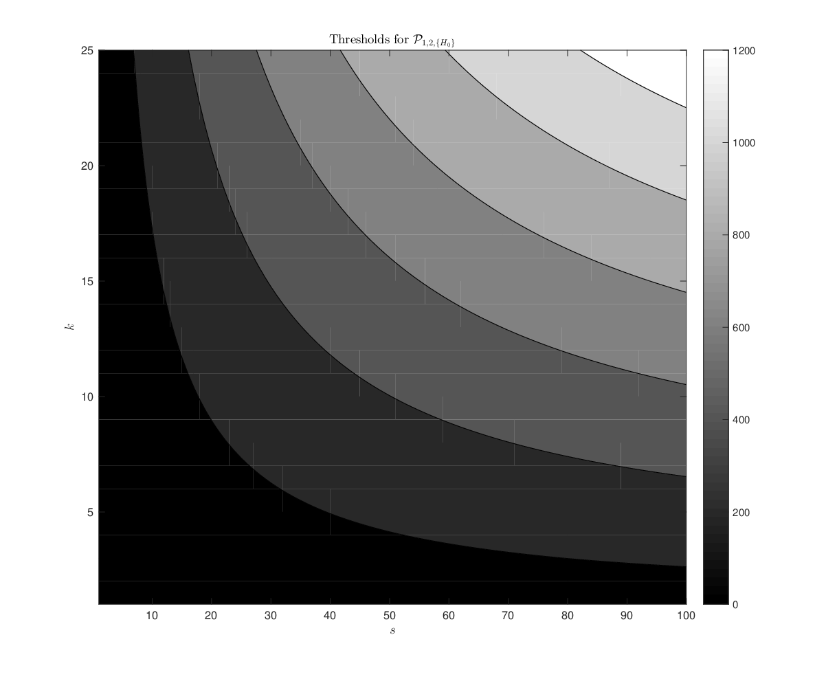
Figure 7: Plot of the function (13) for n=100n=100 and r=1r=1.

By following the exact same route as in Section 3.1 one may now easily prove that an upper bound of the amount of Gaussian measurements needed for the success of the program 𝒫1,2,⟨H0⟩\mathcal{P}_{1,2,\left\langle H_{0}\right\rangle} is given by

μk,s,n,r=infτ>0s⁡(r+τ2+𝔼⁡(pos⁡(‖gk−r‖2−τ)2))+(n−s)​𝔼​(pos⁡(‖gk‖2−τ)2).\displaystyle\mu_{k,s,n,r}=\inf_{\tau>0}s(r+\tau^{2}+\mathbb{E}\left(\pos(\|g^{k-r}\|_{2}-\tau)^{2}\right))+(n-s)\mathbb{E}\left(\pos(\|g^{k}\|_{2}-\tau)^{2}\right). (13)

(The only hard part of the argument, which is to calculate the subdifferential of ∥⋅∥1,2+∥Π⟨H0⟩⟂⋅∥1,2\|\cdot\|_{1,2}+\|{\Pi_{\left\langle H_{0}\right\rangle^{\perp}}\cdot}\|_{1,2}, is presented in Section A.1 of the Appendix.) By plotting this function in Figure 7 for n=100n=100, r=1r=1 for varying values of ss and kk, we see that it scales as s⋅ks\cdot k rather than as s+ks+k. It should however be noted that in absolute numbers, we need considerably less measurements to secure success of 𝒫1,2,⟨H0⟩\mathcal{P}_{1,2,\left\langle H_{0}\right\rangle} than for 𝒫1,2\mathcal{P}_{1,2} - as an example, μ10,10,100,1≈130\mu_{10,10,100,1}\approx 130 whereas m10,10,100,0≈236m_{10,10,100,0}\approx 236

4.2.1 Numerical Experiments

We chose to test the numerical performance of the Column Streamlining algorithm as follows: Matrices were generated as above (i.e. k=s=10k=s=10, n=100n=100) for r=2r=2, for each m=100,101,…,140m=100,101,\dots,140. Then we let the Column Streamlining algorithm perform 1010 iterations, and subsequently recorded the relative difference in Frobenius norm between the final iterate Y∗Y_{*} and the ground truth signal Z0Z_{0}. This was repeated a hundered times for each value of mm. We again used cvx to solve the minimization programs. The number of experiments in which the final relative error was smaller than 0.1%0.1\% and 1%1\%, respectively, are depicted and compared with the results of the N​A​S​TNAST-experiments in Figure 8. We see that the Column Streamlining outperforms the N​A​S​TNAST-approach. The big difference between the number of final iterates with a relative error smaller than 0.1%0.1\% and 1%1\% suggest that better results if we let the algorithm perform more iterations.

Refer to caption
Figure 8: Numerical results of the Column Streamlining Algorithm.

Acknowledgement

The author acknowledges support from Deutsche Forschungsgemeinschaft (DFG) Grant KU 1446/18 - 1 and Berlin Mathematical School. He also likes to thank Gitta Kutyniok, Saeid Haghighatshoar and Peter Jung for interesting discussions on this and other topics.

References

  • [1] A. Ahmed, B. Recht, and J. Romberg. Blind deconvolution using convex programming. IEEE Trans. Inf. Theory, 60(3):1711–1732, 2014.
  • [2] D. Amelunxen, M. Lotz, M. B. McCoy, and J. A. Tropp. Living on the edge: phase transitions in convex programs with random data. Information and Inference, 3:224 – 294, 2014.
  • [3] S. Boyd and L. Vanderberghe. Convex Optimization. Cambridge University Press, 7th edition, 2009.
  • [4] E. Candès and T. Tao. Decoding by linear programming. IEEE Trans. Inf. Theory, 51:4203–4215, 2005.
  • [5] D. Donoho and J. Tanner. Sparse nonnegative solution of underdetermined linear equations by linear programming. Proc. Natl. Acad. Sci. USA, 102:9446–9451, 2005.
  • [6] Y. Eldar and M. Mishali. Robust recovery of signals from a structured union of subspaces. IEEE Trans. Inf. Theory, 55(11):5302–5316, Nov 2009.
  • [7] A. Flinth and G. Kutyniok. P​R​O​M​PPROMP: A Sparse Recovery Approach to Lattice-Valued Signals. 2016. Preprint.
  • [8] S. Foucart and H. Rauhut. A mathematical introduction to Compressed Sensing. Birkhäuser, 2013.
  • [9] Y. Gordon. On Milman’s inequality and random subspaces which escape through a mesh in ℝn\mathbb{{R}}^{n}. In J. Lindenstrauss and V. D. Milman, editors, Geometric Aspects of Functional Analysis, volume 1317 of Lecture Notes in Mathematics, pages 84–106. Springer Berlin Heidelberg, 1988.
  • [10] J. P. Haldar and D. Hernando. Rank-constrained solutions to linear matrix equations using powerfactorization. IEEE Signal Processing Lett., 16(7):584–587, 2009.
  • [11] K. Lee, Y. Wu, and Y. Bresler. Near optimal compressed sensing of sparse rank-one matrices via sparse power factorization. arXiv preprint arXiv:1312.0525, 2013.
  • [12] M. MGrant and S. Boyd. CVX: Matlab software for disciplined convex programming, version 2.1. http://cvxr.com/cvx, Mar. 2014.
  • [13] S. Oymak, A. Jalali, M. Fazel, Y. C. Eldar, and B. Hassibi. Simultaneously structured models with application to sparse and low-rank matrices. IEEE Trans. Inf. Theory, 61(5):2886–2908, 2015.
  • [14] B. Recht, M. Fazel, and P. A. Parrilo. Guaranteed minimum-rank solutions of linear matrix equations via nuclear norm minimization. SIAM review, 52(3):471–501, 2010.
  • [15] M. Stojnic, F. Parvaresh, and B. Hassibi. On the reconstruction of block-sparse signals with an optimal number of measurements. IEEE Trans. Signal Process., 57(8):3075–3085, 2009.
  • [16] P.-Å. Wedin. Perturbation bounds in connection with singular value decomposition. BIT Numerical Mathematics, 12(1):99–111, 1972.
  • [17] P. Wojtaszczyk. Stability and instance optimality for gaussian measurements in compressed sensing. Found. Comput. Math., 10(1):1–13, 2010.

Appendix A Appendix

We here provide minor proofs not contained in the main body of the article. We begin with the argument advertised in the introduction about the impossibility of soft recovery via ℓ1\ell_{1}-minimization.

Proposition A.1.

Let A∈ℝm,nA\in\mathbb{R}^{m,n} and z0∈ℝnz_{0}\in\mathbb{R}^{n} be arbitrary. If ℓ1\ell_{1}-minimization problem 𝒫1\mathcal{P}_{1} with b=A​z0b=Az_{0} has a unique solution z∗z_{*}, one of the following alternatives hold

  • •

    z0=z∗z_{0}=z_{*}

  • •

    z∗​(i)=0z_{*}(i)=0 for at least one i∈supp⁡z0i\in\supp z_{0} .

Proof.

Denote supp⁡z∗=S∗\supp z^{*}=S^{*}. Towards a contradiction, assume that z0≠z∗z_{0}\neq z_{*} and that the support SS of z0z_{0} is contained in S∗S_{*}. By [7, Lem. 5.1] (which little more than a specification of [5, Thm. 1]), z∗‖z∗‖1\tfrac{z_{*}}{\|z_{*}\|_{1}} then necessarily lies in the relative interior of an (|S∗|−1)(|S^{*}|-1)-face FF of the crosspolytope

C1={x∈ℝn|‖x‖1≤1}C_{1}=\left\{x\in\mathbb{R}^{n}\ |\ \|x\|_{1}\leq 1\right\}

which is mapped to an (|S∗|−1)(|S^{*}|-1)-face of A​C1AC_{1}. In particular, the columns (ai)(a_{i}) of AA corresponding to i∈S∗i\in S^{*} are linearly independent. But due to the linear constraint, we have

b=∑i∈Sz0​(i)​ai=∑i∈S∗z∗​(i)​ai.\displaystyle b=\sum_{i\in S}z_{0}(i)a_{i}=\sum_{i\in S^{*}}z_{*}(i)a_{i}.

This equation, together with S⊆S∗S\subseteq S_{*} and the linear independence, readily implies z0=z∗z_{0}=z_{*}. ∎

Next, we calculate the dual problem of 𝒫1+\mathcal{P}_{1}^{+}, as was needed in the proof of Lemma 2.2. Note that this calculation is relatively standard, but we include it for completeness.

Lemma A.2.

The dual problem of

min⁡‖z‖1=∑i∈[n]zi​ subject to ​A​x=b,x≥0\displaystyle\min\|z\|_{1}=\sum_{i\in[n]}z_{i}\text{ subject to }Ax=b\ ,\ x\geq 0

is equivalent to

max⁡⟨b,p⟩​ subject to ​A∗​p≤𝟙,\displaystyle\max\left\langle b,p\right\rangle\text{ subject to }A^{*}p\leq\mathds{1},

where 𝟙\mathds{1} is the vector consisting only of entries equal to 11

Proof.

Let us begin by writing the Lagrange dual

ℒ⁡(z,p,μ)=‖z‖1+⟨p,b−A​z⟩−⟨μ,z⟩=⟨b,p⟩+‖z‖1−⟨z,A∗​z+μ⟩\displaystyle\mathcal{L}(z,p,\mu)=\|z\|_{1}+\left\langle p,b-Az\right\rangle-\left\langle\mu,z\right\rangle=\left\langle b,p\right\rangle+\|z\|_{1}-\left\langle z,A^{*}z+\mu\right\rangle

We see that infzℒ⁡(z,p,μ)\inf_{z}\mathcal{L}(z,p,\mu) is finite exactly when ‖A∗​p+μ‖∞≤1\|A^{*}p+\mu\|_{\infty}\leq 1, in which case it is equal to ⟨b,p⟩\left\langle b,p\right\rangle. The dual problem is hence

maxp,μ≥0⁡⟨b,p⟩​ subject to ​‖A∗​p+μ‖∞≤1.\displaystyle\max_{p,\mu\geq 0}\left\langle b,p\right\rangle\text{ subject to }\|A^{*}p+\mu\|_{\infty}\leq 1.

Due to the fact that there exists a μ≥0\mu\geq 0 with ‖A∗​p+μ‖≤1\|A^{*}p+\mu\|\leq 1 if and only if A∗​p≤𝟙A^{*}p\leq\mathds{1}, we see the stated equivalence. ∎

Finally, we prove the trigonometric inequality used in the proof of Proposition 3.9.

Lemma A.3.

For x∈[0,π]x\in[0,\pi] and α∈[0,π2]\alpha\in[0,\tfrac{\pi}{2}], we have

cos2⁡(min⁡(x+α,π2))≥cos2⁡(x)−sin⁡α\displaystyle\cos^{2}\left(\min\left(x+\alpha,\tfrac{\pi}{2}\right)\right)\geq\cos^{2}(x)-\sin\alpha
Proof.

We treat the cases x+α≤π2x+\alpha\leq\tfrac{\pi}{2} and x+α≥π2x+\alpha\geq\tfrac{\pi}{2} separately. In the first case, we have

cos2⁡(min⁡(x+α,π2))\displaystyle\cos^{2}\left(\min\left(x+\alpha,\tfrac{\pi}{2}\right)\right) =cos2⁡(x+α)=(cos⁡(x)​cos⁡(α)−sin⁡(x)​sin⁡(α))2\displaystyle=\cos^{2}(x+\alpha)=(\cos(x)\cos(\alpha)-\sin(x)\sin(\alpha))^{2}
=cos2⁡(x)​cos2⁡(α)−2​cos⁡(x)​sin⁡(x)​cos⁡(α)​sin⁡(α)+sin2⁡(x)​sin2⁡(α)\displaystyle=\cos^{2}(x)\cos^{2}(\alpha)-2\cos(x)\sin(x)\cos(\alpha)\sin(\alpha)+\sin^{2}(x)\sin^{2}(\alpha)
=cos2⁡(x)−sin⁡(α)​((cos2⁡(x)−sin2⁡(x))​sin⁡(α)+2​cos⁡(x)​sin⁡(x)​cos⁡(α))\displaystyle=\cos^{2}(x)-\sin(\alpha)\left((\cos^{2}(x)-\sin^{2}(x))\sin(\alpha)+2\cos(x)\sin(x)\cos(\alpha)\right)
=cos2⁡(x)−sin⁡(α)​(cos⁡(2​x)​sin⁡(α)+sin⁡(2​x)​cos⁡(α))\displaystyle=\cos^{2}(x)-\sin(\alpha)\left(\cos(2x)\sin(\alpha)+\sin(2x)\cos(\alpha)\right)
=cos2⁡(x)−sin⁡(α)​sin⁡(2​x+α)≥cos2⁡(x)−sin⁡(α).\displaystyle=\cos^{2}(x)-\sin(\alpha)\sin(2x+\alpha)\geq\cos^{2}(x)-\sin(\alpha).

In the second case, we may argue as follows: α\alpha and π2\tfrac{\pi}{2} both lie in the interval [−π2,π2][-\tfrac{\pi}{2},\tfrac{\pi}{2}], in which sin\sin is increasing. The inequality α≥π2−x\alpha\geq\tfrac{\pi}{2}-x therefore implies sin⁡(α)≥sin⁡(π2−x)=cos⁡(x)\sin(\alpha)\geq\sin\left(\tfrac{\pi}{2}-x\right)=\cos(x). Hence

cos2⁡(x)−sin⁡(α)≤cos2⁡(x)−cos⁡(x)≤0=cos2⁡(min⁡(x+α,π2)),\displaystyle\cos^{2}(x)-\sin(\alpha)\leq\cos^{2}(x)-\cos(x)\leq 0=\cos^{2}\left(\min\left(x+\alpha,\tfrac{\pi}{2}\right)\right),

which proves the claim. ∎

A.1 The Subdifferential of the Norm Used In 𝒫1,2,⟨H0⟩\mathcal{P}_{1,2,\left\langle H_{0}\right\rangle}

Here we provide the calculation of the subdifferential of ∥⋅∥1,2+∥Π⟨H0⟩⟂⋅∥1,2\|\cdot\|_{1,2}+\|{\Pi_{\left\langle H_{0}\right\rangle^{\perp}}\cdot}\|_{1,2} at Z0Z_{0}, as was advertised in 4.2.

Proposition A.4.

Let Z0=z0.H0Z_{0}=z_{0}.H_{0} be supported on the set SS. Then the subdifferential of ∥⋅∥1,2+∥Π⟨H0⟩⟂⋅∥1,2\|\cdot\|_{1,2}+\|\Pi_{\left\langle H_{0}\right\rangle^{\perp}}\cdot\|_{1,2} at Z0Z_{0} is given by the set of matrices VV for which

V⁡(i)\displaystyle V(i) ∈hi0+B1​(0)∩⟨H0⟩⟂,i∈S\displaystyle\in h_{i}^{0}+B_{1}(0)\cap\left\langle H_{0}\right\rangle^{\perp},\quad i\in S
V⁡(i)\displaystyle V(i) ∈B1​(0)+B1​(0)∩⟨H0⟩⟂,i∉S.\displaystyle\in B_{1}(0)+B_{1}(0)\cap\left\langle H_{0}\right\rangle^{\perp},\quad i\notin S.
Proof.

We are looking for the set of matrices VV for which

∑i∈S‖hi0+U⁡(i)‖2+‖Π⟨H0⟩⟂​U​(i)‖2+∑i∉S‖U⁡(i)‖2+‖Π⟨H0⟩⟂​U​(i)‖2≥∑i∈S‖hi0‖2+⟨V⁡(i),U⁡(i)⟩+∑i∉S⟨V⁡(i),U⁡(i)⟩\displaystyle\sum_{i\in S}\|h_{i}^{0}+U(i)\|_{2}+\|\Pi_{\left\langle H_{0}\right\rangle^{\perp}}U(i)\|_{2}+\sum_{i\notin S}\|U(i)\|_{2}+\|\Pi_{\left\langle H_{0}\right\rangle^{\perp}}U(i)\|_{2}\geq\sum_{i\in S}\|h_{i}^{0}\|_{2}+\left\langle V(i),U(i)\right\rangle+\sum_{i\notin S}\left\langle V(i),U(i)\right\rangle

for all U∈ℝk,nU\in\mathbb{R}^{k,n}. We used that hi0∈⟨H0⟩h_{i}^{0}\in\left\langle H_{0}\right\rangle for all i∈Si\in S. Since the columns of UU can be chosen independently, we can treat each index separately. In the following, we drop the indices in the calculations for notational simplification, and use lower case letters to denote columns of VV and UU, respectively.

Case 1: i∈Si\in S. We aim to characterize the vectors v∈ℝkv\in\mathbb{R}^{k} for which

‖h0+u‖2+‖Π⟨H0⟩⟂​u‖2≥‖h0‖2+⟨v,u⟩\displaystyle\|h^{0}+u\|_{2}+\|\Pi_{\left\langle H_{0}\right\rangle^{\perp}}u\|_{2}\geq\|h^{0}\|_{2}+\left\langle v,u\right\rangle (14)

for all vectors u∈ℝku\in\mathbb{R}^{k}. If v∈h0+B1​(0)∩⟨H0⟩⟂v\in h^{0}+B_{1}(0)\cap\left\langle H_{0}\right\rangle^{\perp}, (14) is satisfied:

‖h0‖2+⟨v,u⟩=‖h0‖2+⟨h0,Π⟨H0⟩​u⟩+⟨Π⟨H0⟩⟂​v,Π⟨H0⟩⟂​u⟩\displaystyle\|h^{0}\|_{2}+\left\langle v,u\right\rangle=\|h^{0}\|_{2}+\left\langle h^{0},\Pi_{\left\langle H_{0}\right\rangle}u\right\rangle+\left\langle\Pi_{\left\langle H_{0}\right\rangle^{\perp}}v,\Pi_{\left\langle H_{0}\right\rangle^{\perp}}u\right\rangle ≤‖h0+Π⟨h0⟩​u‖2+‖Π⟨H0⟩⟂​u‖2\displaystyle\leq\|h^{0}+\Pi_{\left\langle h^{0}\right\rangle}u\|_{2}+\|\Pi_{\left\langle H_{0}\right\rangle^{\perp}}u\|_{2}
≤‖h0+u‖2+‖Π⟨H0⟩⟂​u‖2.\displaystyle\leq\|h^{0}+u\|_{2}+\|\Pi_{\left\langle H_{0}\right\rangle^{\perp}}u\|_{2}.

We now only need to argue that (14) implies that v∈h0+B1​(0)∩⟨H0⟩⟂v\in h^{0}+B_{1}(0)\cap\left\langle H_{0}\right\rangle^{\perp}. By plugging in ±h0\pm h^{0} for uu, we see that

⟨h0,v⟩=‖h0‖2.\displaystyle\left\langle h^{0},v\right\rangle=\|h^{0}\|_{2}.

Hence, vv is of the form h0+v1+v2h^{0}+v_{1}+v_{2} for v1∈⟨H0⟩v_{1}\in\left\langle H_{0}\right\rangle, v1⟂h0v_{1}\perp h^{0} and v2⟂⟨H0⟩v_{2}\perp\left\langle H_{0}\right\rangle. Now, by plugging in λ​v1\lambda v_{1} with λ>0\lambda>0 for uu, we obtain

‖h0‖2+λ​‖v1‖22≤‖h0+λ​v1‖2=‖h0‖22+λ2​‖v1‖22⇒‖v1‖2≤‖h0‖22+λ2​‖v1‖22−‖h0‖2λ,λ>0\displaystyle\|h^{0}\|_{2}+\lambda\|v_{1}\|_{2}^{2}\leq\|h^{0}+\lambda v_{1}\|_{2}=\sqrt{\|h^{0}\|_{2}^{2}+\lambda^{2}\|v_{1}\|_{2}^{2}}\Rightarrow\|v_{1}\|^{2}\leq\frac{\sqrt{\|h^{0}\|_{2}^{2}+\lambda^{2}\|v_{1}\|_{2}^{2}}-\|h^{0}\|_{2}}{\lambda},\lambda>0

By letting λ→0\lambda\to 0, we obtain ‖v1‖2=0\|v_{1}\|_{2}=0. Similarly, plugging in λ​v2\lambda v_{2} for uu, we obtain

‖h0‖+λ​‖v2‖22≤‖h0+λ​v2‖2+λ​‖v2‖2⇒(‖v2‖22−‖v2‖2)≤‖h0‖22+λ2​‖v2‖22−‖h0‖2λ,λ>0.\displaystyle\|h^{0}\|+\lambda\|v_{2}\|_{2}^{2}\leq\|h^{0}+\lambda v_{2}\|_{2}+\lambda\|v_{2}\|_{2}\Rightarrow(\|v_{2}\|_{2}^{2}-\|v_{2}\|_{2})\leq\frac{\sqrt{\|h^{0}\|_{2}^{2}+\lambda^{2}\|v_{2}\|_{2}^{2}}-\|h^{0}\|_{2}}{\lambda},\lambda>0.

Again by letting λ→0\lambda\to 0, we obtain (‖v2‖22−‖v2‖2)≤0(\|v_{2}\|_{2}^{2}-\|v_{2}\|_{2})\leq 0, which only is satisfied if ‖v2‖2≤1\|v_{2}\|_{2}\leq 1.

Case 2: i∉Si\notin S. Here the aim is to characterize the vectors vv for which

‖u‖2+‖Π⟨H0⟩⟂​u‖2≥⟨v,u⟩\displaystyle\|u\|_{2}+\|\Pi_{\left\langle H_{0}\right\rangle^{\perp}}u\|_{2}\geq\left\langle v,u\right\rangle (15)

is true for every u∈ℝku\in\mathbb{R}^{k}. It is not hard to see that (15) is satisfied for every vv of the form w1+w2w_{1}+w_{2} with ‖w1‖2≤1\|w_{1}\|_{2}\leq 1 and ‖w2‖2≤1\|w_{2}\|_{2}\leq 1, w2⟂⟨H0⟩w_{2}\perp\left\langle H_{0}\right\rangle.

To see that (15) implies that vv can be written as claimed is a bit more tricky. It is clear that we can always write vv in the form μ​η1+λ​η2\mu\eta_{1}+\lambda\eta_{2} with η1∈⟨H0⟩\eta_{1}\in\left\langle H_{0}\right\rangle and η2⟂⟨H0⟩\eta_{2}\perp\left\langle H_{0}\right\rangle both having unit norm. Hence, v=(μ​η1+(λ−1)​η2)+η2v=(\mu\eta_{1}+(\lambda-1)\eta_{2})+\eta_{2} and the proof is finished as soon as we have argued that μ2+(λ−1)2≤1\mu^{2}+(\lambda-1)^{2}\leq 1. However, plugging in μ​η1+(λ−1)​η2\mu\eta_{1}+(\lambda-1)\eta_{2} for uu in (15) yields

μ2+(λ−1)2+(λ−1)≥μ2+λ⁡(λ−1)⇒μ2+(λ−1)2≥μ2+(λ−1)2,\displaystyle\sqrt{\mu^{2}+(\lambda-1)^{2}}+(\lambda-1)\geq\mu^{2}+\lambda(\lambda-1)\Rightarrow\sqrt{\mu^{2}+(\lambda-1)^{2}}\geq\mu^{2}+(\lambda-1)^{2},

which implies μ2+(λ−1)2≤1\mu^{2}+(\lambda-1)^{2}\leq 1. ∎