On Riemann’s Paper, “On the Number of Primes Less Than a Given Magnitude”

Bernhard Riemann was born in Breselenz near Dannenberg in Lower Saxony in 1826. Like his father, he was first supposed to become a pastor, but already in high school Riemann’s extraordinary mathematical talent caught the attention of his principal. It is said that Riemann read the 859-page book by Legendre on number theory which was loaned to him by the principal in one week. He began studying mathematics in Göttingen, where he attended lectures by Gauß, although they were closed to first-semester students. Riemann then transferred to Jacobi and Dirichlet in Berlin, both of whom supported and encouraged him; he then returned to Göttingen. His doctoral thesis was on the theory of functions. In order to be permitted to teach as private lecturer in Göttingen, candidates had to submit three suggestions for the topic of their Habilitation lecture, and normally the department head would choose the uppermost topic on the list. Riemann’s third topic was “Basics of Geometry”, and when Gauß read that, he, as department head, selected that topic for Riemann’s Habilitation lecture. Very much surprised, Riemann put all his research on the topic “Electricity, Magnetism, Light and Graviation” aside and in 1854, two months before his trial lecture, created the foundations of differential geometry. Gauß was thrilled! In 1855 Gauß died and was followed by Dirichlet. When Dirichlet died four years later, Riemann took over the mathematics chair at Göttingen University. In 1862, he married Elise Koch, with whom he had one daughter. Riemann fell ill with TB and looked for relief in the milder climate of Tessin, where he died at the early age of only 39 at Lake Maggiore.

In addition to founding differential geometry, Riemann made other major contributions; especially important was his work in the theory of functions; his “Über die Anzahl der Primzahlen unter einer gegebenen Größe” (On the Number of Primes up to a Given Magnitude), communicated in the “Monatsberichte der Berliner Akademie, November 1859, with findings on the zeta function; his works on the theory of integration, the Fourier transformation, the hypergeometric differential equation, and the hyperbolic differential equations and stability problems of solutions of partial differential equations in mathematical physics. Riemann was influenced by the research on algebraic geometry and topology by his Italian mathematician friends Betti and Beltrami. Einstein’s General theory of Relativity would be unthinkable without Riemannian Geometry.

All these topics have kept mathematicians and theoretical physicists busy for many years and will continue to do so for many more to come. Today, exactly 150 years after Riemann’s death, the major unsolved problem in pure mathematics is the so-called Riemann hypothesis, a conjecture made by Riemann in 1859 in his paper on the number of primes less than a given positive integer $x$.

Mathematicians later realized that Riemann’s hypothesis governs the distribution of prime numbers to an extraordinary extent, which is why its proof is so eagerly sought. Since all the efforts of some of the best mathematicians have failed so far, perhaps another Riemann is needed.

This is also true for many local relativistic quantum field theory models of elementary particles, where Riemann’s results are of utmost importance for handling infinities with the aid of his zeta-function regularization. In non-relativistic quantum mechanics, we need a Riemannian Hamiltonian which becomes diagonalized in the prime number basis. The measurement process, i.e., the operator acting on an object that will provide us with such a set of discrete prime number eigenvalues, is still to be found. One might wonder what kind of symmetry structure lies behind this kind of physical system.

Let us not forget that the few papers that Riemann published in his lifetime dealt with physics problems. Moreover, in the days of Gauss, Dirichlet and Riemann, a distinction between the disciplines of mathematics and physics was not made. In particular, Riemann approached problems in mathematics and physics not so much as an analyst but illuminated them globally from a geometric and topological viewpoint, meaning that he made many results of analysis better understood using the new methods of the theory of functions and analytical continuation into the whole complex plane, thereby simplifying many problems of real analysis.

There is a very close connection between the sums of the reciprocals of the integers raised to a variable power that Euler wrote down in 1737, the now-called zeta function,

$$\zeta(s)=\sum\limits^{\infty}_{n=1}\frac{1}{n^{s}}=1+\frac{1}{2^{s}}+\frac{1}{3^{s}}+\frac{1}{4^{s}}+\frac{1}{5^{s}}+\cdots\,,\quad\quad s>1$$

(1)

and the primes - which, as integers, are the very signature of discontinuity. Euler considered $s$ to be a real integer variable with $s>1$ to insure convergence of the sum. Multiplying the definition of $\zeta(s)$ by ${1/2}^{s}$ we obtain

$$\frac{1}{2^{s}}\zeta(s)=\sum\limits^{\infty}_{n=1}\frac{1}{(2n)^{s}}=\frac{1}{2^{s}}+\frac{1}{4^{s}}+\frac{1}{6^{s}}+\frac{1}{8^{s}}+\cdots\,$$

(2)

and subtracting this from $\zeta(s)$ we get

	$\displaystyle\zeta(s)-\frac{1}{2^{s}}\zeta(s)$	$\displaystyle=\sum\limits^{\infty}_{n=1}\frac{1}{n^{s}}-\sum\limits^{\infty}_{n=1}\frac{1}{(2n)^{s}}$
	$\displaystyle\mbox{or}\quad\quad\left(1-\frac{1}{2^{s}}\right)\zeta(s)$	$\displaystyle=1+\frac{1}{3^{s}}+\frac{1}{5^{s}}+\frac{1}{7^{s}}+\frac{1}{9^{s}}+\frac{1}{11^{s}}+\cdots\,.$		(3)

Hence all the multiples of the prime $n=2$ disappeared from the original sum of the defined $\zeta(s)$. In short, we found

$$\left(1-\frac{1}{2^{s}}\right)\zeta(s)=\sum\limits^{\infty}_{n=1\atop\Lambda n\neq 2k}\frac{1}{n^{s}}\,.$$

(4)

Next, we multiply this last result by $1/3^{s}$ to obtain

$$\frac{1}{3^{s}}\left(1-\frac{1}{2^{s}}\right)\zeta(s)=\sum\limits^{\infty}_{n=1\atop\Lambda n\neq 2k}\frac{1}{(3n)^{s}}=1+\frac{1}{3^{s}}+\frac{1}{9^{s}}+\frac{1}{15^{s}}+\frac{1}{21^{s}}+\cdots$$

(5)

and so, subtracting this from $(1-1/2^{s})\zeta(s)$, we have

	$\displaystyle\left(1-\frac{1}{2^{s}}\right)\left(1-\frac{1}{3^{s}}\right)\zeta(s)$	$\displaystyle=1+\frac{1}{5^{s}}+\frac{1}{7^{s}}+\frac{1}{11^{s}}+\cdots$
		$\displaystyle=\sum\limits^{\infty}_{\begin{array}[]{c}n=1\\ \Lambda n\neq 2k\\ \Lambda n\neq 3k\end{array}}\frac{1}{n^{s}}\,.$

Now we multiply this result by $1/5^{s}$ and so on. As we repeat this process over and over, multiplying through our last result by $1/p^{s}$, where $p$ denotes successive primes, we subtract out all the multiples of the primes. Hence, since all integers are composed of primes (Euclid’s fundamental theorem of the theory of numbers), we removed all numbers of the right-hand side of the defining sum of $\zeta(s)$ - except for the number 1. Thus our final result is the product

$$\left\{\Pi_{p\,\mbox{\scriptsize prime}}\left(1-p^{-s}\right)\right\}\zeta(s)=1$$

(9)

or

$$\boxed{\zeta(s)=\Pi_{p\,\mbox{\scriptsize prime}}\frac{1}{1-p^{-s}}=\sum\limits^{\infty}_{n=1}\frac{1}{n^{s}}\,,\quad\quad s>1}\,.$$

(10)

Euler’s actual statement reads: “Si ex serie numerorum primorum sequens formetur expressio $\prod\limits_{p}\frac{p^{s}}{(p^{s}-1)}$ erit eius valor aequalis summae huius seriei $\sum\limits_{n=1}\frac{1}{n^{s}}$.”

Now we are going to extend Euler’s zeta function into the complex plane $C$, which is a major achievement of Riemann’s. Hence from now on, s is complex valued and we write

$$\zeta(s)=\sum\limits^{\infty}_{n=1}\frac{1}{n^{s}}=\frac{1}{1^{2}}+\frac{1}{2^{2}}+\frac{1}{3^{2}}+\cdots\quad\quad\mbox{but with}\quad Re(s)>1\,.$$

(11)

This is an absolutely convergent infinite series, which also holds true for the product of all primes in

$$\zeta(s)=\Pi_{p\,\mbox{\scriptsize prime}}\frac{1}{1-p^{-s}}=\left(\frac{1}{1-2^{-s}}\right)\cdot\left(\frac{1}{1-3^{-s}}\right)\cdot\left(\frac{1}{1-5^{-s}}\right)\cdots\left(\frac{1}{1-p^{-s}}\right)\cdots\,.$$

(12)

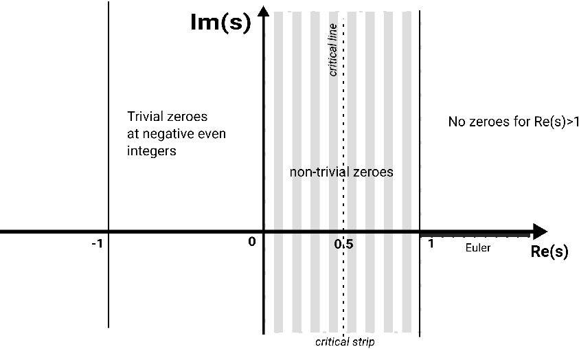
$\zeta(s)$ has no zeros in the region $Re(s)>1$, as none of these factors have zeros. However, with Riemann’s extension of zeta into the entire complex plane, we will be able to locate zeros as well as poles. To show this, we have to analytically continue Euler’s original real valued zeta function into the entire complex $s$ plane. A first result in this direction will be achieved with the aid of the so-called Dirichlet series, which turns up when calculating

	$\displaystyle(1-2^{1-s})\zeta(s)$	$\displaystyle=\sum\limits^{\infty}_{n=1}n^{-s}-2^{1-s}\sum\limits^{\infty}_{n=1}n^{-s}=\sum\limits^{\infty}_{n=1}n^{-s}-2\sum\limits^{\infty}_{n=1}(2n)^{-s}$
		$\displaystyle=1-\frac{2}{2^{s}}+\frac{1}{2^{s}}-\frac{2}{4^{s}}+\cdots=1-\frac{1}{2^{s}}+\frac{1}{3^{s}}-\frac{1}{4^{s}}+\frac{1}{5^{s}}-\frac{1}{6^{s}}+\cdots$
		$\displaystyle=\sum\limits^{\infty}_{n=1}\frac{(-1)^{n+1}}{n^{s}}=:\eta(s)\,,\quad\quad\mbox{Dirichlet series}\,.$		(13)

This series is convergent for all $s\in C$ with $Re(s)>0$. Hence we can define

$$\boxed{\zeta(s)=\frac{1}{1-2^{1-s}}\sum\limits^{\infty}_{n=1}\frac{(-1)^{n+1}}{n^{s}}\quad\quad\mbox{for}\quad Re(s)>0\quad\mbox{and}\quad 1-2^{1-s}\neq 0\,.}$$

(14)

When we write

	$\displaystyle\eta(s)+\frac{2}{2^{s}}\zeta(s)$	$\displaystyle=\sum\limits^{\infty}_{n=1}\frac{(-1)^{n+1}}{n^{s}}+\frac{2}{2^{s}}\sum\limits^{\infty}_{n=1}\frac{1}{n^{s}}$
		$\displaystyle=\sum\limits^{\infty}_{n=1}\left(\frac{1}{(2n-1)^{s}}-\frac{1}{(2n)^{s}}+\frac{2}{(2n)^{s}}\right)$
		$\displaystyle=\sum\limits^{\infty}_{n=1}\frac{1}{n^{s}}=\zeta(s)\,,$		(15)

we can collect our results so far in the string of formulae

$$\zeta(s)=\frac{1}{1-2^{1-s}}\sum\limits^{\infty}_{n=1}\frac{(-1)^{n+1}}{n^{s}}=\frac{\eta(s)}{1-2^{1-s}}=\frac{1}{s-1}\sum\limits^{\infty}_{n=1}\left(\frac{n}{(n+1)^{s}}-\frac{n-s}{n^{s}}\right)\,.$$

(16)

Most important, we can continue $\zeta(s)$ into the realm of the critical strip $0<Re(s)<1$. Of course, the zeros in the denominator in the representation given above have to be excluded, i.e., from

$$1-2^{1-s}=0$$

(17)

follows

$$1=e^{(1-s)\log 2}$$

(18)

meaning

$$2\pi in=(1-s)\log 2$$

(19)

or

$$s=1-\frac{2\pi in}{\log 2}\,,\quad\quad n\in\mathbbm{Z}\,.$$

(20)

Having shown that the zeta function can be analytically continued into the half plane $\{s\in C|Re(s)>0,s\neq 1\}$, we still have to prove that $\zeta(s)$ has a pole at $s=1$:

	$\displaystyle\lim\limits_{s\to 1}\zeta(s)$	$\displaystyle=\lim\limits_{s\to 1}\frac{(s-1)}{1-2^{1-s}}\sum\limits^{\infty}_{n=1}(-1)^{n+1}n^{-s}=\lim\limits_{s\to 1}\frac{(s-1)}{1-2^{1-s}}\log 2$
		$\displaystyle=\lim\limits_{s\to 1}\frac{1}{-\log 2\cdot 2^{1-s}\cdot(-1)}\log 2=\lim\limits_{s\to 1}\frac{1}{2^{1-s}}=1\,,$		(21)

where we used Abel’s theorem $\lim_{x\to 1^{-}}\log(x+1)=\log 2$ and the continuity of $\log(x+1)$. How about arguments for the zeta function equal to or less than zero? Later we will show that the zeta function satisfies the functional equation

$$\zeta(s)=2^{s}\pi^{s-1}\sin\left(\frac{\pi s}{2}\right)\Gamma(1-s)\zeta(1-s)\,.$$

(22)

This defines $\zeta(s)$ in the whole complex $s$ plane. Note that the left-hand side goes over by just changing $s\to 1-s$ into $\zeta(1-s)$, so that we can compute $\zeta(1-s)$, given $\zeta(s)$, e.g., $\zeta(-15)$ in terms of $\zeta(16)$.

If $s$ is a negative even integer, then $\zeta(s)=0$ because the factor $\sin(\pi s/2)$ vanishes. These are the trivial zeros of the zeta function. So all non-trivial zeros lie in the critical strip where $s$ has a real part between $0$ and $1$.

Here is a first curiosity that needs further interpretation. If one substitutes in the functional equation $s=-1$, one obtains

$$\zeta(-1)=2^{-1}\pi^{-2}(-1)\Gamma(2)\zeta(2)=\frac{1}{2}\cdot\frac{1}{\pi^{2}}(-1)\cdot 1\cdot\frac{\pi^{2}}{6}=-\frac{1}{12}\,,$$

(23)

which means that $\zeta(-1)=-1/12$.

This regularized value of $\zeta(-1)$ has absolutely nothing to do with the real-space representation of $\zeta(-1)$ by the divergent series $\zeta(-1)=\sum\limits^{\infty}_{n=1}\frac{1}{n^{-1}}=1+2+3+4+\cdots$, which tells us that the same function can have different representations. Some very learned mathematicians entertain the opinion that the zeta-function regularization has swept away the ugly infinities and produced the “golden nugget” of the otherwise nonconvergent series. In quantum field theory one observes the same phenomena, where the zeta-function regularization makes infinities disappear (Casimir effect, quantum electrodynamics, quantum chromodynamics and particle production near black holes). We will come back to this point toward the end of this article.

On the way to showing the significance of the zeta zeros for counting prime numbers up to a given magnitude, Riemann introduces an important weighted prime number function $f(x)$. We will call it $\Pi(x)$ while others use $J(x)$. Since this function is of utmost importance, we will start introducing it by way of examples.

First, the definition of $\Pi(x)$ is given by

$$\Pi(x)=\sum\limits_{p^{n}<x\atop p\,\mbox{\scriptsize prime}}\frac{1}{n}\,,$$

(24)

i.e., for every prime number power $p^{n}$ which is smaller than $x$, we sum up its fractions; for example,

$\displaystyle\Pi(20)=$

$\displaystyle\left(\frac{1}{1}+\frac{1}{2}+\frac{1}{3}+\frac{1}{4}\right)+$

$\displaystyle\left(\frac{1}{1}+\frac{1}{2}\right)+$

$\displaystyle\left(\frac{1}{1}\right)+$

$\displaystyle\left(\frac{1}{1}\right)+$

$\displaystyle\left(\frac{1}{1}\right)+$

$\displaystyle\left(\frac{1}{1}\right)$

$\displaystyle 2^{1},2^{2},2^{3},2^{4}<20$

$\displaystyle 3^{1},3^{2}<20$

$\displaystyle 5^{1}<20$

$\displaystyle 7^{1}<20$

$\displaystyle 11^{1}<20$

$\displaystyle 13^{1}<20$

$\displaystyle+\left(\frac{1}{1}\right)+\left(\frac{1}{1}\right)$

$\displaystyle 17^{1}<20\quad 19^{1}<20$

(25)

The brackets can also be reorganized like this:

	$\displaystyle\Pi(20)$	$\displaystyle=\left(\frac{1}{1}+\frac{1}{1}+\frac{1}{1}+\frac{1}{1}+\frac{1}{1}+\frac{1}{1}+\frac{1}{1}+\frac{1}{1}\right)$
		$\displaystyle+\frac{1}{2}\left(\frac{1}{1}+\frac{1}{1}\right)+\frac{1}{3}\left(\frac{1}{1}\right)+\frac{1}{4}\left(\frac{1}{1}\right)\,.$		(26)

The first pair of brackets counts the number of primes smaller than $x=20$; the second pair counts the primes that are smaller than the square root of $x$, etc. Hence, denoting the number of primes up to $x$ by $\Pi(x)$, we get Riemann’s formula,

$$\Pi(x)=\sum\limits^{\infty}_{n=1}\frac{1}{n}\pi(x^{1/n})\,,$$

(27)

which contains a finite number of terms, which becomes evident by looking at the following example:

	$\displaystyle\Pi(x)$	$\displaystyle=\pi(x)+\frac{1}{2}\pi(\sqrt[2]{x})+\frac{1}{3}\pi(\sqrt[3]{x})+\frac{1}{4}\pi(\sqrt[4]{x})+\cdots$
	$\displaystyle x$	$\displaystyle=100:$
	$\displaystyle\sqrt[2]{x}$	$\displaystyle=10,\sqrt[3]{x}=4.6415\,,\sqrt[4]{x}=3.1622,\sqrt[5]{x}=2.51188\,,$
	$\displaystyle\sqrt[6]{x}$	$\displaystyle=2.15\ldots,\sqrt[7]{x}=1.930\ldots<2\,.$		(28)

If the argument of $\Pi$ is less than $2$, then $\Pi(x)=0$. So our result for $\Pi(100)$ is given by

	$\displaystyle\Pi(100)$	$\displaystyle=\pi(100)+\frac{1}{2}\pi(10)+\frac{1}{3}\pi(4.6415)+\frac{1}{4}\pi(3.1622)$
		$\displaystyle+\frac{1}{5}\pi(2.5118)+\frac{1}{6}\pi(2.15)+0+0+\cdots\,.$		(29)

Counting the primes, we obtain

	$\displaystyle\Pi(100)$	$\displaystyle=25+\frac{1}{2}\cdot 4+\frac{1}{3}\cdot 2+\frac{1}{4}\cdot 2+\frac{1}{5}\cdot 1+\frac{1}{6}\cdot 1$
		$\displaystyle=28\frac{8}{15}=28.533\,.$		(30)

Hence, for any argument $x>1$, the value $\Pi(x)$ can be worked out for a finite sum. So far we have learned that $\Pi(x)$ measures primes. Evidently $\Pi(x)$ is a step function which starts at $\Pi(0)=0$ and jumps at positive integers, i.e., the jump is $1$ at primes, $1/2$ at squares of primes, and $1/3$ at cubes of primes. Hence, our defining equations for $\Pi(x)$ can also be written as

$$\Pi(x)=\sum\limits_{p}\sum\limits^{\infty}_{n=1}\frac{1}{n}\Theta(x-p^{n})\,,$$

(31)

where $\Theta(x)$ is the Heaviside step function given by $\Theta(x)=\left\{\begin{array}[]{ccl}1&,&x>0\\ \frac{1}{2}&,&x=0\\ 0&,&x<0\end{array}\right.\,.$

There is still another function of the analytical theory of numbers which we need. It is the so-called Möbius function, which defines the inverse of the zeta function:

$$\frac{1}{\zeta(s)}=\sum\limits^{\infty}_{n=1}\frac{\mu(n)}{n^{s}}=1-\frac{1}{2^{s}}-\frac{1}{3^{s}}-\frac{1}{5^{s}}+\frac{1}{6^{s}}-\frac{1}{7^{s}}+\cdots\,.$$

(32)

Using the original representation

$$\frac{1}{\zeta(s)}=\left(1-\frac{1}{2^{s}}\right)\left(1-\frac{1}{3^{s}}\right)\left(1-\frac{1}{5^{s}}\right)\left(1-\frac{1}{7^{s}}\right)\cdots\,,$$

(33)

we may execute the multiplication of the various factors and so end up again with

$$1-\frac{1}{2^{s}}-\frac{1}{3^{s}}-\frac{1}{5^{s}}+\frac{1}{6^{s}}-\frac{1}{7^{s}}+\frac{1}{10^{s}}-\cdots\,,$$

(34)

which identifies the following values for $\mu$:

	$\displaystyle\mu(1)$	$\displaystyle=1,\mu(2)=-1,\mu(3)=-1,\mu(4)=0,\mu(5)=-1\,,$
	$\displaystyle\mu(6)$	$\displaystyle=1,\mu(7)=-1,\mu(8)=0,\mu(9)=0,\mu(5)=1,etc.$		(35)

Here is the rule:

$$\mu(n)=\left\{\begin{array}[]{ll}-1&\mbox{if}\,$n$\,\mbox{contains an odd number of primes}\\ 1&\mbox{if}\,$n$\,\mbox{contains an even number of primes}\\ 0&\mbox{if}\,$n$\,\mbox{contains a quadratic prime factor}\end{array}\right.$$

(36)

For example:

$$\begin{array}[]{ll}\mu(7)=-1;7&\mbox{is a prime number}\\ \mu(66)=-1;66=2\cdot 3\cdot 11,&\mbox{odd number of primes}\\ \mu(18)=0;18=2\cdot 3^{2},&\mbox{one quadratic prime number}\end{array}$$

(37)

For further use we list some lower Möbius numbers:
$\mu(n)$ = $-1$ $2$   $3$   $5$   $7$   $11$   $13$   $17$   $19$   $23$   $29$   $30$   $31$   $37$ $\mu(n)$ = $0$ $4$   $8$   $9$   $12$   $16$   $18$   $20$   $24$   $25$   $27$   $28$   $32$   $36$ $\mu(n)0+1$ $1$   $6$   $10$   $14$   $15$   $21$   $22$   $26$   $33$   $34$   $35$   $38$   $39$

$n$	$1$	$2$	$3$	$4$	$5$	$6$	$7$	$8$	$9$	$10$	$11$	$12$	$13$	$14$	$15$	$16$	$17$	$18$	$19$	$20$
$\mu(n)$	$1$	$-1$	$-1$	$0$	$-1$	$1$	$-1$	$0$	$0$	$1$	$-1$	$0$	$-1$	$1$	$1$	$0$	$-1$	$0$	$-1$	$0$

The relation between $\Pi(x)$ and $\pi(x)$ is inverted by Riemann by means of the Möbius inversion formula to obtain

$$\pi(x)=\sum\limits^{\infty}_{n=1}\frac{\mu(n)}{n}\Pi(x^{1/n})=\Pi(x)-\frac{1}{2}\Pi(x^{1/2})-\frac{1}{3}\Pi(x^{1/3})-\frac{1}{5}\Pi(x^{1/5})+\frac{1}{6}\Pi(x^{1/6})+\cdots\,.$$

(38)

In the final part of this section I want to discuss briefly a certain integral transform which will be of great help in the next chapter. This transformation with kernel $K(z,\xi)=\xi^{z-1}$ is known as Mellin transform, although Riemann knew about it forty years before it became known under this name.

Let us start with

$$g(z)=\int\limits^{\infty}_{0}d\xi\xi^{z-1}f(\xi)\,,$$

(39)

for example, with the left-hand side given by $\Gamma(s),Re(s)>0$ and $f(x)=e^{-x}$:

$$\Gamma(s)=\int\limits^{\infty}_{0}dxe^{-x}x^{s-1}\,\mbox{with inverse}\,e^{-x}=\frac{1}{2\pi i}\int\limits^{a+i_{\infty}}_{a-i_{\infty}}ds\frac{\Gamma(s)}{x^{s}}\,.$$

(40)

Now we replace $x$ by $nx(n=1,2,3...)$, then multiply the equations by constants $c_{n}$ and sum over $n$:

	$\displaystyle\sum\limits^{\infty}_{n=1}\frac{c_{n}}{n^{s}}$	$\displaystyle=\frac{1}{\Gamma(s)}\int\limits^{\infty}_{0}x^{s-1}\left\{\sum\limits^{\infty}_{n=1}c_{n}(e^{-x})^{n}\right\}dx\,,$
	$\displaystyle\sum\limits^{\infty}_{n=1}c_{n}(e^{-x})^{n}$	$\displaystyle=\frac{1}{2\pi i}\int\limits^{a+i\infty}_{a-i\infty}\frac{\Gamma(s)}{x^{s}}\left\{\sum\limits^{\infty}_{n=1}\frac{c_{n}}{n^{s}}\right\}ds\,.$		(41)

One can see that the Mellin transform changes the power series $\Sigma c_{n}(e^{-x})^{n}$ into a Dirichlet series $\Sigma c_{n}/n^{s}$ and the inverse of the Mellin transform changes the Dirichlet series into a power series.

In particular, if we set $c_{n}=1$ for all $n$, then with $\Sigma(e^{-x})^{n}=1/(e^{x}-1)$ we obtain an integral representation of the Riemann zeta function:

$$\zeta(s)=\sum\limits^{\infty}_{n=1}\frac{1}{n^{s}}=\frac{1}{\Gamma(s)}\int\limits^{\infty}_{0}\frac{x^{s-1}}{e^{x}-1}dx\,,\quad\quad Re(s)>1\,$$

(42)

the inverse of which is given by

$$\frac{1}{e^{x}-1}=\frac{1}{2\pi i}\int\limits^{a+i\infty}_{a-i\infty}\frac{\Gamma(s)\zeta(s)}{x^{x}}ds\quad(a>1)\,.$$

(43)

One of the most important formulae in Riemann’s paper is given by

$$\frac{\log\zeta(s)}{s}=\int\limits^{\infty}_{0}\Pi(x)x^{-s-1}dx\,.$$

(44)

Here one recognizes for the first time the close connection between the zeta function and the function $\Pi(x)$. To understand the above formula better, let us take the logarithm of both sides of

$$\zeta(s)=\prod\limits_{p}\frac{1}{1-p^{-s}}$$

(45)

and using $\log(1-x)=-x-1/2\,x^{2}-1/3\,x^{3}\cdots$ we obtain

$$\log\zeta(s)=-\sum\limits_{p}\log(1-p^{-s})=\sum p^{-s}+\frac{1}{2}\sum p^{-2s}+\frac{1}{3}\sum p^{-3s}+\cdots\,.$$

(46)

Here we make use of the identities $(Re(s)>1)$

$$p^{-s}=s\int\limits^{\infty}_{p}x^{-s-1}ds\,,\quad\quad p^{-2s}=s\int\limits^{\infty}_{p^{2}}x^{-s-1}dx\,,\quad\quad\cdots\,,\quad\quad p^{-ns}=s\int\limits^{\infty}_{p^{n}}x^{-s-1}dx\,,\cdots$$

(47)

to write

	$\displaystyle\log\zeta(s)$	$\displaystyle=\sum\limits_{p}\sum\limits_{n}\frac{1}{n}p^{-ns}=\sum\limits_{p}\sum\limits_{n}\frac{1}{n}\cdot s\int\limits^{\infty}_{p^{n}}x^{-s-1}dx$
		$\displaystyle=s\int\limits^{\infty}_{0}\Pi(x)x^{-s-1}dx\,.$		(48)

To explain the last line, let us write

	$\displaystyle s\int\limits^{\infty}_{0}\Pi(x)x^{-s-1}dx$	$\displaystyle=s\left\{\left[\cancel{\Pi(x)(-1)\frac{1}{2}x^{-s}}\right]^{\infty}_{0}-\int\limits^{\infty}_{0}dxd\Pi\frac{x^{-s}}{-s}\right\}$
		$\displaystyle=\int\limits^{\infty}_{0}x^{-s}d\Pi(x)\quad\mbox{(Stieltjes integral)}\,,$		(49)

where the measure $d\Pi$ has been written as the density times $dx$; more precisely:

$$d\Pi=\left(\frac{d\Pi}{dx}\right)dx\,,$$

(50)

where $d\Pi/dx$ is the density of primes plus $1/2$-density of prime squares, plus $1/3$-density of prime cubes, etc.

Let us not forget that the calculus version of the “golden formula”

$$\frac{\log\zeta(s)}{s}=\int\limits^{\infty}_{0}\Pi(x)x^{-s-1}dx$$

(51)

has its origin in the Euler-Riemann prime product formula for the zeta function and the intelligent invention of the step function $\Pi(x)$. This name is justified because when $x$ is the exact square of a prime, e.g., $x=9=3^{2},\Pi(x)$ jumps up one-half, since $\pi(\sqrt{x})=\pi(3)$ jumps up $1$, and so on. Note that the actual point where the jump occurs, the value of the function is halfway up the jump.

So we have derived the marvelous formula given above, which will lead us directly to the central result of Riemann’s paper. But what is the inverted expression, i.e., how can we express $\Pi(x)$ in terms of $\zeta(x)$? This will be discussed in the next chapter.

Earlier we introduced the pair of equations

	$\displaystyle\frac{\log\zeta(s)}{s}$	$\displaystyle=\int\limits^{\infty}_{0}\Pi(x)x^{-s-1}dx\quad\quad(Re(s)>1)\,,$
	$\displaystyle\mbox{and}\quad\Pi(x)$	$\displaystyle=\frac{1}{2\pi i}\int\limits^{a+i\infty}_{a-i\infty}\log\zeta(s)x^{s}\frac{ds}{s}\quad\quad(a>1)\,,$		(52)

when we discussed the Mellin transform. Let us see how Riemann reached the same result much earlier by employing the Fourier inversion formula:

$$\varphi(x)=\frac{1}{2\pi}\int\limits^{+\infty}_{-\infty}\left[\int\limits^{+\infty}_{-\infty}\varphi(\lambda)e^{i(x-\lambda)\mu}d\lambda\right]d\mu\,.$$

(53)

When we write

$$\varphi(x)=\int\limits^{+\infty}_{-\infty}\phi(\mu)e^{i\mu x}d\mu\,,$$

(54)

we can consider $\phi(\mu)$ as coefficients of an expansion defined by

$$\phi(\mu)=\frac{1}{2\pi}\int\limits^{+\infty}_{-\infty}\varphi(\lambda)e^{-i\lambda\mu}d\lambda\,.$$

(55)

Now let $s=a+i\mu,a=const.>1$ and $\mu$ be a real variable.

Then with $\lambda=\log x$ and $\varphi(x)=2\Pi(e^{x})e^{-ax}$, we obtain

	$\displaystyle{x=e^{\lambda}\atop\frac{dx}{x}=d\lambda}:\frac{\log\zeta(a+i\mu)}{a+i\mu}$	$\displaystyle=\int\limits^{+\infty}_{-\infty}\Pi(e^{\lambda})e^{-(a+i\mu)\lambda}d\lambda\,$
	$\displaystyle=:\phi(\mu)$	$\displaystyle=\frac{1}{2\pi}\int\limits^{+\infty}_{-\infty}\varphi(\lambda)e^{-i\mu\lambda}d\lambda\,.$		(56)

Hence we can continue to write

$$(\varphi(x))=2\pi\Pi(e^{x})e^{-ax}=\int\limits^{+\infty}_{-\infty}\frac{\log\zeta(a+i\mu)}{a+i\mu}e^{i\mu x}d\mu$$

(57)

and using $e^{x}=y$, then $y\to x,s=a+i\mu,ds=id\mu,d\mu=1/i\cdot ds$ we finally obtain

$$\Pi(x)=\frac{1}{2\pi i}\int\limits^{a+i\infty}_{a-i\infty}\log\zeta(s)x^{s}\frac{ds}{s}\quad\quad(a>1)\,,$$

(58)

which is the desired result.

From here on we can directly arrive at Riemann’s main result of his 1859 paper. However, for the time being we have to accept two of Riemann’s novel quantities (details will be reported later): The entire function $\xi(s)$ ($\zeta(s)$ is not an entire function) and the product formula for the $\xi$ function:

	$\displaystyle\xi(s)$	$\displaystyle=\frac{1}{2}s(s-1)\pi^{-\frac{s}{2}}\Gamma\left(\frac{s}{2}\right)\zeta(s)\,,\quad\quad\Gamma\left(\frac{s}{2}\right)=\frac{2}{s}\Gamma\left(1+\frac{s}{2}\right)$
		$\displaystyle=(s-1)\pi^{-\frac{s}{2}}\Gamma\left(1+\frac{s}{2}\right)\zeta(s)$		(59)

and

$$\xi(s)=\frac{1}{2}\prod\limits_{\rho}\left(1-\frac{s}{\rho}\right)\,,$$

(60)

with $\rho$ the zeros of the zeta function (equal to the zeros of $\xi$).

So, taking the logarithm of both sides, we obtain

	$\displaystyle-\log 2+\sum\limits_{p}\log\left(1-\frac{s}{\rho}\right)$	$\displaystyle=\log(s-1)-\frac{s}{2}\log\pi+\log\Gamma\left(1+\frac{s}{2}\right)+\log\zeta(s)$
	$\displaystyle\mbox{or}\quad\log\zeta(s)$	$\displaystyle=\sum\limits_{\rho}\log\left(1-\frac{s}{\rho}\right)-\log 2-\log\Gamma\left(1+\frac{s}{2}\right)+\frac{s}{2}\log\pi-\log(s-1)\,.$		(61)

The first term on the right-hand side gives us the searched-for connection of the non-trivial zeta zeros with $\Pi(x)$. This becomes evident when we write

$$\Pi(x)=\frac{1}{2\pi i}\int\limits^{a+i\infty}_{a-i\infty}\frac{\log\zeta(s)}{s}x^{s}ds$$

(62)

with $\log\zeta(s)$ taken from above. Here, then, is Riemann’s result:

$$\boxed{\Pi(x)=Li(x)-\sum\limits_{\rho}Li(x^{\rho})+\log\left(\frac{1}{2}\right)+\int\limits^{\infty}_{x}\frac{dt}{t(t^{2}-1)\log t}\,,\quad\quad x>1\,.}$$

(63)

The sum over $\rho$ is to be understood as

$$\sum\limits_{\,\mathrm{Im}\rho>0}(Li(x^{\rho})+Li(x^{1-\rho}))$$

(64)

and $Li(x)$ denotes the logarithmic integral (see below).

This calculated expression for $\Pi(x)$ is then used in the formula

$$\pi(x)=\sum\limits^{\infty}_{n=1}\frac{\mu(n)}{n}\Pi(x^{1/n})=\Pi(x)-\frac{1}{2}\Pi(x^{1/2})-\frac{1}{3}\Pi(x^{1/3})-\frac{1}{5}\Pi(x^{1/5})+\frac{1}{6}\Pi(x^{1/6})+\cdots\,.$$

(65)

This is Riemann’s great achievement, the explicit, exact calculation of the prime number counting function $\pi(x)$.

References

• [1] B. Riemann, Über die Anzahl der Primzahlen unter einer gegebenen Grösse. Monatsberichte der Berliner Akademie, November 1859, 671-680.
• [2] M. Edwards, Riemann’s Zeta Function, Dover Publications, New York 2001.
• [3] D. Laugwitz, Bernhard Riemann 1826-1866, Birkhäuser Verlag, 1996.
• [4] R. Ayoub, Am. Mathem. Monthly 81, No. 10, 1067 (1974)
• [5] J. Havil, Gamma, Princeton University Press, 2003.
• [6] J. Derbyshire, Prime Obsession, New York: Penguin, 2014.
• [7] J. Stillwell, Mathematics and its history, Springer Verlag, 2002.
• [8] G.W. Gibbons, Phys. Letters 60A, 385 (1977).
• [9] G.W. Hawking, Com. Math. Phys. 55, 133 (1977).
• [10] W. Dittrich, M. Reuter, Effective Lagrangians in QED, Lecture Notes in Physics, 220, Springer Verlag 1985.
• [11] W. Dittrich, M. Reuter, Effective QCD-Lagrangian with ζ\zeta-Function Regularization, Phys. Letters 128 B, No. 5, 321 (1983).
• [12] W. Dittrich, M. Reuter Regularization schemes for the Casimir Effect, Eur. J. Phys. 6, 33 (1985).
• [13] E.C. Tichmarsh and D.R. Heath-Brown, The Theory of the Riemann Zeta Function, 2nd ed., Oxford University Press, Oxford, England, 1986.