RESCEU-28/16
Supermassive black holes formed by direct collapse of inflationary perturbations
Tomohiro Nakama1, Teruaki Suyama2 and Jun’ichi Yokoyama2,3,4
1
Department of Physics and Astronomy,
Johns Hopkins University, Baltimore, Maryland 21218,
USA
2
Research Center for the Early Universe (RESCEU), Graduate School
of Science,
The University of Tokyo, Tokyo 113-0033, Japan
3
Department of Physics, Graduate School of Science,
The University of Tokyo, Tokyo 113-0033, Japan
4
Kavli Institute for the Physics and Mathematics of the Universe (Kavli IPMU),
The University of Tokyo, Kashiwa, Chiba 277-8568, Japan
We propose a mechanism of producing a new type of primordial perturbations that collapse to primordial black holes whose mass can be as large as necessary for them to grow to the supermassive black holes observed at high redshifts, without contradicting COBE/FIRAS upper limits on cosmic microwave background (CMB) spectral distortions. In our model, the observable Universe consists of two kinds of many small patches which experienced different expansion histories during inflation. Primordial perturbations large enough to form primordial black holes are realized on patches that experienced more Hubble expansion than the others. By making these patches the minor component, the rarity of supermassive black holes can be explained. On the other hand, most regions of the Universe experienced the standard history and, hence, only have standard almost-scale-invariant adiabatic perturbations confirmed by observations of CMB or large-scale structures of the Universe. Thus, our mechanism can evade the constraint from the nondetection of the CMB distortion set by the COBE/FIRAS measurement. Our model predicts the existence of supermassive black holes even at redshifts much higher than those observed. Hence, our model can be tested by future observations peeking into the higher-redshift Universe.
1 Introduction
Observations have revealed the existence of supermassive black holes (SMBHs) of about at high redshifts . So far, about 40 quasars, which are thought to be SMBHs blazing by accreting the surrounding gas, have been discovered [1, 2, 3, 4, 5, 6, 7, 8, 9, 10, 11, 12, 13]. In particular, a quasar indicating a SMBH as massive as was discovered recently [14]. Until now, there has been no established astrophysical explanation of why such massive black holes (BHs) already existed at such high redshifts when the age of the Universe was less than a billion years (see, e.g., [15, 16, 17, 18, 19] for reviews of SMBHs in the high-redshift universe).
In light of this situation, it is intriguing to consider a possibility that the observed SMBHs are primordial black holes (PBHs) that formed in the very early Universe when the Universe was still dominated by radiation [20]. If some region has a curvature perturbation of the order of unity, this region undergoes gravitational collapse shortly after the size of the region becomes comparable to the Hubble horizon [21, 22]. Typically, the mass of the resultant black hole is roughly equal to the horizon mass at formation. Since the formation time of PBHs can be related to the comoving wave number of the perturbations collapsing to PBHs, their mass can also be related to it as . At first sight, the desired amount of PBHs of the desired mass, i.e., as large as necessary to grow to the order of by , seems to be realized just by a moderate probability of primordial perturbations of order unity at the corresponding (comoving) scale. Such perturbations can indeed be realized in some inflation models [23, 24, 25, 26, 27, 28, 29, 30, 31, 32, 33, 34, 35, 36, 37, 38, 39, 40], though the sufficient formation of such black holes does not happen in the standard cosmology in which primordial perturbations are almost scale invariant and Gaussian [41]. The approximate scale invariance and Gaussianity of the primordial perturbation are observationally confirmed at large scales, namely, the scales relevant to observations of the cosmic microwave background (CMB) (for recent Planck results, see [42, 43]) or large-scale structures of the Universe. Yet these properties could be largely violated on much shorter scales, including the scales corresponding to the PBHs relevant to the seeds of SMBHs considered in this paper.
There is, however, a problem in explaining SMBHs by PBHs: simply enhancing primordial perturbations at suitable scales to yield a sufficient amount of SMBHs, as stated above, is already excluded from the observations of the energy spectrum of CMB photons [44, 41, 45, 46]. To see this, let us assume Gaussianity of the primordial perturbation (non-Gaussian cases will be discussed later). Then, the requirement that produced PBHs are sufficient enough to explain the abundance of the observed SMBHs fixes the typical amplitude, or the root-mean-square amplitude, of the perturbations [41] to . This amplitude is greater than the upper limit set by the nondetection of the distortion of the CMB spectrum by COBE [47]; this severely restricts the validity of the scenario of PBHs whose initial mass exceeds as the origin of the SMBHs, since these masses correspond to the shortest scales above which the dissipation of fluctuations causes CMB distortion. In [46] this issue was revisited, based on [45], using the following delta-function-type spectrum of the curvature perturbation:
| (1) |
and let us rewrite . Figure 1 shows a plot of CMB distortions resulting from this spike with fixed to , a value which is, roughly, necessary to produce a sufficient amount of PBHs assuming that primordial curvature perturbations are Gaussian. This figure is a slightly modified version of Fig. 1 of [46], and it shows that any spike with in a range produces somewhat larger than the COBE/FIRAS upper bound. Therefore, PBHs formed from a spike in the above range of are virtually excluded. This range of can be translated into the PBH mass range as ; that is, PBHs in this mass range are basically ruled out, at least for Gaussian perturbations.11 1 This point was also noted in [38], but they concluded PBHs with are severely constrained, and this upper bound of allowed masses is slightly larger than the one we obtain here (). This is because, in [38], the upper bound was obtained by assuming only the perturbation modes which dissipate during the era, when dissipation of perturbations results in distortions efficiently, are severely constrained. Nevertheless, strictly speaking, since the transition to the era is gradual, the modes which dissipate before the onset of the era also cause distortions and, hence, are constrained, though relatively weakly. This effect is taken into account in [46], based on [45].

The root of this constraint lies in the fact that requiring the formation of a sufficient amount of PBHs inevitably leads to relatively large inhomogeneities everywhere in the universe. Even though PBH formation is extremely rare, a Gaussian probability density function (PDF) implies that perturbations everywhere else are so large that their diffusion damping distorts the energy spectrum of CMB photons from a perfect Planck distribution (CMB distortion) at a level excluded by COBE. Admittedly, there is a possibility that PBHs whose initial mass is 22 2 Smaller PBHs are also potentially excluded by compact dark matter halos [46] and acoustic reheating [48, 49]. grow to explain SMBHs of at high redshifts, as is argued in [38], but whether PBHs can grow to these masses is uncertain. One of the benefits of resorting to PBHs is that one can create sufficiently large black holes in the early Universe due to collapse of primordial perturbations, but this benefit seems to have been partially lost due to CMB distortion. Also, future experiments may reveal even more massive SMBHs at higher redshifts.
In this light, we propose a novel inflationary scenario in which density perturbations are generated yielding PBHs whose initial mass is larger than as the origin of SMBHs while evading the constraint from CMB distortion mentioned above. This can be accomplished by realizing a tiny fraction of patches where curvature perturbations become large during inflation, collapsing to PBHs later during the radiation-dominated era, while keeping the spectrum of curvature perturbations almost scale invariant outside those patches, as depicted in Fig. 2. Then, fluctuations whose wavelengths correspond to the masses of these PBHs, as the seeds of the SMBHs, are sufficiently small and, hence, the CMB distortion constraint can be evaded. We will discuss a mechanism of how such a situation can be realized in the framework of inflation, and then provide two toy models. We focus on the most massive SMBHs () observed at high redshifts, for which no compelling astrophysical explanations exist at the moment. In the last section, we discuss consequences of our scenario and how it can be tested and distinguished from astrophysical explanations.
As already mentioned, simply preparing Gaussian perturbations whose dispersion is sufficiently large to generate PBHs as the seeds of SMBHs contradicts with constraints on CMB distortion. One may first try to evade this by a monotonically decreasing PDF whose tail is considerably enhanced in comparison to that of a Gaussian PDF with the same dispersion. In Appendix A, this possibility is briefly explored by calculating CMB spectral distortions for a class of phenomenological models of PDFs. It turns out that it also works (if such a PDF can indeed be realized in some inflationary model, which we do not discuss in this paper), but the PDF has to be hugely deviated from a Gaussian PDF.

In the next section we discuss inflationary models, in which PBHs can be produced whose mass and abundance are adjustable, in order to explain the SMBHs observed at high redshifts, while evading CMB distortion constraints, and then we summarize and conclude in §3.
2 Supermassive black holes formed by collapse of
inflationary perturbations
2.1 Basic idea
Our observable Universe consists of many small patches which become causally disconnected during inflation. For instance, if we consider a patch of comoving wave number , it becomes decoupled from the other patches of the same size at a time when . After this time, each patch evolves independently as if they themselves were an individual Friedmann-Lemaitre-Robertson-Walker (FLRW) universe. If the inflation is caused by a single slowly rolling scalar field, only adiabatic perturbations are generated. In this case, each patch follows the same trajectory in field space and the difference between the patches is just the difference in the moment when the field value in each takes a particular value. On the other hand, if inflation is caused by multiple fields, isocurvature perturbations are also generated besides the adiabatic mode. Because of the presence of the former, each patch follows a different trajectory in field space in general, and in the following we assume such a situation.

Now, suppose that there are essentially only two different trajectories that each patch can follow (see the right panel of Fig. 3). Let us label each trajectory by A and B, respectively (see the right panel of Fig. 3). In general, the patches corresponding to A and the patches corresponding to B, after being causally disconnected, expand by a different amount, namely, ( is the number of -folds in the patches A(B), see the left panel of Fig.3). According to the formalism [50, 51, 52, 53, 54, 55], the difference in the number of -folds is equal to the curvature perturbation on constant density hypersurfaces.
It is known that if the region of interest has exceeding , such a region undergoes gravitational collapse to form a black hole when it reenters the Hubble horizon [22]. The threshold value depends on the perturbation profile; there is a lot of literature in which the determination of as well as its dependence on the perturbation profile have been investigated. For instance, Shibata and Sasaki [56] found that depends on the initial curvature profile and it varies at least in the range (see also [57, 58, 59, 60, 61, 62, 63, 64]). However, precise knowledge of is not crucial for our discussions here and so we simply take .
Let us assume that most of the patches followed the trajectory A and the trajectory B is followed by only a tiny number of patches and that . Then, the patches corresponding to B distribute sparsely, with each surrounded by patches corresponding to A, and each patch B has a positive curvature perturbation . In other words, large curvature perturbations of are generated only in the patches B and no substantial curvature perturbation is generated by the present mechanism in the patches A occupying most part of the universe. Because of our assumption that , each patch B turns into a BH upon horizon reentry. Noting that the mass of the resultant BH is directly related to the comoving size of the patches B, the time when the trajectories A and B start to deviate determines the BH mass. In this paper we consider two inflation models that can realize these situations with appropriately chosen model parameters.
Let us denote by the probability that a region whose size is the same as that of patches B collapses to a BH, namely,
| (2) |
The rareness of the patches B means , which is required by observations as we will show below.
Observations of SMBHs at high redshifts suggest that one SMBH of exists roughly in every comoving volume of [1]. Taking these numbers as fiducial values, we find the present energy density of these SMBHs normalized by the present critical density , denoted by , is given by
| (3) |
In order to relate with , let us note that the mass of a BH that formed at a redshift is given by
| (4) |
where is the Hubble parameter at . From this equation, we find if it is formed at the matter-radiation equality . Hence BHs with , which we are interested in, formed in the radiation-dominated epoch. Using , valid for , we have
| (5) |
Then, using a relation , we have
| (6) |
Thus, observations require . Note that the initial mass of PBHs does not have to be to explain the observed SMBHs at high redshifts, since the mass of PBHs should grow to some extent, mainly after the matter-radiation equality with the growth during radiation domination known to be quite limited. The accurate description of the growth of mass on a cosmological time scale would be a formidable task, which is beyond the scope of this work. However, we can adjust the typical mass of PBHs formed in our models simply by changing introduced later, so this issue does not affect the feasibility of our model. Also, it would be more natural to expect that only a fraction of SMBHs are bright enough to be observed at high redshifts and so the total number density of SMBHs, including those which are too dim to be observed, would be larger than mentioned above. However, the uncertainty of stemming from these two issues does not affect the feasibility of our model, since turns out to only slightly affect , which is estimated later in (33).
2.2 Simple model 1: A hill on top of the potential
In this subsection, we provide a two-field inflation model in which PBHs as the observed SMBHs are produced by the mechanism we explained in the previous subsection. The Lagrangian density we consider is given by
| (7) |
where is the unit step function33 3 Strictly speaking the unit step function is unrealistic, but qualitatively the results of this paper are not affected as long as the transition at is sufficiently sharp. . Inflation is caused by the potential for and for . To be definite, we adopt the following functions for and :
| (8) |
Here is a positive dimensionless parameter. Then, the field in the positive- region rolls down the potential which is slightly higher than that in the negative- region. Thus, trajectories in the positive- region experience a greater number of -folds than those in the negative- region. In terms of the definition introduced previously, trajectories with negative/positive correspond to patches A and B, respectively (see Fig. 4).

How can the above inflation model realize the mechanism described in the previous subsection? To see this let us first evaluate the initial condition of each patch of the comoving size corresponding to the mass of SMBHs when each patch becomes causally disconnected. We denote by and the values of the scalar fields when the current observable universe crosses the Hubble horizon during inflation. At this moment, all the patches of the comoving size corresponding to the SMBHs are well deep inside the Hubble horizon and take the same values . We require so that the most regions of the universe follow trajectories with negative afterwards. By the time when becomes equal to , regions of comoving size larger than but smaller than , the comoving scale of the current observable universe, have undergone classical slow-roll motion associated with stochastic motion originating from redshifting of the short-wavelength vacuum fluctuations [65]. Thus, at the moment when , each patch of the comoving size has randomly different field values centered at the values determined by the classical slow-roll equations of motion. The distribution of the field value around the center, in this case , is approximately Gaussian and its variance is given by [66]
| (9) |
where is the number of -folds between the time when the observable universe crossed the Hubble horizon and the one when the size of crossed the Hubble horizon. Approximating that remains almost constant during that period, we have .
After the time , each patch of the comoving size becomes causally disconnected and the fields on each patch evolve independently from the others. Adopting the viewpoint of the separate universe picture [54], we make an assumption that the fields on each patch behave as spatially uniform fields which obey classical equations of motion for the homogeneous fields in the FLRW spacetime, whose expansion is also determined by the field values in the same patch. Each patch follows different trajectories in field space due to different field values at the time . However, because of the special form of the potential we consider, only whether is positive or negative matters in terms of the number of -folds. In this sense, there are essentially only two trajectories in field space (trajectories with positive and negative ) and the model can effectively realize the mechanism described previously. The condition that the patches with positive (the patches B in the language introduced previously) have curvature perturbations greater than imposes constraints among the model parameters. In addition, in order for the above inflation model to successfully explain the origin of SMBHs, the model also needs to achieve the observationally suggested values of and , as discussed later.
We describe how to calculate curvature perturbations on scale , working in a box of comoving size (Gpc). Let us first discuss the amplitude of the curvature perturbation on when this mode exits the horizon at . As is discussed shortly, the effects of the hill are chosen to be negligible up to . First, the amplitude of field fluctuations and on flat slices are given by (see e.g. [67])
| (10) |
where is the Hubble parameter when the mode exits the horizon. We assume that the energy density of is always negligible, and so the curvature perturbation on uniform-density slices at is solely determined by and is given by . Hence, the power spectrum of the curvature perturbation at is
| (11) |
Without the presence of the hill (), fluctuations on just correspond to the time difference on the essentially same trajectory, noting that in this case does not affect cosmic expansion and hence plays no role, and the curvature perturbation is conserved after exits the horizon. Also, perturbations in this case are Gaussian and almost scale invariant. These perturbations are determined by and we choose it so that to match observations on large scales. In this case, the probability of PBH formation is vanishingly small. Next, let us consider the effects of the hill (). After exits the horizon, each region of can be regarded as evolving as an independent FLRW universe [54]. The metric on uniform density slices may be written as , where is the local scale factor, is the global scale factor and is the curvature perturbation. Here and hereafter, the position-dependent quantities are understood to be those smoothed over the comoving scale of , not over the Hubble radius at each moment. Let us consider two patches A and B of around points and , and assume that in most of the regions inside the patch A(B) continues to be negative (positive) for . Note that, even if , this does not ensure the positivity of in most of the regions inside the patch B for . To see this first recall that, after , the field values and smoothed over the Hubble radius at each point keep randomly fluctuating by over the time scale . This means that, naively, if but roughly half of the region in the patch B would end up having ; more precisely, due to the sharp wall at , hindering crossing from to for , actually more than half of the region in the patch B would end up having . Hence, we need to ensure the positivity of in most of the regions in the patch B for . The curvature perturbation at , , is of order , the same as the case without the hill as explained above since the effects of the hill are negligible up to . When the hill is present, the inflaton trajectories for qualitatively differ depending on ; in this case, the curvature perturbation of the patch B grows for , where corresponds to the end of the inflation, and this growth is entirely determined by the difference in the overall expansion histories of the patches A and B for This is because, as long as stays negative (positive) in most regions in the patch A (B), quantum fluctuations of on the Hubble radius arising after essentially do not play any role, in the sense that it no longer affects expansion. Also, quantum fluctuations of on the Hubble radius arising after keep being converted to curvature perturbations on , but this does not affect the curvature perturbation on either. To calculate the growth of the curvature perturbation for due to the difference in the expansions, let us define the local Hubble parameter by
| (12) |
Let us temporarily adopt the slow-roll approximations to illustrate how to evaluate curvature perturbations, though we use exact equations later. During inflation, the equation of motion for in the patch A is given by
| (13) |
where a prime denotes differentiation with respect to and is the reduced Planck mass, and for the patch B
| (14) |
The numbers of -folds of the patches A and B from to are given by
| (15) |
PBH formation is determined by the difference in the curvature perturbation at the end of inflation, since thereafter it is conserved, and from (12) it is expressed as
| (16) |
As mentioned above, , while we are interested in situations where to produce PBHs, and so we can safely neglect and focus on in the following.
Let us calculate the relationship between and . The mass of PBHs is roughly estimated by the horizon mass at the moment when the comoving scale reenters the horizon, from which one finds
| (17) |
This can be inverted as follows:
| (18) |
Noting the following relation
| (19) |
and setting , we obtain
| (20) |
where we have set . Note that the dependence of on is very weak; for instance, if we set , . Therefore, though we assume and in the following, our analysis is valid for other masses as well. For instance, one may choose the typical initial mass of PBHs to be smaller than , taking into account possible mass growth of PBHs.
For each , the width of the hill, has to be sufficiently smaller than , so that the sharp wall of the potential at does not prevent stochastic motion of from crossing the wall at . The criterion that the stochastic motion can cross over the wall freely is that the kinetic energy of field, , is larger than the potential gap at , otherwise the wall blocks the stochastic motion effectively and cannot enter the positive region. The height of the potential wall at the peak is given by and this is much larger than in our present model for a range of in which difference of the number of -folds arises between A and B. Thus, must be located sufficiently far from the peak where the height of the wall is smaller than , and this requirement determines the position of the hill as follows. We introduce by
| (21) |
and rewrite the exponential factor here by defining as , then we can solve for as
| (22) |
where we have set and . Hence in the following we fix . Here we assume the crossing to the positive region happens only at , leading to the monochromatic mass function of PBHs at . Strictly speaking however, the masses would be distributed around the mass determined by , and this mass spectrum is determined by the following two effects. First, the crossing to the positive region can in principle also occur when , though the probability of these cases is exponentially suppressed, since the probability of reaching becomes rapidly rarer as is increased. This effect determines the tail of the mass function at larger masses. Second, the crossing can occur even for , though the probability would be increasingly suppressed as becomes closer to due to the gap of the potential at ; to quantify this effect, the probability of jumping over the gap by stochastic motion has to be calculated. This issue is explored in Appendix B. If the hill, described by , is sufficiently high, the slow-roll conditions are violated near the hill located around . Hence, we use the following equations without the slow-roll approximations, to solve for the time evolution of for :
| (23) |
| (24) |
It is convenient to use the -folds as the time variable defined as evolving backward in time, then since
| (25) |
the above can be rewritten as
| (26) |
| (27) |
where the subscripts denote differentiation with respect to .
We use these exact equations only for , where slow-roll conditions may be violated. The initial conditions to solve the above exact equations are provided at using the slow-roll approximations, always valid for , as follows. For the case of the potential, we have
| (28) |
and its differentiation with respect to
| (29) |
so the initial conditions to solve the above equation of motion are
| (30) |
With these initial conditions, we solve the equation of motion up to , corresponding to in the slow-roll approximation, for different parameters describing the hill and . The moment when is reached depends on the shape of the hill at , so . Then the curvature perturbation is 44 4 is chosen so that the -folds in the A patches at for the case of potential), , is zero in the slow-roll approximation, but deviates from zero with the numerical calculation without the slow-roll approximation, and the curvature perturbation should be defined as the deviation from that value. . A contour plot of is shown in Fig.5.

For the same , if is larger, the hill is higher, and therefore is larger. For the same , if is smaller, is larger, and the height of the hill is higher, and hence is larger. If the hill is sufficiently high, becomes smaller than near the hill, which means quantum motion is more important than classical motion, and hence eternal inflation occurs in the patches B. The parameter region leading to eternal inflation is also shown in Fig.5. To conclude, there is a parameter space where the curvature perturbation exceeds unity and, hence, PBHs can be formed; the resulting SMBHs have masses around .
Finally, let us determine the initial value of which leads to an observationally suggested value of . As already mentioned, on the patches corresponding to when is randomly distributed around the central value with its variance given by Eq. (9). As a result, noting (2) is given by
| (31) |
where we have used the fact that the integral picks up only the high- tail of the Gaussian distribution (recall that ). As explained previously, our calculation of the curvature perturbation at patches B is valid for , so the lower bound of the integration here should be strictly speaking taken as , but this only affects , evaluated below, only slightly. Solving the above equation for yields
| (32) |
where is the Lambert function. Using the expansion of for large given by , we have
| (33) |
That is, the observed abundance of SMBHs can be realized if takes this value.
2.3 Simple model 2: A hill on top of the -inflation-type potential
The potential considered in the previous subsection is somewhat disfavored by the Planck data [68]. However, our mechanism can work for other types of potentials, including those favored by the Planck data. To see this, in this subsection we consider a hill on top of the following potential:
| (34) |
This can be obtained by a conformal transformation (see, e.g.,[69]) of inflation [70], which is so far favored by the Planck data. The parameter is fixed by the COBE-WMAP normalization of the amplitude of the curvature perturbations as follows (see, e.g., [71]):
| (35) |
If we define by , then for this model is given by
| (36) |
This can be approximately solved for (neglecting the last two terms above) as
| (37) |
We set and then Then can be determined as follows:
| (38) |
from which
| (39) |
The ratio corresponding to (21) is
| (40) |
Once more, let us rewrite and solve for to obtain
| (41) |
The initial conditions to be provided at are
| (42) |
| (43) |
A contour plot of in this case is shown in Fig. 6.

3 Summary and discussion
We have proposed a new mechanism in which primordial perturbations large enough to produce PBHs are generated while keeping most regions of the universe sufficiently homogeneous so that constraints from CMB distortions can be evaded. In particular, our model can explain SMBHs observed at high redshifts by PBHs. The basic idea is that each patch of the comoving size corresponding to the comoving Hubble horizon at the time of the PBH formation, after being causally disconnected, followed one of two different inflationary histories causing a different amount of expansion. A history followed by a tiny number of patches has more expansion than the other history followed by most patches. If this difference in expansion, in terms of the number of -folds, exceeds unity, the minor patches, having experienced more expansion than the major ones, collapse to form PBHs when they reenter the Hubble horizon. Since perturbations are sufficiently tiny elsewhere, nothing special happens that might lead to phenomena contradicting with observations. In particular, no significant CMB distortion is generated in our mechanism and the upper bound set by COBE/FIRAS measurements can be satisfied.
In our scenario, PBHs of mass , or less considering the growth of these PBHs, are produced at redshifts . Thus, this scenario predicts the existence of SMBHs at any redshift relevant to astrophysical observations, in contrast to potential astrophysical scenarios in which the number of SMBHs rapidly decreases as the redshift is increased. If future observations discover SMBHs at even higher redshifts, then our scenario will be a strong candidate. On the other hand, if SMBHs turn out to be absent at higher redshifts, then our scenario will be disfavored.
Finally, a few comments are in order. For the field to take a positive value at around in some patch of , larger regions encompassing that patch must have experienced more ”kicks” to the positive direction (see Fig.4). This indicates that the spatial distribution of PBHs as the seeds of the SMBHs at high redshifts tend to be clustered in our models, and this clustering may turn out to be inconsistent with observations. One may circumvent this problem by modifying the potential in such a way that the field trajectory is restricted to some constant () for , with chosen so that spatial clustering can be avoided and adjusted to give an appropriate value of , as has been done around (33). This work should be regarded as an existence proof of phenomenological models that can predict PBHs whose mass is sufficiently large to explain SMBHs of at high redshifts, and to this end we have introduced two toy models. The potentials we used may appear somewhat contrived, and it would be desirable to find simpler and more physically motivated models, that lead to the same predictions discussed here.
ACKNOWLEDGMENTS
This work was partially supported by Grant-in-Aid for JSPS Fellow No. 25.8199 (T.N.), JSPS Postdoctoral Fellowships for Research Abroad (T.N.), JSPS Grant-in-Aid for Young Scientists (B) No. 15K17632 (T.S.), MEXT Grant-in-Aid for Scientific Research on Innovative Areas “New Developments in Astrophysics Through Multi-Messenger Observations of Gravitational Wave Sources” No. 15H00777 (T.S.) and “Cosmic Acceleration” No. 15H05888 (T.S.), the JSPS Grants-in-Aid for Scientific Research (KAKENHI) 15H02082 (J.Y.).
Appendix A: Dependence on primordial non-Gaussianity of distortion constraints on PBHs
As is discussed in Introduction, in [46] PBHs as the seeds of SMBHs are shown to be constrained by CMB distortions. That is, if PBHs with formed by collapse of radiation perturbations provide the seeds of SMBHs, CMB spectral distortions larger than observational upper bounds obtained by COBE/FIRAS inevitably arise. Likewise, the formation of PBHs with as the potential seeds of SMBHs simultaneously leads to an abundant production of dark matter mini-halos (ultracompact mini-halos (UCMHs)) at high redshifts (say, ), which may emit standard model particles such as photons too intensely to be consistent with observed flux obtained by experiments like Fermi (see [46]). However, in drawing this conclusion, primordial perturbations are assumed to be Gaussian, and one would expect constraints obtained in [46] change for non-Gaussian cases. If non-Gaussianity is such that high- peaks are suppressed, then constraints on PBHs from CMB distortions (and potentially from UCMHs, mentioned above) are even tighter, since in this case the dispersion of primordial perturbations for a fixed abundance of PBHs is larger than that in a Gaussian case. Conversely, if non-Gaussianity is such that high- peaks are enhanced, then distortion constraints on PBHs would be relaxed, and if non-Gaussianity is sufficiently large, distortion constraints on PBHs would be completely evaded. This was the essence of avoiding CMB distortion constraints to explain most massive SMBHs at high redshifts by PBHs, discussed in this paper.
In this appendix we show primordial perturbations have to be tremendously non-Gaussian, with high- peaks enhanced considerably in comparison to a Gaussian case, to completely evade constraints on PBHs from CMB distortions, adopting the following class of PDFs:
| (44) |
where and are positive. This function satisfies and reduces to a Gaussian PDF when . If high- peaks are enhanced compared to the case of and so we restrict our attention to here. For general , derivatives at are discontinuous and so this PDF is unphysical; however, the purpose of this appendix is to show that has to be tremendously non-Gaussian for PBHs as the seed of SMBHs to avoid constraints from CMB distortion and UCMHs, and this toy model is convenient for that purpose. The dispersion is
| (45) |
where is a gamma function. In particular, when , as it should be. The abundance of PBHs is
| (46) |
where is an incomplete gamma function. This can be solved for as
| (47) |
where is the inverse of the regularized incomplete gamma function , namely, if . The PDF for different values of for the same (see eq.(6)) and with is shown in Fig. 7.


Note that all the curves in this figure cross at , which is expected since the integral above is fixed and the dominant contribution to the integral comes from . In addition, the plot of as a function of , with fixed to the above value, is shown in Fig. 8. If is smaller, the tail of the PDF or the probability of PBH formation is enhanced for fixed , and so the value of , required to explain SMBHs at high redshifts by PBHs, is smaller, and if is sufficiently small constraints from CMB distortion and UCMHs can be avoided. Let us consider constraints on PBHs obtained from CMB distortion following [46]. If we assume the following delta-function-type power spectrum leads to a sufficient probability of PBH formation,
| (48) |
the distortion generated from this spike is [45]
| (49) |
where . We adopt as a 2 upper limit obtained by COBE/FIRAS [47]. The distortion calculated by the above formula as a function of for several values of is shown in Fig. 9, along with the COBE/FIRAS upper limit. This figure is to be compared with Fig. 1, which is the corresponding plot for the Gaussian case.

As can be seen from this Fig. 9, if , noting that the inside of the square bracket is less than unity, there exists a range of excluded by CMB distortion. This condition yields or fixing as above, and if this is satisfied approximately a spike in the following range is excluded:
| (50) |
Using the following relationship between and the typical mass of PBHs evaluated by the horizon mass when the modes with cross the horizon,
| (51) |
the above range of is translated into the following range of the mass of PBHs, excluded by CMB distortion;
| (52) |
The lower and upper bounds here for each for the same fixed above are shown in Fig. 10. Noting the logarithmic dependence on of this mass range, roughly PBHs in , probably the most important range for PBHs as a candidate for the seeds of SMBHs, are excluded by CMB distortion(, and larger PBHs are excluded by CMB distortions,) unless primordial perturbations are tremendously non-Gaussian ( in the toy model analyzed here), with high- peaks enhanced considerably in comparison to a Gaussian case. Smaller PBHs can be potentially constrained by annihilation of dark matter inside UCMHs [46], and these potential constraints are also applicable unless primordial perturbations are tremendously non-Gaussian. If such a highly non-Gaussian and monotonically decreasing PDF for can indeed be realized in some model of inflation, such a model can also explain SMBHs by PBHs, evading constraints from CMB distortions or UCMHs.

Appendix B: Mass function of PBHs
Here we calculate the mass function of PBHs in our model by solving the Fokker-Planck equation for the time evolution of the PDF of the field. To this end we replace the step function in eq. (7) by a hyperbolic tangent function as follows:
| (53) |
where is a positive parameter. The Fokker-Planck equation for is55 5 Strictly speaking the evolution of is affected by the motion of , but here we investigate the motion of when the effects of the hill on the evolution of are negligible, so the evolutions of and would be separately treated safely, as is done in this appendix.
| (54) |
In terms of the -folds , this reads
| (55) |
Notice that the first term of the right-hand side represents the effect of the gap at and the ratio of the second term to the first term is roughly given by introduced in (21). That is, the first term becomes important when Let us rewrite the above equation using quantities normalized by , denoted with a tilde (e.g. ). For the case of the potential, we obtain
| (56) |
where
| (57) |
For the case of the -inflation-type potential,
| (58) |
and . We fix , a typical distance travels over one Hubble time66 6 The smooth transition of the potential, specified by (53), introduces patches where . Though the fraction of such patches is larger than that of patches B forming PBHs, it is significantly smaller than unity with this choice of , so the substantial global distortion can still be avoided. . Since and , the first and second terms above indeed become important when , far from the location of the center of the hill at We denote by the solution when the hill or the gap at is absent (), satisfying a diffusion equation with a (weakly) time-dependent diffusion coefficient,
| (59) |
whose solution is
| (60) |
Let us introduce , then from (56) and (59) its time evolution is determined by
| (61) |
where
| (62) |
We solve the above differential equation with the initial condition , with lying between and . It is taken to be sufficiently large so that the effect of gap is still negligible at . The boundary conditions are 77 7 The boundary condition may seem less obvious than but the probability at is mostly determined by diffusion from the initial position before the gap becomes important, so it would be sufficiently accurate as long as the gap is negligible close to . Evidently, when () the solution is , as it should. The simplest finite difference method would suffice, namely,
| (63) |
We take . For fixed , has to be sufficiently small to avoid numerical instability (Courant-Friedrichs-Lewy Condition), and we take As illustrations, the time evolution of is shown in Figs. 11 and 12 for the potential with and the -inflation-type potential with . These values of and can realize larger than unity from Figs 5 and 6, necessary for PBH formation at patches B. In addition, the above values of and are chosen so that the right amount of PBHs of the desired mass is realized, discussed shortly. The probability is depleted around the slope at with pushed back toward the negative- region, where becomes slightly larger than unity. This increase in the probability in the left of the slope is only barely noticeable in Fig. 11, since the probability there is mostly determined by the influx of larger probability from the left, and the effect of the slope there is basically negligible. In contrast, the effect of the depleted probability at around the gap gradually propagates toward the positive- region more noticeably, since from the point of the right of the slope the crucial supply of probability from the left is cut off as the height of the gap increases.


The PDF of is related to the mass function of PBHs as follows. First let us introduce88 8 The choice of the lower bound of the integration here will not affect the conclusion of this appendix.
| (64) |
which is the fraction of patches in which at an -fold . Then is approximately the fraction of patches in which crosses from left to right during the interval . Strictly speaking that fraction is slightly larger than due to the nonzero fraction of patches in which crosses from right to left during the same interval, but such fraction is negligible unless the height of the gap is sizable. The patches in which crosses from left to right during collapse to PBHs (basically, see a discussion after (11)) whose mass is related to that -fold by (18) and (19). Then the volume fraction of PBHs whose mass lies between is approximately
| (65) |
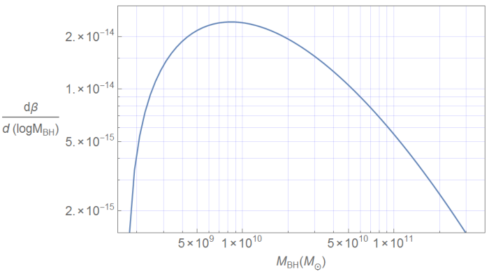
where (18) and (19) have been used to obtain the equality. The mass function for the potential and the inflation-type potential is shown in Figs. 13 and 14. These show that it is indeed possible to choose the model parameters to realize the PBH mass function with the right abundance (see (6)) and at the right mass, here taken to be The width of the mass function turns out to be

References
- [1] SDSS, X. Fan et al., Astron.J. 125, 1649 (2003), astro-ph/0301135.
- [2] C. J. Willott, R. J. McLure, and M. J. Jarvis, Astrophys.J. 587, L15 (2003), astro-ph/0303062.
- [3] J. D. Kurk et al., Astrophys.J. 669, 32 (2007), 0707.1662.
- [4] L. Jiang et al., Astron.J. 134, 1150 (2007), 0707.1663.
- [5] C. J. Willott et al., Astron.J. 134, 2435 (2007), 0706.0914.
- [6] L.-H. Jiang et al., Astron.J. 135, 1057 (2008), 0708.2578.
- [7] L. Jiang et al., Astron.J. 138, 305 (2009), 0905.4126.
- [8] C. J. Willott et al., Astron.J. 139, 906 (2010), 0912.0281.
- [9] C. J. Willott et al., Astron.J. 140, 546 (2010), 1006.1342.
- [10] G. De Rosa et al., Astrophys.J. 739, 56 (2011), 1106.5501.
- [11] D. J. Mortlock et al., Nature 474, 616 (2011), 1106.6088.
- [12] G. De Rosa et al., Astrophys.J. 790, 145 (2014), 1311.3260.
- [13] E. Banados et al., Astron.J. 148, 14 (2014), 1405.3986.
- [14] X.-B. W. et al., Nature 518, 512 (2015).
- [15] V. Dokuchaev, Y. Eroshenko, and S. Rubin, (2007), 0709.0070.
- [16] M. Volonteri, Astron.Astrophys.Rev. 18, 279 (2010), 1003.4404.
- [17] A. Sesana, Adv.Astron. 2012, 805402 (2012), 1110.6445.
- [18] E. Treister and C. M. Urry, Adv.Astron. 2012, 516193 (2012), 1112.0320.
- [19] Z. Haiman, (2012), 1203.6075.
- [20] Y.B.Zel’dovich and I.D.Novikov, Sov.Astron. 10, 602 (1967).
- [21] S. Hawking, Mon.Not.Roy.Astron.Soc. 152, 75 (1971).
- [22] B. J. Carr and S. Hawking, Mon.Not.Roy.Astron.Soc. 168, 399 (1974).
- [23] P. Ivanov, P. Naselsky, and I. Novikov, Phys. Rev. D 50, 7173 (1994).
- [24] J. Garcia-Bellido, A. D. Linde, and D. Wands, Phys.Rev. D54, 6040 (1996), astro-ph/9605094.
- [25] J. Yokoyama, Astron.Astrophys. 318, 673 (1997), astro-ph/9509027.
- [26] M. Kawasaki, N. Sugiyama, and T. Yanagida, Phys.Rev. D57, 6050 (1998), hep-ph/9710259.
- [27] J. Yokoyama, Phys.Rev. D58, 083510 (1998), astro-ph/9802357.
- [28] M. Kawasaki and T. Yanagida, Phys.Rev. D59, 043512 (1999), hep-ph/9807544.
- [29] J. Yokoyama, Phys.Rept. 307, 133 (1998).
- [30] A. Taruya, Phys.Rev. D59, 103505 (1999), hep-ph/9812342.
- [31] T. Kanazawa, M. Kawasaki, and T. Yanagida, Phys.Lett. B482, 174 (2000), hep-ph/0002236.
- [32] T. Kawaguchi, M. Kawasaki, T. Takayama, M. Yamaguchi, and J. Yokoyama, Mon.Not.Roy.Astron.Soc. 388, 1426 (2008), 0711.3886.
- [33] R. Saito, J. Yokoyama, and R. Nagata, JCAP 0806, 024 (2008), 0804.3470.
- [34] L. Alabidi and K. Kohri, Phys.Rev. D80, 063511 (2009), 0906.1398.
- [35] P. H. Frampton, M. Kawasaki, F. Takahashi, and T. T. Yanagida, JCAP 1004, 023 (2010), 1001.2308.
- [36] T. Suyama and J. Yokoyama, Phys.Rev. D84, 083511 (2011), 1106.5983.
- [37] K. Kohri, C.-M. Lin, and T. Matsuda, Phys.Rev. D87, 103527 (2013), 1211.2371.
- [38] M. Kawasaki, A. Kusenko, and T. T. Yanagida, Phys.Lett. B711, 1 (2012), 1202.3848.
- [39] M. Kawasaki, N. Kitajima, and T. T. Yanagida, Phys.Rev. D87, 063519 (2013), 1207.2550.
- [40] T. Suyama, Y.-P. Wu, and J. Yokoyama, Phys.Rev. D90, 043514 (2014), 1406.0249.
- [41] B. J. Carr, J. Gilbert, and J. E. Lidsey, Phys.Rev. D50, 4853 (1994), astro-ph/9405027.
- [42] Planck, P. Ade et al., (2015), 1502.01589.
- [43] Planck, P. Ade et al., (2015), 1502.01592.
- [44] B. J. Carr and J. E. Lidsey, Phys.Rev. D48, 543 (1993).
- [45] J. Chluba, A. L. Erickcek, and I. Ben-Dayan, Astrophys.J. 758, 76 (2012), 1203.2681.
- [46] K. Kohri, T. Nakama, and T. Suyama, Phys.Rev. D90, 083514 (2014), 1405.5999.
- [47] D. Fixsen et al., Astrophys.J. 473, 576 (1996), astro-ph/9605054.
- [48] D. Jeong, J. Pradler, J. Chluba, and M. Kamionkowski, Phys.Rev.Lett. 113, 061301 (2014), 1403.3697.
- [49] T. Nakama, T. Suyama, and J. Yokoyama, Phys.Rev.Lett. 113, 061302 (2014), 1403.5407.
- [50] A. A. Starobinsky, JETP Lett. 42, 152 (1985).
- [51] D. Salopek and J. Bond, Phys.Rev. D42, 3936 (1990).
- [52] M. Sasaki and E. D. Stewart, Prog.Theor.Phys. 95, 71 (1996), astro-ph/9507001.
- [53] M. Sasaki and T. Tanaka, Prog.Theor.Phys. 99, 763 (1998), gr-qc/9801017.
- [54] D. Wands, K. A. Malik, D. H. Lyth, and A. R. Liddle, Phys.Rev. D62, 043527 (2000), astro-ph/0003278.
- [55] D. H. Lyth, K. A. Malik, and M. Sasaki, JCAP 0505, 004 (2005), astro-ph/0411220.
- [56] M. Shibata and M. Sasaki, Phys.Rev. D60, 084002 (1999), gr-qc/9905064.
- [57] J. C. Niemeyer and K. Jedamzik, Phys.Rev. D59, 124013 (1999), astro-ph/9901292.
- [58] I. Hawke and J. Stewart, Class.Quant.Grav. 19, 3687 (2002).
- [59] A. G. Polnarev and I. Musco, Class.Quant.Grav. 24, 1405 (2007), gr-qc/0605122.
- [60] A. Polnarev, T. Nakama, and J. Yokoyama, JCAP 1209, 027 (2012), 1204.6601.
- [61] T. Harada, C.-M. Yoo, and K. Kohri, Phys.Rev. D88, 084051 (2013), 1309.4201.
- [62] T. Nakama, T. Harada, A. Polnarev, and J. Yokoyama, JCAP 1401, 037 (2014), 1310.3007.
- [63] T. Nakama, JCAP 1410, 040 (2014), 1408.0955.
- [64] T. Harada, C.-M. Yoo, T. Nakama, and Y. Koga, Phys.Rev. D91, 084057 (2015), 1503.03934.
- [65] A. A. Starobinsky, Lect.Notes Phys. 246, 107 (1986).
- [66] A. A. Starobinsky, Phys. Lett. B117, 175 (1982).
- [67] D. Lyth and A. Liddle, Cambridge University Press (2009).
- [68] Planck, P. Ade et al., (2015), 1502.02114.
- [69] K.-i. Maeda, Phys. Rev. D37, 858 (1988).
- [70] A. A. Starobinsky, Phys.Lett. B91, 99 (1980).
- [71] N. Takeda and Y. Watanabe, Phys.Rev. D90, 023519 (2014), 1405.3830.