Optimal ALOHA-like Random Access with Heterogeneous QoS Guarantees for Multi-Packet Reception Aided Visible Light Communications

Let $R_{j}(t)$ denote the instantaneously achievable transmission rate of the device $j$ at the time slot $t$, $j=1,\cdots,N$. The fundamental part of modelling EC of the device $j$ is to find the probability distribution of $R_{j}(t)$. $R_{j}(t)$ and its probability distribution are influenced by the MIMO-SIC algorithm and the ALOHA-like random access algorithm that is characterised by the access probability vector p. To emphasize the effect of p on EC, we define $\mathsf{EC}_{j}(\textbf{p};\theta_{j})$ as the EC of device $j$ in the remainder part. It is extremely difficult to quantify the impact of the MIMO-SIC algorithm on $R_{j}(t)$ because of the randomness of the interference relations existing among the links.

For solving the above EC derivation problem, we model the ALOHA-like random access aided VLC network as a conflict graph $\cal G=(\cal{V},\cal{E})$, where $\cal V$ denotes the set of devices, $\cal E$ denotes the set of interference relations among links. There is an edge between two vertices in $\cal G$ if their links interfere with each other. The vector $\bm{\sigma}^{i}\in{\{{0,1}\}}^{N}$ is defined as the state $i$ of $\cal G$, $i=1,\cdots,2^{N}$, and $\sigma_{j}^{i}$ denotes the $j$-th element in $\bm{\sigma}^{i}$, $j=1,\cdots,N$. $\sigma_{j}^{i}=1$ represents that the device $j$ transmits signals to the coordinator and it is non-blocked in the state $\bm{\sigma}^{i}$; otherwise, we have $\sigma_{j}^{i}=0$. For example, the current state of $\cal G$ corresponding to the system of Fig. 1 is $[1,0,1,0,1]$⁴⁴ 4 In the random access VLC system considered, not all of the devices transmit data packets to the coordinator in each time slot. In the particular time slot shown in Fig. 1, the device $2$ does not transmit data packets, thus the second element of the vector characterizing the current state of $\cal G$ is $0$.. Since the device $j$ does not know if it is blocked before its transmission, we obtain:

where $p_{j}$ denotes the access probability of the device $j$. Note that $\sigma^{i}_{j}=1$ does not mean that the transmission of the device $j$ is successful because collisions might happen.

Because we adopt the slotted ALOHA-like random access mechanism, the states of $\cal G$ in different time slots are independent and identically distributed. The probability of the occurrence of the state $\bm{\sigma}^{i}$, defined as $\pi({\boldsymbol{\sigma}^{i}})$, is given by

Note that herein $\pi$ is the steady state distribution probability rather than the mathematical constant that represents the ratio of a circle’s circumference to its diameter.

$\cal I$ is defined as the set of the feasible access states of $\cal G$, and ${\cal I}={\{{\boldsymbol{\sigma}^{i}:\tau_{i}\leq M}\}}$.

In this paper, we adopt the MIMO-SIC algorithm to achieve MPR for the coordinator⁵⁵ 5 In random access systems, the group of concurrently transmitting devices is random, and the coordinator does not even know the number of these devices, which imposes challenges on the channel estimation. As a result, the implementation and performance analysis of the MIMO-SIC algorithm are affected. In fact, the number of simultaneously transmitting devices can be estimated by using the threshold based rank estimation algorithm, and then existing MIMO channel estimation algorithms can be used.. That is, after the signal of one device is decoded, its signal is stripped away from the aggregate received signal before the signal of the next device is decoded [13, 28]. We assume that no device is decoded successfully in the infeasible access state, while in the feasible access state $\bm{\sigma}^{i}$ we assume the SIC procedure of the MIMO-SIC algorithm is ideal, i.e., there is no error propagation in the decoding process. The performance of the MIMO-SIC algorithm is dependant on the detection ordering method, which is represented by a $\tau_{i}\times\tau_{i}$ matrix $\bf{F}$. If and only if the signal of the device $j$ is decoded at the $l$-th layer, we have $F_{jl}=1$. Otherwise, we have $F_{jl}=0$. After using the detection ordering, the rearranged channel matrix and the transmitted signal are denoted as $\bf{\tilde{H}}$ and $\tilde{\bf{x}}$, which are given by $\tilde{\bf{H}}=\bf{H}\bf{F}$ and $\tilde{\bf{x}}=\bf{F}\bf{x}$, respectively. The LOS channel gain vector of the device $j$ is defined as ${\bf{h}}_{j}$ that is the $j$-th column of $\bf{H}$. The LOS channel gain vector of the device decoded at the $k$-th layer is defined as $\tilde{\bf{h}}_{k}$ that is the $k$-th column of $\bf{\tilde{H}}$. Additionally, $x_{j}$ is the transmitted signal of the device $j$, and $\tilde{x}_{k}$ is the signal decoded at the $k$-th layer. After decoding and removing $l-1$ signals, the residual received signal vector is given by ${\bf{r}}_{l}=\sum\limits_{k=l}^{\tau_{i}}\xi P_{\text{t}}\tilde{\bf{h}}_{k}\tilde{x}_{k}+{\bf{v}}$. If $F_{jl}=1$, we have ${\tilde{\bf{h}}}_{l}={\bf{h}}_{j}$ and ${\tilde{\bf{x}}}_{l}={\bf{x}}_{j}$, then

Let ${\bf{z}}_{l}$ denote the output of the MIMO detector (e.g. ZF or minimum mean-squared error (MMSE) filter) at the $l$-th layer. ${\bf{W}}^{l}$ is defined as the filter matrix used at the $l$-th layer, and ${\bf{W}}^{l}_{j}$ denotes the $j$-th row in ${\bf{W}}^{l}$ [13]. At the $l$-th layer, the channel gains of the residual devices are organized into the residual channel matrix ${\bf{\tilde{H}}}_{l}=[\tilde{\bf{h}}_{l},\cdots,\tilde{\bf{h}}_{\tau_{i}}]$. The $j$-th element of ${\bf z}_{l}$ is given by

Hence, the signal-to-interference-plus-noise ratio (SINR) of the device $j$ in the feasible access state $\bm{\sigma}^{i}$ is:

If the ZF filter [13, 28] is used, ${\bf{W}}^{l}_{j}$ is the $j$-th row of the matrix ${\left({{\bf{\tilde{H}}}_{l}}^{H}{\bf{\tilde{H}}}_{l}\right)}^{-1}{\bf{\tilde{H}}}_{l}^{H}$, and the SINR of the device $j$ in the feasible access state $\bm{\sigma}^{i}$ is:

If the MMSE filter [13, 28] is used,

and the SINR of the device $j$ in the feasible access state $\bm{\sigma}^{i}$ is given by

Using Shannon’s capacity formula, the upper bound on the instantaneously achievable transmission rate [bits/s] of the device $j$ in the feasible access state ${\boldsymbol{\sigma}^{i}}$ is given by

The instantaneously achievable transmission rate of the device $j$ only depends on the state of $\cal{G}$ (i.e., the set of the devices that are simultaneously transmitting signals) and their corresponding channel gains. The individual channel gains of these devices can be regarded as fixed provided that these devices are unblocked and their positions are unchanged. Because the states of $\cal{G}$ in different time slots are independent and identically distributed, the instantaneously achievable transmission rates of the device $j$ are independent and identically distributed across different time slots. The probability of $\left\{R_{j}(t)=R_{j}^{i}\right\}$ equals the probability of the occurrence of the feasible access state $\bm{\sigma}^{i}$ that satisfies $\sigma_{j}^{i}=1$, and is given by

where ${\cal{I}}_{j}$ is defined as the set of the feasible access states satisfying that the device $j$ is transmitting signals to the coordinator and is unblocked, ${\cal{I}}_{j}={\{{\boldsymbol{\sigma}^{i}:\tau_{i}\leq M,\sigma_{j}^{i}=1}\}}$. Furthermore, the probability of $\left\{R_{j}(t)=0\right\}$ equals the probability of all events that the device $j$ transmits unsuccessfully, which is given by

Accordingly, the EC of the device $j$ is formulated as (21).

Saturation throughput refers to the network throughput when devices always have data to transmit [19]. According to (19), the saturation throughput is formulated as

In this paper, we aim to find the optimum access probability vector ${\textbf{p}}=[p_{1},\cdots,p_{N}]$ so that the saturation throughput is maximized for the VLC system subject to the heterogeneous delay QoS constraints. For a given QoS exponent vector $\boldsymbol{\theta}=\left[{\theta_{1},\cdots,\theta_{N}}\right]$, the optimization problem (OP) is formulated as

where $\mathsf{EB}_{j}(\theta_{j})$ denotes the EB [21] of the traffic of the device $j$, given by

in which $A_{j}(t)$ denotes the accumulated arrival process of the device $j$ over the time interval $[0,t)$. $\mathsf{EC}_{j}({\textbf{p}};\theta_{j})\geq\mathsf{EB}_{j}(\theta_{j})$ represents that the QoS constraint of device $j$ has to be satisfied [23]. $0<{p_{j}}\leq 1$ represents that the access probability of device $j$ must range from $0$ to $1$. $\theta_{j}=0$ denotes that the device $j$ has no QoS requirement.

The classical IWO algorithm [29] cannot handle the COP directly, thus we transform the single-objective COP (24) into a bi-objective unconstrained OP (a special case of MOP, which is also called vector optimization problems [31]). We employ the modified IWO algorithm relying on Pareto optimization technologies to cope with the bi-objective OP. Referring to [30], the unconstrained bi-objective OP is given as the element-wise minimization problem of

where the first objective $\displaystyle\frac{1}{\eta({\textbf{p}})}$ is the original objective in the OP (24), and the second objective $\Omega({\textbf{p}})$ is the sum of all constraint violations in the OP (24). More specifically, $\Omega({\textbf{p}})$ is defined as follows:

Obviously, we have $\Omega({\textbf{p}})\geq 0$, and all the constraints in (24) are satisfied if and only if $\Omega({\textbf{p}})=0$.

The optimization variable p of the problem (25), i.e. the access probability vector in this paper, is taken as the position of the weed in the search space. The number of devices in the VLC system is $N$, hence p is an $N$-dimensional variable. As a result, the search space of our IWO-DE algorithm is $N$-dimensional. Without causing confusion, in what follows both the position of the weed and the weed itself may represent the access probability vector. The candidate access probability vector that has smaller fitness value, as define in (30), is closer to the optimum access probability vector and thus more likely to reproduce and survive. For simultaneously achieving minimization of the two objectives in (25), some modifications are made in the reproduction step and the competitive exclusion step of the IWO algorithm. The key steps of the modified IWO algorithm are presented as follows.

Step 1) Initialization: A number of initial candidate solutions defined as ${\cal P}=\{{{\textbf{p}}}^{i},i=1,\cdots,W_{0}\}$ are randomly dispersed over the $N$-dimension space. $W_{0}$ denotes the number of the initial candidate solutions. ${\textbf{p}}^{i}$ is the $i$-th weed, i.e., the $i$-th candidate solution of the problem (25), in the population, and it is an $1\times N$ vector with element $p_{j}^{i}$ representing the access probability of the device $j$.

Step 2) Reproduction: To accommodate IWO for the MOP, we adopt the adaptive weighted sum fitness assignment mechanism [30] to determine the number of the offspring reproduced by each weed. For the weed $\textbf{p}^{i}$, the fitness value of ${{\textbf{p}}^{i}}$, denoted as ${fit({{\textbf{p}}^{i}})}$, is defined as follows:

where

in which we have $\displaystyle f({\textbf{p}}^{i})=\frac{1}{\eta({\textbf{p}}^{i})}$ and $W=W_{0}$ if $Z=0$. Otherwise, $W=W_{\max}$. $Z$ denotes the iteration index, and also denotes the generation index. $W_{\max}$ denotes the maximum number of survival weeds.

Hence, the number of offspring reproduced by the $i$-th weed ${{\textbf{p}}^{i}}$ is formulated as follows [29]:

where $S_{\max}$ denotes the permissible maximum number of offspring, and $S_{\min}$ denotes the permissible minimum number of offspring.

Step 3) Spatial Dispersion: The generated offspring of the $i$-th weed ${\textbf{p}}^{i}$ are randomly dispersed over the search space. The offspring obey the normal distribution with varying standard deviations. The mean of the normal distribution is zero, and its standard deviation gradually reduces from an initial value $\sigma_{\text{initial}}$ to a final value $\sigma_{\text{final}}$ in each generation. The standard deviation at each iteration is expressed as [29]:

where $Z_{\max}$ is the maximum number of iterations, $\sigma_{Z}$ is the standard deviation in the $Z$-th iteration and ${\phi}$ is the non-linear modulation index⁶⁶ 6 In the IWO algorithm, the non-linear modulation index ${\phi}$ is a terminology that determines the variation degree of the offspring. of the IWO algorithm [29].

Step 4) Competitive Exclusion: In order to limit the number of the weeds that serve as inputs to the DE procedure, weeds and their offspring are ranked together to eliminate weeds that have poor (i.e. high herein) fitnesses values in this step. More specifically, to minimize the two objectives in (25) simultaneously, we adopt the non-dominated sorting [30] to decide which individual to survive into the next generation. The non-dominated sorting is based on Pareto dominance [30], which ensures that the candidate solutions obtained in the IWO procedure distribute surrounding the Pareto front [30]. As a beneficial result, the convergence of the algorithm is accelerated. The definition of Pareto dominance is given as follows [30]:

Accordingly, the exclusion mechanism of IWO is as follows:

• •

  if the weed ${{\textbf{p}}}^{i}$ Pareto-dominates the weed ${{\textbf{p}}}^{j}$, the weed ${{\textbf{p}}}^{i}$ wins;

• •

  otherwise, the weed with smaller sum constraint violation value $\Omega(\textbf{p})$ wins.

The top $W_{\max}$ weeds are taken as the optimum candidates used as the inputs of the DE procedure. Having carried out the refinement procedures of IWO, the excellent weeds are picked out. Then, the DE algorithm is applied with respect to the selected weeds, which essentially explores the search space to obtain the optimum solution.

The variation of the DE procedure is created to find the global optimum solution by means of three operations, i.e., mutation, crossover and selection [30].

Step 1) Mutation Operation: In the mutation operation, a mutant vector ${\bm{\alpha}^{i}}$ is built as follows [30]:

where ${\textbf{p}^{\text{best}}}$ denotes the best weed obtained in the IWO procedure, $r_{1}$ and $r_{2}$ denote randomly selected indices, $\textbf{p}^{r_{1}}$ denotes the $r_{1}$-th weed in the IWO procedure, and $\textbf{p}^{r_{2}}$ denotes the $r_{2}$-th weed in the IWO procedure. $F_{0}$ is a scaling factor that quantifies the difference between $\textbf{p}^{r_{1}}$ and $\textbf{p}^{r_{2}}$. Each weed in the IWO procedure corresponds to a mutant vector in the DE procedure. $\bm{\alpha}^{i}$ is a $1\times N$ vector, $i=1,\cdots,W_{\max}$.

Step 2) Crossover Operation: With the mutant vector $\bm{\alpha}^{i}$ and the vector $\textbf{p}^{i}$, another trial vector $\textbf{u}^{i}$ is generated through the binomial crossover as follows [30]:

where $i=1,\cdots,W_{\max}$, $j=1,\cdots,N$, $j_{\text{rand}}$ is a randomly selected integer ranging from $1$ to $N$, which ensures $\textbf{u}^{i}$ inherits at least one component from the mutant vector $\bm{\alpha}^{i}$. Additionally, $\text{rand}_{j}$ is a r.v. obeying the uniform distribution and $0\leq\text{rand}_{j}\leq 1$. $C_{\text{r}}$ is the crossover probability. $\alpha_{j}^{i}$, $p_{j}^{i}$ and $u_{j}^{i}$ denote the $j$-th element in $\bm{\alpha}^{i}$, $\textbf{p}^{i}$ and $\textbf{u}^{i}$, respectively.

Step 3) Selection Operation: $\textbf{u}^{i}$ is chosen as the replacements of $\textbf{p}^{i}$ in the next generation only when ${\textbf{u}}^{i}$ leads to a better solution. Hence, the selection operation is described by:

For the sake of clarity, the whole framework of IWO-DE is presented in Table I. The search space of our IWO-DE is $N$-dimensional. Hence, the computational complexity of the IWO-DE algorithm is ${\cal{O}}\left[Z_{\max}W_{\max}S_{\max}(N+W_{\max}S_{\max})\right]$. A larger maximum number of weeds ($W_{\max}$) and a higher maximum number of offspring ($S_{\max}$) may improve the quality of the optimum access probability vector obtained, while imposing an increased computational complexity.

To sum up, our QoS-guaranteed ALOHA-like random access algorithm relies on the IWO-DE algorithm to find the optimal access probability for each device. Each device transmits its traffic information containing the traffic type (determined by the statistical property of the traffic) and the QoS requirement to the coordinator. The coordinator calculates devices’ optimal access probabilities by solving the OP (24) with the help of the IWO-DE algorithm⁷⁷ 7 The coordinator does not need to recalculate the devices’ optimal access probabilities provided that the individual channel gains and traffic information (i.e., the traffic type and QoS requirement) of these devices are unchanged. In this case, the IWO-DE is an off-line optimization algorithm for the problem considered. Hence, it does not make sense to incorporate the processing time of the IWO-DE algorithm into the statistical transmission delay considered, which is related with the underlying buffer size and the arrival information rate.. Then, the coordinator broadcasts the optimum access probability vector for devices in the beacon frame. Finally, each device distributedly transmits its respective data to the coordinator with its unique optimum access probability.

Our Monte Carlo simulation is based on $5\times 10^{5}$ times repeated trials⁸⁸ 8 An ALOHA-like random access VLC system was simulated, where the individual instantaneous service rates of $5\times 10^{5}$ time slots were recorded for evaluating the EC according to (8).. Table III shows the theoretical EC results and the Monte Carlo simulation results in the situation that all devices randomly pick their probabilities of being unblocked, access probabilities and QoS exponents. It is demonstrated that our analytical EC expression of (21) matches accurately with the results of the Monte Carlo simulation.

Fig. 2 shows the EC comparison results when the coordinator has different MPR capabilities, indicated by $M$. It is demonstrated that the EC grows with the increase of the MPR capability $M$ of the coordinator. Fig. 2 also indicates the accuracy of our analytical EC expression of (21). Additionally, it demonstrates that the EC decreases with the increase of the QoS exponent. The reason is that higher QoS exponent indicates more stringent delay QoS requirement. For a given service process, the maximum constant arrival rate that can be supported will decrease under stricter delay QoS requirement.

Fig. 3 and Fig. 4 depict the maximum saturation throughput and the percentage of the feasible solutions of the IWO-DE algorithm with respect to different values of the maximum weed size $W_{\max}$ in the random situation, where the devices randomly pick their blocking status and the traffic parameters, such as the probability of being unblocked ranging from $0.7$ to $1$, the arrival parameters ranging from $0.001$ to $0.01$, the QoS exponent ranging from $10^{-10}$ to $10^{-6}$. Obviously, increasing the maximum weed size from 20 to 80 improves the performance of the IWO-DE algorithm after convergence. Fig. 3 shows that the IWO-DE search algorithm is trapped into the local optimal solution when $W_{\max}=20$. This is because DE is a population-based method. The small maximum weed size $W_{\max}$ limits the variation of the DE procedure, and then limits the global search ability of the DE method. In Fig. 4, the curve of $W_{\max}=20$ is steeper than the others. The reason is that the population size of $W_{\max}=20$ is much lower than the other two situations. Fig. 3 and Fig. 4 indicate that our IWO-DE algorithm has a desirable convergence when $W_{\max}=50$. Considering the convergence as well as the computational complexity, we choose $W_{\max}=50$ as the specific value used in the following simulations.

Fig. 5 shows the comparison of the saturation throughput achieved by our QoS-guaranteed ALOHA-like random access algorithm and by the CSMA/CA algorithm of the IEEE 802.15.7 standard [6, 32]. In Scenario 1 and Scenario 2, the difference in the channel gains of the devices is assumed to be large and small⁹⁹ 9 To achieve this “channel-gain difference” goal in a fair manner for both algorithms, the actual locations of the devices are particularly selected from a larger set of uniformly distributed positions in both Scenario 1 and Scenario 2. More specifically, considering the benchmark single-packet reception, i.e., $M=1$, we first calculate the individual instantaneous PHY transmission rates for all the elements of the larger position set, and then select two identical-size subsets of positions so that the channel-gain difference of one subset is large and the other is small, while making sure the average PHY transmission rate of both subsets is the same. As a result, all the devices share a common access probability of $p=1/N$ and for the CSMA/CA algorithm, the saturation throughput is equal in both scenarios, since it is insensitive to the channel-gain difference, as demonstrated by the results of Fig. 5., respectively. In both scenarios, none of the devices is blocked, i.e., the channels are assumed to be ideal. Additionally, we assume that all the devices share the common QoS exponent constraint $\theta=10^{-8}$ and the common arrival parameter $\lambda=0.01$. Referring to [7], we set the parameters of the CSMA/CA algorithm of the IEEE 802.15.7 standard as follows: $macMinBE=3$, $macMaxBE=5$, $macMaxFrameRetries=3$ and $macMaxCSMABackoffs=4$. Furthermore, to make fair comparison, we also utilize Shannon’s capacity formula to calculate the upper bound on the instantaneously achievable PHY transmission rate when quantifying the saturation throughput achieved by the CSMA/CA algorithm of the IEEE 802.15.7 standard.

As observed from Fig. 5, the saturation throughput of our algorithm is far superior to that of the CSMA/CA algorithm, especially in Scenario 1, although the CSMA/CA algorithm benefits from the carrier sensing, which is assumed to be perfect in our simulations. This is because the MPR capability of the proposed algorithm reduces the chance of collisions in the random access procedure. More specifically, our algorithm adaptively adjusts the access probability vector of devices in order to fully utilize the MPR capability. Furthermore, there is no constraint on the minimum service rate of each device in our algorithm. As a result, the devices with higher channel gains have larger access probabilities in the context where they share a common delay QoS exponent value. In other words, the devices with higher channel gains have more chances to transmit data packets to the coordinator and thus a maximized saturation throughput of the VLC system is achieved. Additionally, in our scheme the MPR capability of the coordinator is achieved by using the SIC algorithm, which performs better when there is a substantial difference in the channel gains of the simultaneously transmitting devices, provided that no power control is used [13]. Therefore, the gap of the saturation throughput between our algorithm and the benchmark CSMA/CA algorithm is much larger in Scenario 1 than in Scenario 2. It is worth noting that our algorithm achieves the maximized saturation throughput of the VLC system by sacrificing the fairness, while the benchmark CSMA/CA algorithm guarantees that all devices have equal opportunities to transmit to the coordinator, thus achieving better fairness. We also observe from Fig. 5 that the saturation throughput of both algorithms declines when the number of devices is increased. Nonetheless, the proposed algorithm remains substantially superior to the benchmark CSMA/CA algorithm in term of the saturation throughput achieved. Finally, our algorithm guarantees the statistical delay QoS requirements of devices, hence a marginal decrease in the saturation throughput with the increasing of the number of devices can be regarded as a reasonable cost for obtaining this benefit.

In the scenario of Fig. 6, all the devices share the common QoS constraint $\theta$ and the common probability of being unblocked $\beta$. Additionally, they share the common arrival parameter $\lambda=0.01$. Fig. 6 shows the maximum saturation throughput of our proposed ALOHA-like random access algorithm in different blocking situations. When the MPR capability is smaller, i.e., $M=2$, heavy collisions happens, the achievable maximum throughput of $\beta=0.7$ approaches that of $\beta=0.9$. Whereas the gap between the curve of $\beta=0.7$ and the curve of $\beta=0.9$ increases when $M=4$. This is because the stronger MPR capability alleviates collisions of the VLC system in a greater degree. In such a situation, the benefit of the less severely blocked channel condition becomes prominent. Fig. 6 also shows that the maximum saturation throughput only slightly decreases with the increase of the QoS exponent for the given $M$, which indicates that our QoS-guaranteed ALOHA-like random access algorithm is reliable when the QoS constraint varies.

In the context of Fig. 7 and Fig. 8, the devices are divided into two groups, where $\displaystyle\frac{M}{2}$ devices with the stricter QoS constraint $\theta_{s}$ are in one of the groups, while the remaining devices with $\theta_{l}=10^{-10}$ in the other group. ${\text{S}(2k-1)}$ ($k=1,\cdots,5$) represents the situation of $\theta_{s}=10^{k-11}$ and ${\text{S}(2k)}$ ($k=1,\cdots,4$) represents the situation of $\theta_{s}=5\times 10^{k-11}$. Additionally, they share the common arrival parameter $\lambda=0.01$. Fig. 7 shows the maximum saturation throughput of our QoS-guaranteed ALOHA-like random access algorithm versus $\theta_{s}$. It is demonstrated that the performance of our QoS-guaranteed ALOHA-like random access algorithm remains favourable even when the QoS constraints become stricter, i.e. when $\theta_{s}$ becomes larger. Additionally, the maximum saturation throughput is doubled when the MPR capability $M$ increases from $2$ to $4$, which indicates that our algorithm fully utilizes the MPR capability to improve the performance of the system considered. Fig. 8 shows the value of the generation number $Z$ versus $\theta_{s}$ when all candidate solutions of the IWO-DE algorithm start to be feasible. The fluctuations in Fig. 8 are caused by the randomness inherent in the IWO-DE algorithm, such as the randomly generated offspring in the spatial dispersion step and the random variations in the DE procedure. Obviously, it is harder to search for the feasible access probability vector when $M=2$, which matches the fact that it is harder to guarantee the QoS when the MPR capability $M$ is lower.

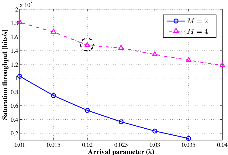
In the scenario of Fig. 9, all devices share the common probability of being unblocked, i.e., $\beta=0.9$. Again, the devices are divided into two groups, where $\displaystyle\frac{M}{2}$ of them with the stricter QoS constraint $\theta_{s}=10^{-7}$ are in one of the groups, while the remaining devices with looser QoS constraint $\theta_{l}=10^{-10}$ in the other group. Fig. 9 shows the maximum saturation throughput of our proposed ALOHA-like random access algorithm versus the common arrival parameter $\lambda$. The maximum saturation throughput declines with the increase of $\lambda$ in the situation that $M=2$, so does in the situation that $M=4$. But the curve of $M=4$ falls more slowly, especially after the noted point. The increase of $\lambda$ makes it more difficult to satisfy the first constraint of the OP (24). Thus the set of the feasible solutions of (24) becomes smaller. As a result, the achievable maximum saturation throughput becomes lower. Furthermore, there is no feasible solution to the OP (24) when $M=2$ and $\lambda=0.04$. In other words, the QoS requirement cannot be guaranteed in this situation. Furthermore, after the noted point in Fig. 9 the maximum saturation throughput of $M=4$ is more than twice that of $M=2$. It is demonstrated that increasing the MPR capability of the coordinator obtains remarkable performance advantage when $\lambda$ is larger.

References

- [1] S. Wu, H. Wang, and C. Youn, “Visible light communications for 5G wireless networking systems: From fixed to mobile communications,” IEEE Netw., vol. 28, no. 6, pp. 41–45, Nov./Dec. 2014.
- [2] M. Chen, J. Wan, S. Gonzalez, X. Liao, and V. Leung, “A survey of recent developments in home M2M networks,” IEEE Commun. Surveys Tuts., vol. 16, no. 1, pp. 98–114, 1st Quart. 2014.
- [3] M. Agiwal, A. Roy, and N. Saxena, “Next generation 5G wireless networks: A comprehensive survey,” IEEE Commun. Surveys Tuts., vol. PP, no. 99, pp. 1–1, 2016.
- [4] Y. Liu, C. Yeh, C. Chow, Y. Liu, Y. Liu, and H. Tsang, “Demonstration of bi-directional LED visible light communication using TDD traffic with mitigation of reflection interference,” Opt. Express, vol. 20, no. 21, pp. 23 019–23 024, Oct. 2012.
- [5] Y. Wang, N. Chi, Y. Wang, L. Tao, and J. Shi, “Network architecture of a high-speed visible light communication local area network,” IEEE Photon. Technol. Lett., vol. 27, no. 2, pp. 197–200, Jan. 2015.
- [6] IEEE Standard for Local and Metropolitan Area Networks–Part 15.7: Short-Range Wireless Optical Communication Using Visible Light, IEEE Std. 802.15.7-2011, Sep. 2011.
- [7] S. Nobar, K. Mehr, and J. Niya, “Comprehensive performance analysis of IEEE 802.15.7 CSMA/CA mechanism for saturated traffic,” J. Opt. Commun. Netw., vol. 7, no. 2, pp. 62–73, Feb. 2015.
- [8] Q. Wang and D. Giustiniano, “Intra-frame bidirectional transmission in networks of visible LEDs,” IEEE/ACM Trans. Netw., 2016 (early access in IEEE Xplore).
- [9] O. Ergul, E. Dinc, and O. Akan, “Communicate to illuminate: State-of-the-art and research challenges for visible light communications,” Phys. Commun., vol. 17, pp. 72–85, Dec. 2015.
- [10] T. Komine and M. Nakagawa, “Fundamental analysis for visible-light communication system using LED lights,” IEEE Trans. Consum. Electron., vol. 50, no. 1, pp. 100–107, Feb. 2004.
- [11] M. Biagi, S. Pergoloni, and A. Vegni, “LAST: A framework to localize, access, schedule, and transmit in indoor VLC systems,” J. Lightw. Technol., vol. 33, no. 9, pp. 1872–1887, May 2015.
- [12] D. Chan, T. Berger, and L. Tong, “Carrier sense multiple access communications on multipacket reception channels: Theory and applications to IEEE 802.11 wireless networks,” IEEE Trans. Commun., vol. 61, no. 1, pp. 266–278, Jan. 2013.
- [13] S. Yang and L. Hanzo, “Fifty years of MIMO detection: The road to large-scale MIMOs,” IEEE Commun. Surveys Tuts., vol. 17, no. 4, pp. 1941–1988, 4th Quart. 2015.
- [14] L. Zhao, X. Chi, P. Li, and L. Guan, “A MPR optimization algorithm for FSO communication system with star topology,” Opt. Commun., vol. 356, pp. 147–154, Dec. 2015.
- [15] S. Gollakota and D. Katabi, “ZigZag decoding: Combating hidden terminals in wireless networks,” ACM SIGCOMM Computer Communication Review, vol. 38, no. 4, pp. 159–170, Aug. 2008.
- [16] Y. Zhang, P. Zheng, and S. Liew, “How does multiple-packet reception capability scale the performance of wireless local area networks?” IEEE Trans. Mobile Comput., vol. 8, no. 7, pp. 923–935, Jul. 2009.
- [17] Y. Zhang, “Multi-round contention in wireless LANs with multipacket reception,” IEEE Trans. Wireless Commun., vol. 9, no. 4, pp. 1503–1513, Apr. 2010.
- [18] Y. Bae, B. Choi, and A. Alfa, “Achieving maximum throughput in random access protocols with multipacket reception,” IEEE Trans. Mobile Comput., vol. 13, no. 3, pp. 497–511, Mar. 2014.
- [19] S. Wu, W. Mao, and X. Wang, “Performance study on a CSMA/CA-based MAC protocol for multi-user MIMO wireless LANs,” IEEE Trans. Wireless Commun., vol. 13, no. 6, pp. 3153–3166, Jun. 2014.
- [20] H. Yu, X. Chi, and J. Liu, “An integrated PHY-MAC analytical model for IEEE 802.15.7 VLC network with MPR capability,” Opt. Lett., vol. 10, no. 5, pp. 365–368, Sep. 2014.
- [21] C. Chang and J. Thomas, “Effective bandwidth in high-speed digital networks,” IEEE J. Sel. Areas Commun., vol. 13, no. 6, pp. 1091–1100, Aug. 1995.
- [22] D. Wu and R. Negi, “Effective capacity: A wireless link model for support of quality of service,” IEEE Trans. Wireless Commun., vol. 2, no. 4, pp. 630–644, Jul. 2003.
- [23] A. Aijaz, M. Tshangini, M. Nakhai, X. Chu, and A. Aghvami, “Energy-efficient uplink resource allocation in LTE networks with M2M/H2H co-existence under statistical QoS guarantees,” IEEE Trans. Commun., vol. 62, no. 7, pp. 2353–2365, Jul. 2014.
- [24] Y. Li, L. Liu, H. Li, J. Zhang, and Y. Yi, “Resource allocation for delay-sensitive traffic over LTE-advanced relay networks,” IEEE Trans. Wireless Commun., vol. 14, no. 8, pp. 4291–4303, Aug. 2015.
- [25] F. Jin, R. Zhang, and L. Hanzo, “Resource allocation under delay-guarantee constraints for heterogeneous visible-light and RF femtocell,” IEEE Trans. Wireless Commun., vol. 14, no. 2, pp. 1020–1034, Feb. 2015.
- [26] S. Efazati and P. Azmi, “Statistical quality of service provisioning in multi-user centralised networks,” IET. Commun., vol. 9, no. 5, pp. 621–629, Mar. 2015.
- [27] R. Smith and S. Personick, “Receiver design for optical fiber communication systems,” in Semiconductor Devices for Optical Communication, H. Kressel, Ed. New York: Springer-Verlag, 1980.
- [28] D. Tse and P. Viswanath, Fundamentals of Wireless Communication. New York, USA: Cambridge University Press, 2005.
- [29] A. Mehrabian and C. Lucas, “A novel numerical optimization algorithm inspired from weed colonization,” Ecol. Inform., vol. 1, no. 4, pp. 355–366, Dec. 2006.
- [30] X. Cai, Z. Hu, and Z. Fan, “A novel memetic algorithm based on invasive weed optimization and differential evolution for constrained optimization,” Soft Computing, vol. 17, no. 10, pp. 1893–1910, Oct. 2013.
- [31] S. Boyd and L. Vandenberghe, Convex Optimization. New York, USA: Cambridge University Press, 2004.
- [32] P. Pathak, X. Feng, P. Hu, and P. Mohapatra, “Visible light communication, networking, and sensing: A survey, potential and challenges,” IEEE Commun. Surveys Tuts., vol. 17, no. 4, pp. 2047–2077, 4th Quart. 2015.
![[Uncaptioned image]](1609.02227v1/Linlin.png) |
Linlin Zhao received her B.Eng. and M.S. degrees from the Department of Communication Engineering, Jilin University, Changchun, China in 2009 and 2012, respectively. She is currently pursuing the Ph.D. degree in the Department of Communication Engineering, Jilin University, Changchun, China. Her research interests include the throughput optimal random access algorithms, resource allocation schemes, delay analysis and optimization in random access aided wireless networks. |
![[Uncaptioned image]](1609.02227v1/chi2.png) |
Xuefen Chi received her B.Eng. degree in Information Engineering from Beijing University of Posts and Telecommunications (BUPT), Beijing, China in Jul. 1984. She received the M.S. and Ph.D. degree from Changchun Institute of Optics, Fine Mechanics and Physics, Chinese Academy of Sciences, Changchun, China, in 1990 and 2003 respectively. She was a visiting scholar at Department of Computer Science, Loughborough University, England, UK, in 2007, and School of Electronics and Computer Science, University of Southampton, Southampton, UK, in 2015. Currently, she is a professor at the Department of Communication Engineering, Jilin University, China. Her research interests include machine type communication, indoor visible light communication, random access algorithms, delay-QoS guarantees, queuing theory and its applications. |
![[Uncaptioned image]](1609.02227v1/Shaoshi.png) |
Shaoshi Yang received his B.Eng. degree in Information Engineering from Beijing University of Posts and Telecommunications (BUPT), Beijing, China in Jul. 2006, his first Ph.D. degree in Electronics and Electrical Engineering from University of Southampton, U.K. in Dec. 2013, and his second Ph.D. degree in Signal and Information Processing from BUPT in Mar. 2014. He is now working as a Postdoctoral Research Fellow in University of Southampton, U.K. From November 2008 to February 2009, he was an Intern Research Fellow with the Communications Technology Lab (CTL), Intel Labs, Beijing, China, where he focused on Channel Quality Indicator Channel (CQICH) design for mobile WiMAX (802.16m) standard. His research interests include MIMO signal processing, green radio, heterogeneous networks, cross-layer interference management, convex optimization and its applications. He has published in excess of 30 research papers on IEEE journals. Shaoshi has received a number of academic and research awards, including the prestigious Dean’s Award for Early Career Research Excellence at University of Southampton, the PMC-Sierra Telecommunications Technology Paper Award at BUPT, the Electronics and Computer Science (ECS) Scholarship of University of Southampton, and the Best PhD Thesis Award of BUPT. He is a member of IEEE/IET, and a junior member of Isaac Newton Institute for Mathematical Sciences, Cambridge University, U.K. He also serves as a TPC member of several major IEEE conferences, including IEEE ICC, GLOBECOM, VTC, WCNC, PIMRC, ICCVE, HPCC, and as a Guest Associate Editor of IEEE Journal on Selected Areas in Communications. (http://sites.google.com/site/shaoshiyang/) |