Stability of interval decomposable persistence modules
Abstract
The algebraic stability theorem for -persistence modules is a fundamental result in topological data analysis. We present a stability theorem for -dimensional rectangle decomposable persistence modules up to a constant that is a generalization of the algebraic stability theorem, and also has connections to the complexity of calculating the interleaving distance. The proof given reduces to a new proof of the algebraic stability theorem with . We give an example to show that the bound cannot be improved for . We apply the same technique to prove stability results for zigzag modules and Reeb graphs, reducing the previously known bounds to a constant that cannot be improved, settling these questions.
1 Introduction
Persistent homology is a tool in topological data analysis used to determine the structure or shape of data sets. For example, given a point cloud sampled from a subspace of , we want to guess at the homology of , which tells us something about how many “holes” has in various dimensions. We can do this by defining to be the union of the (open or closed) balls of radius centered at each point in . Calculating homology, we get a group or vector space for each , and the inclusions induce morphisms for . Such a collection of vector spaces and morphisms is called a persistence module, or -module, as the vector spaces are parametrized over . Under certain assumptions, we can decompose an -module into interval modules [15], which gives us a set of intervals uniquely determining the persistence module up to isomorphism. This set of intervals is the barcode of the persistence module. The intervals in the barcode are interpreted as corresponding to possible features of the space , where one might interpret long intervals as more likely to describe actual features of and short intervals as more likely to be the result of noise in the input data. In other words, we have an algorithm with a data set as input and a barcode as output. As data sets always carry a certain amount of noise, we would like this algorithm to be stable in the sense that a little change in the input data, or in the persistence modules, should not result in a big change in the barcode.
We measure the difference between persistence modules with the interleaving distance , and the difference between barcodes with the bottleneck distance . Proving stability then becomes a question of proving that the bottleneck distance is bounded by the interleaving distance, i.e. for some constant . Stability has been proved for persistence modules over in [14, 12, 13, 5] in what is called the algebraic stability theorem, which implies the isometry theorem .
Persistence modules can also be parametrized over other posets. A pair of filtrations of a topological space gives rise to an -module which has a vector space for each point in and linear maps whenever and , for instance by letting be . Again, inclusions induce the linear maps on homology. With filtrations instead of , we get an -module. Another example is zigzag modules, which are popular objects of study in topological data analysis [10, 20, 19]. These can arise from a sequence of subspaces , where we also consider the intersections (or unions). In this case, we have
which again gives rise to linear maps on homology. Defining interleavings and thus the interleaving distance is trickier than for -modules, but in fact one can do this by associating -modules called block decomposable modules to the zigzag modules. One can also associate block decomposable modules to Reeb graphs, which are of interest because of their ability to present geometrical information despite being relatively simple objects. See Section 3.
All these examples serve as motivation for why one would like to talk about stability for multi-parameter modules (that is, persistence modules parametrized over for ). Unfortunately, no isometry theorem is possible even for general -modules, because there is no nice decomposition theorem like in the one-parameter cases, meaning that is not defined. The block decomposable modules, however, decompose nicely, and has been shown for these [3]. This carries over to stability results for zigzag modules and Reeb graphs.
Our main contribution is a new method of proving stability for interval decomposable modules. We demonstrate several applications of this method. The first is Theorem 4.2:
Theorem.
Let and be rectangle decomposable -modules. If and are -interleaved, there exists a -matching between and .
This is a generalization of the algebraic stability theorem for -modules, which is the case . For , the result is new. There already exist several proofs of the algebraic stability theorem, but our approach is different from the ones taken before, which allows this more general theorem, as well as the results below. Our method is combinatorial, which in our opinion reflects the true nature of the problem once some of the algebraic technicalities are stripped away. Also, our proof is fairly short in the case compared to earlier proofs of the algebraic stability theorem. In Example 5.2, we construct rectangle decomposable modules and over for which and , disproving a conjecture made in an earlier version of [3] claiming that holds for all -dimensional interval decomposable modules and whose barcodes only contain convex intervals. The example also shows that the bound in the theorem cannot be improved for . It is an open question if the bound can be improved for .
We do not know of any examples of rectangle decomposable modules arising naturally from real-world data sets. But as we discuss in Section 6, there is a strong link between the stability of these modules and the recent proof that calculating the interleaving distance between multi-parameter modules is NP-hard [9]. In particular, our way of viewing interleavings as pairs of matrices and our observation in Example 5.2 that the interleaving and bottleneck distances differ for rectangle decomposable modules served as inspiration for the approach used in [9]. The question of whether the hardness results can be strengthened is closely related to the question of whether Theorem 4.2 can be improved. Thus, even if rectangle decomposable modules never arise directly from data sets, the type of questions we consider can have an impact on practical applications.
Another reason why we give the proof in detail for rectangle decomposable modules instead of, say, block decomposable modules, is that this case demonstrates very well exactly when our method works and when it fails. The lesson to take home is that the method gives a bound with a that increases with the freedom we have in defining the intervals we consider. You need coordinates to define an -dimensional (hyper)rectangle, which gives a constant in the theorem.
Another application of our proof method gives Theorem 4.11:
Theorem.
Let and be -interleaved triangle decomposable modules. Then there is a -matching between and .
This is more immediately connected to practical applications. Theorem 4.11 implies for block decomposable modules, which is an improvement on the previous best known bound, . Since the opposite inequality holds trivially, our bound is the best possible. We discuss how stability results for zigzag modules and Reeb graphs follow in Section 3. The fact that our bound is optimal means that these stability problems are now settled.
We finish off Section 4 by showing stability for free modules.
We assume that all modules are pointwise finite dimensional (p.f.d.). In a previous version of this paper [8], we strengthened the theorems by removing this assumption.
2 Persistence modules, interleavings, and matchings
In this section we introduce some basic notation and definitions that we will use throughout the paper. Let be a field that stays fixed throughout the text, and let vec be the category of finite dimensional vector spaces over . We identify a poset with its poset category, which has the elements of the poset as objects, a single morphism if and no morphism if .
Definition 2.1.
Let be a poset category. A -persistence module is a functor .
If the choice of poset is obvious from the context, we usually write ‘persistence module’ or just ‘module’ instead of ‘-persistence module’.
For a persistence module and , is denoted by and by . We refer to the morphisms as the internal morphisms of . being a functor implies that , and that . Because the persistence modules are defined as functors, they automatically assemble into a category where the morphisms are natural transformations. This category is denoted by . Let be a morphism between persistence modules. Such an consists of a morphism associated to each , and these morphisms are denoted by . Because is a natural transformation, we have for all .
Definition 2.2.
An interval is a subset that satisfies the following:
- •
If and , then .
- •
If , then there exist for some such that .
We refer to the last point as the connectivity axiom for intervals.
Definition 2.3.
An interval persistence module or interval module is a persistence module that satisfies the following: for some interval , for and otherwise, and for points in . We use the notation for the interval module with as its underlying interval.
The definitions up to this point have been valid for all posets , but we need some additional structure on to get a notion of distance between persistence modules, which is essential to prove stability results. Since we will mostly be working with -persistence modules, we restrict ourselves to this case from now on. We define the poset structure on by letting if and only if for . For , we often abuse notation and write when we mean . We call an interval bounded if it is bounded as a subset of in the usual sense. That is, it is contained in a ball with finite radius.
Definition 2.4.
For , we define the shift functor by letting be the persistence module with and . For morphisms , we define by .
We also define shift on intervals by letting be the interval for which .
Define the morphism by .
Definition 2.5.
An -interleaving between -modules and is a pair of morphisms , such that and .
If there exists an -interleaving between and , then and are said to be -interleaved. An interleaving can be viewed as an ‘approximate isomorphism’, and a -interleaving is in fact an isomorphism. We call a module -significant if for some , and -trivial otherwise. is -trivial if and only if it is -interleaved with the zero module. We call an interval -significant if is -significant, and -trivial otherwise.
Definition 2.6.
We define the interleaving distance on persistence modules and by
| (1) |
The interleaving distance intuitively measures how close the modules are to being isomorphic. The interleaving distance between two modules might be infinite, and the interleaving distance between two different, even non-isomorphic modules, might be zero. Apart from this, satisfies the axioms for a metric, so is an extended pseudometric.
Definition 2.7.
Suppose for a multiset11 1 We will not be rigorous in our treatment of multisets. A multiset may contain multiple copies of one element, but we will assume that we have some way of separating the copies, so that we can treat the multiset as a set. If e.g. and are intervals in a multiset and we say that , we mean that they are “different” elements of the multiset, not that they are different intervals. of intervals. Then we call the barcode of , and write . We say that is interval decomposable.
Since the endomorphism ring of any interval module is isomorphic to , it follows from Theorem in [2] that if a persistence module is interval decomposable, the decomposition is unique up to isomorphism. Thus the barcode is well-defined, even if we let be a -module for an arbitrary poset . If is a p.f.d. -module, it is interval decomposable [15], but this is not true for -modules or p.f.d. -modules in general. [21] gives an example showing the former, and the following is an example of a -module for a poset with four points that is not interval decomposable.
| (2) |
A corresponding -module that is not interval decomposable and is at most two-dimensional at each point can be constructed.
For multisets , we define a partial bijection as a bijection for some subsets and , and we write . We write and .
Definition 2.8.
Let and be multisets of intervals. An -matching between and is a partial bijection such that
- •
all are -trivial
- •
all are -trivial
- •
for all , and are -interleaved.
If there is an -matching between and for persistence modules and , we say that and are -matched.
We have adopted this definition of -matching from [3], which differs from e.g. the one in [13], which allows two intervals and to be matched if (or rather, this is equivalent to their definition). Conveniently, with the definition we have chosen, an -interleaving is easily constructed given an -matching. We feel that this is the more natural definition for this paper, as several of our results are phrased as statements about matchings and interleavings, and the interleaving distance might not come into the picture at all. The other definition is perhaps more natural in the context of ‘persistence diagrams’, where intervals are identified with points in a diagram, and the interleaving distance between the corresponding modules is simply the distance between the points. This is irrelevant to us, however, as we never consider persistence diagrams.
We can also define -matchings in the context of graph theory. A matching in a graph is a set of edges in the graph without common vertices, and a matching is said to cover a set of vertices if all elements in are adjacent to an edge in the matching. Let be the bipartite graph on with an edge between and if and are -interleaved. Then an -matching between and is a matching in such that the set of -significant intervals in is covered.
Definition 2.9.
The bottleneck distance is defined by
| (3) |
for any interval decomposable and .
We might abuse notation and talk about , where and are barcodes.
3 Zigzag modules and Reeb graphs
In this section we will give some intuition for how block decomposable modules relate to Reeb graphs and zigzag modules. We refer to [3] for a more detailed and rigorous treatment.
When explaining the connection to Reeb graphs and zigzag modules, it is more convenient to flip one of the axes in , so that we work with instead. This way, iff and , or, equivalently, if as intervals, assuming . Let .
Definition 3.1.
An interval decomposable -module is called block decomposable if its barcode only contains intervals of the following types:
- •
- •
- •
- •
We call these intervals blocks. Each interval intersects the diagonal in an -interval that is open, closed or half-open one way or the other depending on the type of the block.
3.1 Reeb graphs
There have been proposed several distances on Reeb graphs; see [4] for a summary, as well as references to various applications. The interleaving distance we consider was introduced in [16].
A Reeb graph is a topological graph together with a continuous function such that the level sets of are discrete. Let be the functor sending to the set of connected components of and be induced by the inclusion for . In Figure 2, is projection to a horizontal axis. Above the graph, the functor is shown, the shade of grey at determined by the size of .
Given two Reeb graphs and , we get two functors and , and we can talk about interleavings and interleaving distance by adjusting the definitions in the previous section. It turns out that this interleaving distance is at least as big as the one we get by replacing and by corresponding block decomposable modules and . In Figure 2, the blocks comprising this block decomposable module are exactly what you would guess by looking at the figure. In [3], is proved for such modules; with Theorem 4.14, we have .
There is also a barcode of -intervals (the level set persistence diagram [11]) associated to a Reeb graph , which we can think of as arising from the intersection of with the diagonal . This barcode is the same as , except that is replaced by , and so on. It is not too hard to see that .22 2 The reason for the constant is that is -trivial, while is not -trivial for . Altogether, this gives
In other words:
Theorem 3.2.
For Reeb graphs , , the inequality holds.
Thus an easily computed bottleneck distance gives a lower bound for the interleaving distance between Reeb graphs. This improves the result in [3], which was again an improvement on [6], by lowering the constant in the inequality from to , and this cannot be improved.
3.2 Zigzag modules
A zigzag module is a module over taken as a sub-poset of . Let be the sub-poset of containing the elements . A zigzag module gives rise to a block decomposable module defined by letting be the colimit of the restriction of to . is defined to be the induced morphism we get by the universal property of colimits for . (This definition is given in [3], but something very similar is described in the discussions of pyramids in [11] and [7].) This way, we can define interleaving and bottleneck distance between zigzag modules by letting and . Thus Theorem 4.14 holds if we replace ‘block decomposable modules’ by ‘zigzag modules’:
Theorem 3.3.
Let and be zigzag modules. If and are -interleaved, there exists a -matching between and .
This implies an isometry theorem for zigzag modules: .
4 Higher-dimensional stability
The algebraic stability theorem for -modules states that an -interleaving between -modules and induces an -matching between and , implying , the isometry theorem. The main purpose of this paper is to find out when similar results for -modules hold. Our first result, Theorem 4.2, is a generalization of the algebraic stability theorem for -modules. Variations of the algebraic stability theorem have been proved several times already [14, 12, 13, 5], but this is a new proof with ideas that are applicable to more than just -modules.
4.1 Rectangle decomposable modules
For any interval , we let its projection on the ’th coordinate be denoted by .
Definition 4.1.
A rectangle is an interval of the form .
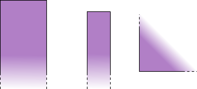
Two rectangles and are of the same type if and are bounded for every . For , we have four types of rectangles:
- •
intervals of finite length
- •
intervals of the form or
- •
intervals of the form or
- •
,
for some . We see that for , rectangles and are of the same type if and are of the same type for all . Examples of -dimensional rectangles are given in Figure 3.
In [13], decorated numbers were introduced. These are endpoints of intervals ‘decorated’ with a plus or minus sign depending on whether the endpoints are included in the interval or not. Let . A decorated number is of the form or , where .33 3 The decorated numbers and are never used, as no interval contains points at infinity, but it does not matter whether we include these two points in the definition. The notation is as follows for :
- •
if
- •
if
- •
if
- •
if .
We define decorated points in dimensions for as tuples , where all the ’s are decorated numbers. For an -dimensional rectangle and decorated points and , we write if for all . We define and as the decorated points for which . We write for decorated numbers with unknown ‘decoration’, so is either or .
There is a total order on the decorated numbers given by for , and for all . This induces a poset structure on decorated -dimensional points given by if for all . We can also add decorated numbers and real numbers by letting and for , . We add -dimensional decorated points and -tuples of real numbers coordinatewise.
If is an interval decomposable -module and all are rectangles, is rectangle decomposable.
Our goal is to prove the following theorem:
Theorem 4.2.
Let and be rectangle decomposable -modules. If and are -interleaved, there exists a -matching between and .
The inequality for rectangle decomposable modules and immediately follows.
Fix . Assume that and are -interleaved, with interleaving morphisms and . Recall that this means that and . For any , we have a canonical injection and projection , and likewise, we have canonical morphisms and for . We define
| (4) | ||||
We prove the theorem by a mix of combinatorial and geometric arguments. First we show that it is enough to prove the theorem under the assumption that all the rectangles in and are of the same type. Then we define a real-valued function on the set of rectangles which in a sense measures, in the case , how far ‘up and to the right’ a rectangle is. There is a preorder associated to . The idea behind is that if there is a nonzero morphism and , then and have to be close to each other. Finding pairs of intervals in and that are close is exactly what we need to construct a -matching. Lemmas 4.6 and 4.7 say that such morphisms behave nicely in a precise sense that we will exploit when we prove Lemma 4.8. If we remove the conditions mentioning , Lemmas 4.6 and 4.7 are not even close to being true, so one of the main points in the proof of Lemma 4.8 is that we must exclude the cases that are not covered by Lemmas 4.6 and 4.7. We do this by proving that a certain matrix is upper triangular, where the ‘bad cases’ correspond to the elements above the diagonal and the ‘good cases’ correspond to elements on and below the diagonal.
Lemma 4.8 is what ties together the geometric and combinatorial parts of the proof of Theorem 4.2. While we prove Lemma 4.8 by geometric arguments, by Hall’s marriage theorem the lemma is equivalent to a statement about matchings between and . We have to do some combinatorics to get exactly the statement we need, namely that there is a -matching between and , and we do this after stating Lemma 4.8.
We begin by describing morphisms between rectangle modules.
Lemma 4.3.
Let be a morphism between interval modules. Suppose is an interval. Then, for all , as -endomorphisms.
Proof.
Suppose and . Then . Since the -morphisms are identities, we get as -endomorphisms. By the connectivity axiom for intervals, the equality extends to all elements in . ∎
Since the intersection of two rectangles is either empty or a rectangle, we can describe a morphism between two rectangle modules uniquely as a -endomorphism if their underlying rectangles intersect. A -endomorphism, in turn, is simply multiplication by a constant. Note that we could have relaxed the assumptions in the proof above and assumed that is in instead of in , and still have gotten . In particular, this means that if , and and are rectangles, then for all , which gives . Similarly, , and one can also see that must hold, or else . We summarize these observations as a corollary of Lemma 4.3:
Corollary 4.4.
Let and be rectangles, and let be a nonzero morphism. Then and .
We define a function by letting if is given by multiplication by , and if is the zero morphism. is given by in the same way.
With the definition of , it is starting to become clear how combinatorics comes into the picture. We can now construct a bipartite weighted directed graph on by letting be the weight of the edge from to . The reader is invited to keep this picture in mind, as a lot of what we do in the rest of the proof can be interpreted as statements about the structure of this graph.
The following lemma allows us to break up the problem and focus on the components of and with the same types separately.
Lemma 4.5.
Let and be rectangles of the same type, and be a rectangle of a different type. Then for any pair , of morphisms.
Proof.
Suppose . By Corollary 4.4, and . We get and for all , and it follows that if and are of the same type, then is of the same type as and . ∎
Let be defined by for and if and are of the same type, and if they are not, and let be defined analogously. Here and are assembled from and the same way and are from and . Suppose . Then we have
| (5) | ||||
When and are of different types, the left side is zero because and are -interleaving morphisms, and all the summands on the right side are zero by definition of and . When and are of the same type, the equality follows from Lemma 4.5. This means that . We also have , so and are -interleaving morphisms. In particular, and are -interleaving morphisms when restricted to the components of and of a fixed type. If we can show that and induce a -matching on each of the mentioned components, we will have proved Theorem 4.2. In other words, we have reduced the problem to the case where all the intervals in and are of the same type.
For a decorated number , let if and otherwise. Let be a decorated point. We define to be the number of the decorated numbers decorated with , and we also define . What we really want to look at are rectangles and not decorated points by themselves, so we define and for any rectangle . Define an order on decorated points given by if either
- •
, or
- •
and
This defines a preorder. In other words, it is transitive ( implies ) and reflexive ( for all ). We write if and not .
The order is one of the most important ingredients in the proof. The point is that if there is a nonzero morphism from to and , then and have to be close to each other. If , and actually have to be equal. This ‘closeness property’ is expressed in Lemma 4.6, and is also exploited in Lemma 4.7. Finally, in the proof of Lemma 4.8, we make sure that we only have to deal with morphisms for and not , so that our lemmas can be applied.
In Figure 4 we see two rectangles and . There is no nonzero morphism from to or , because for all . This is connected to the fact that , which can be interpreted to mean that is ‘further down and to the left’ than . The point of including in the definition of is that e.g. is a tiny bit ‘further to the right’ than , and this is a subtlety that recognizes, and that matters in the proofs of Lemmas 4.6 and 4.7.

Lemma 4.6.
Let , , and be rectangles of the same type with . Suppose there are nonzero morphisms and . Then is -interleaved with either or .
Proof.
Suppose and are not -interleaved. Then either or ; let us assume the latter. (The former is similar.) In this case, there is an such that . For , we have by the second bullet point. We get
| (6) | ||||
The first bullet point gives us
| (7) |
so we get . If the inequality is strict, we have . If not, we have
- •
for all
- •
for
- •
.
Because of the inequalities and (recall that these are inequalities of decorated points with the poset structure we defined earlier), we have for all and for . But since , we have , so . Similarly, we can prove if and are not -interleaved, so we have , which is a contradiction. ∎
Lemma 4.7.
Let , , and be rectangles of the same type with and -significant and . Suppose there are nonzero morphisms and . Then .
The constant can be improved on for , but since the constant in Lemma 4.6 is optimal, strengthening Lemma 4.7 will not help us get a better constant in Theorem 4.2.
Proof.
Suppose that and are nonzero, but . We have
- •
- •
for some
- •
- •
.
The first and third statements hold because . (See Corollary 4.4.) The second is equivalent to . If this did not hold, and would intersect, and would be nonzero in this intersection, which is a contradiction. The fourth statement follows from the second and the fact that is -significant.
Since is -significant, . Thus the second bullet point implies that . The first point gives for . In a similar fashion, we get from the last two points that and for . From all this, we get
| (8) | ||||
Equality only holds if , , and . This means that . As we see, , so . ∎
We define a function by
| (9) |
for in . In other words, contains all the intervals that can be matched with in a -matching. Let be -significant, and pick such that . Then, for every . Since and are p.f.d., this means that is a finite set. For , we write .
Lemma 4.8.
Let be a finite subset of containing no -trivial elements. Then .
Before we prove Lemma 4.8, we show that it implies that there is a -matching between and and thus completes the proof of Theorem 4.2.
Let be the undirected bipartite graph on with an edge between and if . Observe that is the same as the graph we defined when we gave the graph theoretical definition of an -matching (in this case, -matching) in section 2. Following that definition, a -matching is a matching in that covers the set of all -significant elements in and .
For a subset of a graph , let be the neighbourhood of in , that is, the set of vertices in that are adjacent to at least one vertex in . We now apply Hall’s marriage theorem [18] to bridge the gap between Lemma 4.8 and the statement we want to prove about matchings.
Theorem 4.9 (Hall’s theorem).
Let be a bipartite graph on bipartite sets and such that is finite for all . Then the following are equivalent:
- •
for all ,
- •
there exists a matching in covering .
One of the two implications is easy, since if for some , then there is no matching in covering . It is the other implication we will use, namely that the first statement is sufficient for a matching in covering to exist.
Letting be the set of -significant intervals in and be , Hall’s theorem and Lemma 4.8 give us a matching in the graph covering all the -significant elements in .44 4 Strictly speaking, Lemma 4.8 says nothing about infinite , but the case with countably infinite follows from the finite cases. Each interval in contains a rational point, so since is p.f.d., the cardinality of is at most finite times countably infinite, which is countable. Thus we have covered all the possible cases. By symmetry, we also have a matching in covering all the -significant elements in . Neither of these is necessarily a -matching, however, as each of them only guarantees that all the -significant intervals in one of the barcodes are matched. We will use and to construct a -matching. This construction is similar to one used to prove the Cantor-Bernstein theorem [1, pp. 110-111].
Let be the undirected bipartite graph on for which the set of edges is the union of the edges in the matchings and . Let be a connected component of . Suppose the submatching of in does not cover all the -significant elements of . Then there is a -significant that is not matched by . If we view and as partial bijections and , we can write the connected component of , which is , as . Either this sequence is infinite, or it is finite, in which case the last element is -trivial. In either case, we get that the submatching of in covers all -significant elements in .
By this argument, there is a -matching in each connected component of . We can piece these together to get a -matching in , so Lemma 4.8 completes the proof of Theorem 4.2.
Proof of Lemma 4.8.
Because is a preorder, we can order so that for all . Write . For , we have
| (10) | ||||
Also, for , since is zero between different components of . Lemma 4.6 says that if and , then is -interleaved with either or . This means that if , then
| (11) | ||||
as for all that are not -interleaved with either or . Similarly,
| (12) | ||||
Writing this in matrix form, we get
That is, on the right-hand side we have the internal morphisms of the on the diagonal, and below the diagonal.
Recall that a morphism between rectangle modules can be identified with a -endomorphism, and that in our notation, and are given by multiplication by and , respectively. For an arbitrary morphism between rectangle modules, we introduce the notation if is given by multiplication by , and otherwise. A consequence of Lemma 4.7 is that whenever , in particular if . We get
| (13) | ||||
and similarly for . Again we can interpret this as a matrix equation:
That is, the right-hand side is an upper triangular matrix with ’s on the diagonal. The right-hand side has rank and the left-hand side has rank at most , so the lemma follows immediately from this equation. ∎
4.2 Block decomposable modules
Next, we prove stability for block decomposable modules, which, as explained in Section 3, implies stability for zigzag modules and Reeb graphs. Let .
Definition 4.10.
A triangle is a nonempty set of the form for some with .
It follows that triangles are intervals. For a triangle , we write . If is bounded, is the maximal element in the closure of , as illustrated in Figure 5. A triangle decomposable module is an interval decomposable -module whose barcode only contains triangles. Observe that triangles correspond exactly to blocks of the form under the poset isomorphism between and flipping the -axis.

Theorem 4.11.
Let and be -interleaved triangle decomposable modules. Then there is a -matching between and .
To prove this, we can split the triangles into sets of different ‘types’, as we did with the rectangles. We get four different types of triangles , depending on whether is of the form , , , or for . Now a result analogous to Lemma 4.5 holds, implying that it is enough to show Theorem 4.11 under the assumption that the barcodes only contain intervals of a single type. The case in which the triangles are bounded is the hardest one, and the only one we will prove. So from now on, we assume all triangles to be bounded.
Again, we reuse parts of the proof of Theorem 4.2. For , we define . The discussion about Hall’s theorem is still valid, so we only need to prove the analogue of Lemma 4.8 for . Define , where . The only things we need to complete the proof of the analogue of Lemma 4.8 for triangle decomposable modules are the following analogues of Lemmas 4.6 and 4.7:
Lemma 4.12.
Let , , and be triangles with . Suppose there are morphisms and such that . Then is -interleaved with either or .
Lemma 4.13.
Let , , and be triangles with -significant and . Suppose there are nonzero morphisms and . Then .
Proof of Lemma 4.12.
Suppose and are not -interleaved. Then . But at the same time, , which gives . Assuming that and are not -interleaved, either, we also get . Thus , a contradiction. ∎
Proof of Lemma 4.13.
For all triangles , we treat and as undecorated points. We have and , so . Because is -significant, for some . Combining these facts, we get , so . ∎
Theorem 4.11 implies for block decomposable and such that and only have blocks of the form (so no closed or half-closed blocks). Our proof technique extends easily to prove the same equality for all block decomposable and . In fact, in the case where all the intervals in the barcodes are of the form follows from Theorem 4.16 below with by the correspondence , while the two cases with half-open blocks are both essentially the algebraic stability theorem. In the end we could stitch the cases together by something similar to Lemma 4.5 and the discussion following it. We omit the details, and anyway the closed and half-open cases are taken care of in [3]. Thus, either by appealing to previous work for the other cases or using our own methods, we get
Theorem 4.14.
Let and be block decomposable modules. If and are -interleaved, there exists a -matching between and .
4.3 Free modules
Definition 4.15.
We define a free interval as an interval of the form .
For a free interval , we define by .55 5 This makes an undecorated point, while we have previously defined as decorated points, but this does not matter, as we will not need decorated points in this subsection. We define a free -module as an interval decomposable module whose barcode only contains free intervals. It is easy to see that free intervals are rectangles, so it follows from Theorem 4.2 that for free modules , . But because of the geometry of free modules, this result can be strengthened.
Theorem 4.16.
Let and be free -interleaved -modules with . Then there is a -matching between and .
We already did most of the work while proving Theorem 4.2, and there are some obvious simplifications. Firstly, free intervals are -significant for all . Secondly, for all nonzero and with , , free, is nonzero. For , define . By the arguments in the proof of Theorem 4.2, we only need to prove Lemma 4.8 with replaced by . Lemmas 4.6 and 4.7 still hold for free modules, but we need to sharpen Lemma 4.6.
Lemma 4.17.
Let , , and be free intervals with . Suppose there are morphisms and . Then is -interleaved with either or .
Proof.
In this proof, we treat and as undecorated points for all free intervals , so that we can add them. We have . Suppose and are not -interleaved. Then , so for some , we must have . We get
| (14) | ||||
We can also prove that if and are not -interleaved, so we have , a contradiction. ∎
5 Counterexamples to a general algebraic stability theorem
Theorem 4.2 gives an upper bound of on for rectangle decomposable modules that increases with the dimension. An obvious question is whether it is possible to improve this constant, or if for each there exist pairs of modules for which , in which case the bound is optimal. We know that for any and whenever the bottleneck distance is defined, so for , the constant is optimal. For , however, it turns out that the equality does not always hold, and the geometry becomes more confusing when increases. In dimension , we give an example of rectangle decomposable modules and with in Example 5.2, which means that the bound is optimal for , as well. This is a counterexample to a conjecture made in a previous version of [3] which claims that interval decomposable -modules and such that and only contain convex intervals are -matched if they are -interleaved.
Example 5.1.
Let 66 6 Here we use subscripts to index different intervals, not to indicate projections, as we did earlier. and , where
- •
- •
- •
- •
.

See Figure 6. We can define -interleaving morphisms and by letting and , where is defined as in the proof of Theorem 4.2. On the other hand, in any matching between and we have to leave either or unmatched, and they are -significant for all . In fact, any possible matching between and is a -matching. Thus and .
A crucial point is that even though , , , and are all nonzero, both and are zero. To do the same with one-dimensional intervals, we would have to shrink and so much that they no longer would be -significant (see Lemma 4.7), and then they would not need to be matched in a -matching. This shows how the geometry of higher dimensions can allow us to construct examples that would not work in lower dimensions.
Next, we give an example of rectangle decomposable -modules and such that , proving that our upper bound of is the best possible for .
Example 5.2.

We give an example of -interleaving morphisms and that we write on matrix form. In the first matrix, is in row , column . In the second, is in row , column .
| (15) |
This means that and are -interleaved, but they are not -interleaved for any , so .
Let . We see that the difference between and is in the first coordinate, so and are not -interleaved, and thus they cannot be matched in an -matching. In fact, and cannot be matched in an -matching for any by similar arguments. Since and cannot both be matched with , one of them has to be left unmatched, but since both and are -significant, this means that there is no -matching between and . On the other hand, any bijection between and is a -matching, so .
There is a strong connection between -dimensional rectangle decomposable modules and -dimensional free modules. This is related to the fact that we need coordinates to determine an -dimensional rectangle, and also coordinates to determine a -dimensional free interval. The following example illustrates this connection, as we simply rearrange the coordinates of , for all rectangles involved in Example 5.2 to get -dimensional free modules with similar properties as in Example 5.2.
Example 5.3.
As a consequence of this example, we get that our upper bound of for free -dimensional modules cannot be improved on for .
6 Relation to the complexity of calculating interleaving distance
The interleaving distance between arbitrary persistence modules is on the surface not easy to find, as naively trying to construct interleaving morphisms can quickly lead you to consider a complicated set of equations for which it is not clear that one can decide if there is a solution in polynomial time. For -modules, however, the interval decomposition theorem plus the algebraic stability theorem gives us a polynomial time algorithm to compute : decompose the modules into intervals and find the bottleneck distance. Since , this gives us the interleaving distance. When it exists, one can compute the bottleneck distance in polynomial time also in two dimensions [17], but the approach fails for general -modules already at the first step, as we do not have a nice decomposition theorem. But in the recent proof that calculating interleaving distance is NP-hard [9], it is the failure of the second step that is exploited. Specifically, a set of modules that decompose nicely into interval modules (staircase modules, to be precise) is constructed, but for these, and are different. It turns out that calculating for these corresponds to deciding whether CI problems are solvable, which is shown to be NP-hard.
Though rectangle modules are not considered in the NP-hardness proof, they have similar properties to staircase modules,77 7 The only significant difference in this setting is that in a fixed dimension, rectangle modules are defined by a limited number of coordinates, or “degrees of freedom”, while there is no such restriction on staircase modules even in dimension . and Example 5.2 is essentially a CI problem with a corresponding pair of modules. Importantly, it shows that does not hold in general for modules corresponding to CI problems. This crucial observation, which appeared first in a preprint of this paper [8], opened the door to proving NP-hardness of calculating by the approach used in [9].
In [9], it is also shown that -approximating is NP-hard for , where an algorithm is said to -approximate if it returns a number in the interval for any input pair , of modules. Whether the approach by CI problems can be used to prove hardness of -approximation for is closely related to Theorem 4.2. It can be shown that if for any pair , of rectangle decomposable modules, the same holds for staircase modules, and therefore there is a polynomial time algorithm -approximating for these, meaning that the strategy of going through CI problems will not give a proof that -approximation of is NP-hard. On the other hand, if one can find an example of rectangle decomposable modules and such that for , one might be able to use that to increase the constant in the approximation hardness result. Thus there is a strong link between stability of rectangle decomposable modules and the only successful method so far known to the author of determining the complexity of computing or approximating multiparameter interleaving distance.
7 Acknowledgements
I would like to thank my supervisors Gereon Quick and Nils Baas for invaluable support and help. I would also like to thank Peter Landweber for detailed comments on several drafts of this text, Steve Oudot for feedback on the first arXiv version and Magnus Bakke Botnan for interesting discussions.
References
- [1] Martin Aigner and Günter M. Ziegler. Proofs from THE BOOK. Springer, Berlin, 4th edition, 2010.
- [2] Gorô Azumaya. Corrections and supplementaries to my paper concerning Krull-Remak-Schmidt’s theorem. Nagoya Mathematical Journal, 1:117–124, 1950.
- [3] Magnus Bakke Botnan and Michael Lesnick. Algebraic stability of zigzag persistence modules. Algebraic & Geometric Topology, 18, 04 2016.
- [4] Ulrich Bauer, Xiaoyin Ge, and Yusu Wang. Measuring distance between reeb graphs. In Proceedings of the thirtieth annual symposium on Computational geometry, page 464. ACM, 2014.
- [5] Ulrich Bauer and Michael Lesnick. Induced matchings and the algebraic stability of persistence barcodes. Journal of Computational Geometry, 6(2):162–191, 2015.
- [6] Ulrich Bauer, Elizabeth Munch, and Yusu Wang. Strong Equivalence of the Interleaving and Functional Distortion Metrics for Reeb Graphs. In 31st International Symposium on Computational Geometry (SoCG 2015), volume 34 of Leibniz International Proceedings in Informatics (LIPIcs), pages 461–475. Schloss Dagstuhl–Leibniz-Zentrum fuer Informatik, 2015.
- [7] Paul Bendich, Herbert Edelsbrunner, Dmitriy Morozov, Amit Patel, et al. Homology and robustness of level and interlevel sets. Homology, Homotopy and Applications, 15(1):51–72, 2013.
- [8] Håvard Bakke Bjerkevik. Stability of higher-dimensional interval decomposable persistence modules. arXiv preprint arXiv:1609.02086v2, 2016.
- [9] Håvard Bakke Bjerkevik, Magnus Bakke Botnan, and Michael Kerber. Computing the interleaving distance is np-hard. arXiv preprint arXiv:1811.09165, 2018.
- [10] Gunnar Carlsson and Vin De Silva. Zigzag persistence. Foundations of computational mathematics, 10(4):367–405, 2010.
- [11] Gunnar Carlsson, Vin De Silva, and Dmitriy Morozov. Zigzag persistent homology and real-valued functions. In Proceedings of the twenty-fifth annual symposium on Computational geometry, pages 247–256. ACM, 2009.
- [12] Frédéric Chazal, David Cohen-Steiner, Marc Glisse, Leonidas J Guibas, and Steve Y Oudot. Proximity of persistence modules and their diagrams. In Proceedings of the twenty-fifth annual symposium on Computational geometry, pages 237–246. ACM, 2009.
- [13] Frédéric Chazal, Vin De Silva, Marc Glisse, and Steve Oudot. The structure and stability of persistence modules. Springer, 2016.
- [14] David Cohen-Steiner, Herbert Edelsbrunner, and John Harer. Stability of persistence diagrams. Discrete & Computational Geometry, 37(1):103–120, 2007.
- [15] William Crawley-Boevey. Decomposition of pointwise finite-dimensional persistence modules. Journal of Algebra and Its Applications, 14(05):1550066, 2015.
- [16] Vin De Silva, Elizabeth Munch, and Amit Patel. Categorified reeb graphs. Discrete & Computational Geometry, 55(4):854–906, 2016.
- [17] Tamal K. Dey and Cheng Xin. Computing Bottleneck Distance for 2-D Interval Decomposable Modules. In 34th International Symposium on Computational Geometry (SoCG 2018), volume 99 of Leibniz International Proceedings in Informatics (LIPIcs), pages 32:1–32:15. Schloss Dagstuhl–Leibniz-Zentrum fuer Informatik, 2018.
- [18] Philip Hall. On representatives of subsets. J. London Math. Soc, 10(1):26–30, 1935.
- [19] Woojin Kim and Facundo Memoli. Stable signatures for dynamic metric spaces via zigzag persistent homology. arXiv preprint arXiv:1712.04064, 2017.
- [20] Steve Y Oudot and Donald R Sheehy. Zigzag zoology: Rips zigzags for homology inference. Foundations of Computational Mathematics, 15(5):1151–1186, 2015.
- [21] Cary Webb. Decomposition of graded modules. Proceedings of the American Mathematical Society, 94(4):565–571, 1985.