Brane Brick Models in the Mirror
Abstract
Brane brick models are Type IIA brane configurations that encode the gauge theories on the worldvolume of D1-branes probing toric Calabi-Yau 4-folds. We use mirror symmetry to improve our understanding of this correspondence and to provide a systematic approach for constructing brane brick models starting from geometry. The mirror configuration consists of D5-branes wrapping 4-spheres and the gauge theory is determined by how they intersect. We also explain how triality is realized in terms of geometric transitions in the mirror geometry. Mirror symmetry leads to a geometric unification of dualities in different dimensions, where the order of duality is for a Calabi-Yau -fold. This makes us conjecture the existence of a quadrality symmetry in . Finally, we comment on how the M-theory lift of brane brick models connects to the classification of theories in terms of 4-manifolds.
1 Introduction
The interplay between Calabi-Yau (CY) geometry and branes probing it has played a key role in understanding duality symmetries of field theories that emerge in string theory. More specifically D-branes probing CY singularities have given rise to an interesting class of SCFT’s. In particular, D3-branes probing CY 3-folds lead to theories (see e.g. [1, 2, 3, 4, 5, 6, 7] and references therein). It was shown in [8] that one can use the mirror symmetry of CY 3-folds to not only understand what the corresponding quiver theory is, but also to understand Seiberg dualities between them as a continuous change of parameters in the mirror geometry.
More recently, D1-branes probing CY 4-fold singularities were considered in [9, 10, 11], where the corresponding gauge theories they give rise to were proposed. These theories lead to SCFT’s. Moreover, in this context it was proposed in [12] that these theories enjoy triality symmetries, which is rather novel. The main goal of this paper is to extend the observation about applying mirror symmetry in the context of D3-branes probing CY 3-folds to demystify those theories: we use mirror symmetry to not only explain what the prescription of the resulting quiver is, but also explain triality using the mirror geometry. In a subsequent paper we show that this extends to the case of D(-1) instantons probing CY 5-folds, but now mirror symmetry leads to a quadrality symmetry [13].
Let us sketch the basic idea for a Calabi-Yau -fold. Consider a D-brane probing the CY singularity. Let us first move the brane away from the singular locus. Note that the position of the D-brane in the transverse space is a point in the CY. Now we apply mirror symmetry, which converts the D-brane to wrap in addition an -dimensional torus , as in the SYZ picture of mirror symmetry [14]. Now we move the position of the brane to the singular point. At the singular point, the breaks up to subspaces. From the geometry of the subspaces we can infer the resulting quiver gauge theory.
The simplest example is when , and we are probing an singularity with D5-branes. In this case, as the D5-brane approaches the singular locus, the mirror breaks up to a necklace of spheres touching one another at a point. This gives rise the usual quiver description. Namely, for D5-branes probing it, we get each sphere being wrapped by D-branes giving the gauge group with bifundamental matter from their neighboring intersections, leading to an affine quiver theory. We view this geometry as an fibration over a base . The base will be depicted by a circle, broken by points which denotes the loci where the fiber shrinks. So each of the intervals on corresponds to a sphere and the neighboring intervals will have a bifundamental matter field in common.
The same story repeats for any -fold. In the general case, the mirror fiber will be viewed as an fibration over a geometry. Loci where shrinks break up the into regions, each of which will correspond to a gauge factor. The neighboring regions will lead to matter bifundamentals. The codimension-2 interfaces where the codimension-1 faces meet lead to loci where interactions take place between matter multiplets. From this structure we can read off the quiver theory, its matter content and its interactions.
To read off dualities, we use the complex mirror geometry and consider changing the complex structure. The inequivalent geometries we obtain correspond to complex deformations and passing through vanishing cycles. However the mirror geometry unifies the inequivalent geometries of the Calabi-Yau into a single Calabi-Yau manifold as is familiar from various examples of mirror symmetry. In this way we can read off dualities by the uniqueness of the Calabi-Yau mirror. We find that for the -fold case we get generalized duality symmetries which return to the original theory after steps. So for 2-fold case, we get the usual Weyl reflection which is the self-duality of with flavors [15], for the 3-fold case we get Seiberg duality [16], for the 4-fold case we get the triality of Gadde, Gukov and Putrov [12], and for the 5-fold case we get a quadrality [13]. The order of the symmetry is easiest to see in the context of the local Calabi-Yau given by bundle over .
The organization of this paper is as follows. Section §2 reviews theories, D1-branes over toric CY 4-folds and brane brick models. Section §3 presents a general discussion of the mirror of D-branes probing CY -folds. Section §4 specializes on D3-branes probing toric CY 3-folds. Section §5 discusses the application of mirror symmetry to D1-branes probing toric CY 4-folds in detail and explains how to use it for constructing the corresponding brane brick models. Additional examples are presented in section §6. Section §7 explains how triality arises from geometric transitions in the mirror. Section §8 connects to the classification of theories in terms of 4-manifolds in the M-theory lift of brane brick models. We present our conclusions in section §9. In two appendices we present additional examples and details about the open string spectrum at D-brane intersections.
2 Brane Brick Models and Theories
This paper is mainly devoted to the gauge theories that arise on the worldvolume of D1-branes probing singular toric CY 4-folds. This section contains a brief review of general theories, the special structure of the theories on D1-branes on toric CY 4-folds and brane brick models. We refer the reader to [9, 10, 11], where the ideas presented below were originally introduced.
2.1 Gauge Theories
In order to set up the language, let us quickly review some basic aspects of gauge theories. Thorough introductions to the subject can be found in [17, 18, 12, 19]. These theories can be efficiently formulated in terms of superspace , . Their elementary building blocks are three types of superfields:
- •
Vector: it contains a gauge boson , adjoint chiral fermions , and an auxiliary field . Here and in what follows, subindices indicate the chirality of the corresponding fermions.
- •
Chiral: the component expansion and chirality condition of a chiral field take the form
(2.1) The on-shell degrees of freedom are a complex scalar and a chiral fermion , and is a supercovariant derivative.
- •
Fermi: the chirality condition of a Fermi field may be deformed by a holomorphic function of chiral fields , which gives rise to interactions among matter fields. Fermi fields have the following component expansion
(2.2) is an auxiliary field and the chiral fermion is the only on-shell degree of freedom.
Let us now discuss some important building blocks of the Lagrangian. The kinetic terms for the Fermi multiplets plus some interactions of matter fields arise from
| (2.3) |
where runs over the Fermi fields of the theory.
Interactions among matter fields can also be incorporated via the couplings
| (2.4) |
where the are holomorphic functions of chiral fields. In summary, every Fermi field is associated to a pair of holomorphic functions of chiral fields and . Consistency of the theory requires - and -terms satisfy the following constraint
| (2.5) |
Integrating out the auxiliary components in the Fermi fields, and give rise to the following contributions to the scalar potential11 1 The scalar potential contains additional positive definite contributions from the D-terms in vector multiplets.
| (2.6) |
and to interactions between scalars and pairs of fermions
| (2.7) |
theories are invariant under the swap for any , accompanied with the exchange .
In this paper, we focus on theories in which all fields transform in either bifundamental or adjoint representations of a gauge group and can hence be represented by quiver diagrams as shown in Figure 1.
2.2 D1-Branes over Toric Calabi-Yau 4-Folds and Brane Brick Models
We will focus on the theories that arise on the worldvolume of Type IIB D1-branes probing toric CY 4-folds. The probed CY4 arises as the classical mesonic moduli space of the gauge theory. More precisely, for D1-branes, this moduli space is the algebraic variety
| (2.8) |
where and run over the chiral and Fermi fields, respectively, and is the number of gauge groups. is equal to the volume of the toric diagram of the CY4, normalized with respect to a minimal tetrahedron. Vanishing of the scalar potential requires the individual vanishing of -, - and -terms. is the symmetric product of the probed CY4, . For gauge groups, the variety in (2.8) becomes exactly the probed CY4.
A new class of Type IIA brane configuration, denoted brane brick models was introduced in [10]. Brane brick models are related to D1-branes over toric CY4 singularities by T-duality along three directions. Brane brick models substantially simplify and offer a new perspective on the connection between the CY4 geometry and the corresponding gauge theories. By doing so, they also provide a powerful tool for studying the dynamics of theories.
A brane brick model consists of D4-branes suspended from an NS5-brane. The NS5-brane extends along the directions and wraps a holomorphic surface embedded into the directions. The directions are periodically identified to form a 3-dimensional torus. The coordinates , and are pairwise combined into three complex variables , and . The corresponds to the arguments of these complex variables, . is defined as the zero locus of the Newton polynomial associated to the toric diagram of the CY4, . Stacks of D4-branes extend along and are suspended inside the holes cut out by on the torus. The R-symmetry of the gauge theories corresponds to rotations on the plane, on which all the branes sit at a point. Table 1 summarizes the structure of a brane brick model.
| 0 | 1 | 2 | 3 | 4 | 5 | 6 | 7 | 8 | 9 | |
|---|---|---|---|---|---|---|---|---|---|---|
| D4 | ||||||||||
| NS5 | ———– ———— | |||||||||
It is convenient to represent a brane brick model by its “skeleton” on . We will often refer to this simplified object also as the brane brick model. Every brane brick model defines a gauge theory according to the rules in Table 2. Bricks correspond to gauge groups.22 2 Having different ranks is possible if fractional D1-branes are introduced in the T-dual configuration of branes at a CY4 singularity. There are two types of faces, representing to the two types of matter superfields present in theories. Every oriented face corresponds to chiral field and every unoriented face represents a Fermi field and its conjugate . Throughout this paper, we will distinguish chiral and Fermi faces by coloring them grey and red, respectively. Fermi faces are 4-sided, this follows from the special structure of - and E-terms in toric theories, as explained below. Figure 2 illustrates the correspondence between brane brick models and gauge theories using the local example.
| Brane Brick Model | Theory |
|---|---|
| Brick | Gauge group |
| Oriented face between bricks | Chiral field in the bifundamental representation |
| and | of nodes and (adjoint for ) |
| Unoriented square face between | Fermi field in the bifundamental representation |
| bricks and | of nodes and (adjoint for ) |
| Edge | Plaquette encoding a monomial in a |
| - or -term |

In the theories dual to toric CY4’s, - and -terms have a special structure, which was dubbed the toric condition in [9]. In these theories, the - and -terms take the form
| (2.9) |
with and holomorphic monomials in chiral fields.33 3 More precisely, the toric condition holds in those phases of the gauge theory that are described by brane brick models, which are often referred to as toric phases. Non-toric phases can be reached by general triality transformations, as explained in section §7. In such phases, the ranks of all gauge nodes are no longer equal and the - and -terms do not necessarily obey the toric condition. The origin of the toric condition can be understood geometrically. Toric CY4’s are defined by monomial relations, and these are precisely the type of relations that arise from vanishing - and -terms when they are of the form (2.9). The toric condition has an alternative, more physical, derivation in terms of classical higgsing [9]. Higgsing corresponds to partial resolution of the probed geometries and can be systematically exploited for obtaining the gauge theory for an arbitrary toric CY4’s starting from the one for an abelian orbifold of . The identification of edges in the brane brick model with monomials in - and -terms, together with the toric condition, imply that the faces associated to Fermi fields are 4-sided, as already anticipated.
Brane brick models are in one-to-one correspondence with periodic quivers on , which automatically incorporate the toric condition. Periodic quivers not only encode the gauge symmetry and matter content of toric theories, but also their - and -terms [9]. The latter are represented by minimal plaquettes. A plaquette is defined as a gauge invariant closed loop in the quiver consisting of an oriented path of chiral fields and a single Fermi field. The toric condition implies that every Fermi is associated to four minimal plaquettes as shown in Figure 3. The full periodic quiver is constructed by assembling together all fields according to their minimal plaquettes. Brane brick models and periodic quivers are simply related by graph dualization, as shown in Figure 2.

3 Mirror Approach to Brane Tilings and Brane Brick Models
A central goal of this paper is to develop the mirror description for configurations of D1-branes probing toric CY 4-folds. The use of mirror symmetry for this purpose was pioneered in [20], in the context of D3-branes over toric CY 3-folds. There results were later generalized to toric CYn singularities with arbitrary in a beautiful paper by Futaki and Ueda [21]. Here we present the basics of this construction. A detailed analysis of the and cases is given in sections §4 and §5.
Every toric CYn is specified by its toric diagram , which is a convex set of points . Its mirror geometry [22, 23] is another -fold given by a double fibration over the complex plane
| (3.10) |
with and , . Here is the Newton polynomial associated to the toric diagram
| (3.11) |
where the are complex coefficients and the sum runs over points in the toric diagram. It is possible to scale of the coefficients to 1.
The critical points of are defined as such that
| (3.12) |
and, on the -plane correspond to the critical values . In [20] it was proved that for arbitrary , when the toric diagram contains at least one internal point, the number of critical points of matches the normalized volume of the toric diagram.44 4 Throughout the paper we will focus on toric diagrams that satisfy this condition. We are confident that our ideas can be extended to toric diagrams without internal points. The number of critical points is precisely the one required for a basis of wrapped D-branes in the mirror that accounts for the gauge nodes in the field theory, for any .
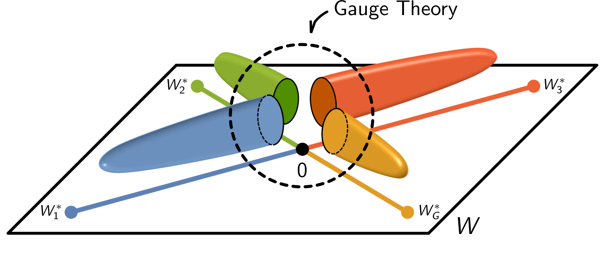
The fiber associated to corresponds to a holomorphic -complex dimensional surface , while the one is a fibration. For generic values of the coefficients, an shrinks to zero size at each critical value . In addition, the from the fibration vanishes at . Considering this fibration over a straight vanishing path connecting and , we obtain an , as illustrated in Figure 4.55 5 In section §7 and appendix §A we will comment on the possibility of non-straight vanishing paths on the -plane.

All the ’s meet at , where the fiber vanishes. The gauge theory is encoded in the way the ’s intersect on the vanishing locus , as illustrated in Figure 5. For this is precisely the holomorphic surface that underlies the brane tiling [24] and the brane brick model, as we explained in section §2.2. This implies that these objects can be reconstructed from the intersections of the ’s. We will refer to each as , , and to the corresponding on as . When studying the intersections of the , it is often useful to consider two standard projections: the amoeba, which projects onto the -plane, and the coamoeba, which projects it on the -torus.
Tomography.
A useful tool for analyzing the mirror, to which we refer as tomography, was introduced in [21]. The -tomography is the projection of the configuration of spheres at on the -plane. The coamoeba projection of the -tomographies provides a powerful systematic algorithm for constructing brane tilings and brane brick models. An appealing feature of tomography is its scalability. Every time the CY dimension is increased by one, we simply need to include an additional complex plane. In sections §4 and §5, we will discuss tomography in detail with various explicit examples.
4 Calabi-Yau 3-Folds and Brane Tilings
D3-branes over toric CY3 singularities map to a collection D6-branes wrapped over 3-spheres in the mirror [20]. Here we revisit the CY3 case in order to set up the stage for CY4’s, to be considered in section 5, and to illustrate the refined analysis of [21].
4.1
Following [21], we first consider the simplest example: local , i.e. the orbifold with action . The toric diagram for this geometry is shown in Figure 6.
The Newton polynomial has in general four terms. Three of the coefficients can be set to 1, leaving a single tunable parameter. Let us analyze the case in which we set , i.e.
| (4.13) |
As expected, there are three critical points:
| (4.14) |
The critical values are , respectively. To each critical point, we can assign a vanishing path. A vanishing path is a curve on the -plane such that
| (4.15) |
We choose , , to be straight lines connecting the origin to , as shown in Figure 7.
As explained in section §3, every is in one-to-one correspondence with an and with an . D6-branes wrapping the ’s give rise to the gauge theory. In [21], tomography was proposed as a convenient tool for studying the embedding of the into the Riemann surface . Let us consider the -tomography, i.e. let us examine the critical points of as a function of at . We get
| (4.16) |
which we call in order to differentiate them from the critical points of , . Near every critical point , we can locally write
| (4.17) |
Hence, if we consider the inverse function, , becomes a branch point. Explicitly, solving for , we find
| (4.18) |
Thus, the branch points on the -plane are the solutions to . To avoid confusion between in (4.14) and in (4.17), from here on we will refer to the former as critical points and the latter as branch points.
The surface is a branched double cover of the -plane. We should also remember that since is a variable, can also be regarded as a branch point. In fact, as we go around , returns to itself after two turns. The three branch points, together with , give rise to a branched double cover description of a torus with three punctures. This fact was indeed expected, since can be regarded as the “dual” of the toric diagram, which for this example is shown in Figure 6.
Figure 8 illustrates a choice of branch cuts and an example of a non-trivial cycle of the torus. In the figure, we marked the point to emphasize that it is a puncture. (Two other punctures are located at infinity and hence do not appear in the figure.)
contains several 1-cycles. How do we identify , i.e. the one pinching off at a given critical point ? Since the ’s are distinguished by their winding numbers around the branch points and the punctures, we can study what happens as we vary the value of along the corresponding vanishing path . For example, let us consider , along which we have
| (4.19) |
The branch points sit at the solutions to . In particular, at we have a double root at and a simple root at . Recall that is the critical value . Figure 9 shows the evolution of the branch points as goes from to .
Two branch points coalescing into a single point indicate that a cycle is collapsing. It follows that the vanishing cycle corresponding to the vanishing path takes the form shown in Figure 10. The same argument can be repeated to determine and .
The next step is to study the intersections between pairs of vanishing cycles, since they give rise to bifundamental chiral fields in the gauge theory. Let us consider and . In Figure 11, we have slightly deformed the two cycles in order to resolve the individual intersections. Solid and dotted segments lie on two different sheets. Only segments on the same sheet can intersect. We see that and intersect at three points: one near the common branch point and two away from the branch points. Without the deformation, the two bulk intersections would coincide in the -tomography. This is a general property in any dimension: intersections at branch points are always single, while bulk intersections might have higher multiplicity [21]. In fact, in order to get a precise understanding of intersections it is necessary to consider both the - and -tomographies (in general CYn’s, we should take into account all the -tomographies). Sometimes, a pair of cycles might seem to intersect when projected onto some of the planes but another tomography might reveal that they actually never meet. We will illustrate this phenomenon in some of the examples of section §6.
The previous counting, one intersection at a branch point and two in the bulk, holds in any branched double cover descriptions of . We should not, however, get the impression that branch point and bulk intersections are intrinsically different. A branch point on the -plane is not a branch point on the -plane. More generally, we can change the nature of the intersection points by switching among several frames.
Having presented a meticulous description of the geometry of vanishing cycles in the mirror, we can now streamline the discussion as follows. As noted in [21], among the various figures we have discussed, the most important one is Figure 9. As we move on the -plane along a vanishing path , a pair of branch points from converges to at . The union of the two trajectories of branch points, let us call it an arc, defines the vanishing cycle . As shown in Figure 10, is topologically an ; two points fibered over the arc meet at the two branch points, closing the circle. The full -tomography is shown in Figure 12. In principle, it is still necessary to construct the -tomography. In this example, however, it is identical to the -tomography due to the symmetry of (4.13).
It is now possible to systematically build the corresponding brane tiling. The of the brane tiling is precisely the coamoeba torus spanned by . The coamoeba projection maps every fixed value of the argument in a given tomography to a planar slice of . Every vanishing cycle at is mapped to a topologically trivial circle (i.e to the boundary of a disc) on the coameoba . Its “center” is located at the critical point . The intersections between neighboring cycles give rise to chiral fields. The coamoeba diagram [20] is the complement of the union of all discs , whose boundaries are the vanishing cycles . We can immediately construct the brane tiling from the coamoeba, which has a segment for every intersection of ’s, as shown in Figure 13.

4.2
Let us now consider the complex cone over , which is a chiral orbifold of the conifold. For brevity, we will refer to it simply as . This is an interesting example, since it is one of the simplest geometries that admit more than one toric Seiberg dual phases [25, 26]. In , we define a toric phase as one that can be encoded in terms of a brane tiling. Following the detailed presentation in the previous section, the discussion of this example will be more succinct.
The toric diagram for is shown in Figure 14. Let us first consider the following choice of coefficients in the Newton polynomial
| (4.20) |
The four critical points and the corresponding critical values are
| (4.21) |
Figure 15 shows the vanishing paths on the -plane and the - and -tomographies. From them, we can construct the coamoeba diagram and brane tiling, which are shown in Figure 16. They correspond to one of the two toric phases of [25, 26], which we call phase 1.
Interestingly, the second toric phase of can be generated by varying the coefficients in the Newton polynomial. Consider, for example,
| (4.22) |
Comparing (4.20) and (4.22), we note that the coefficient multiplying in the second phase is real. If we set it to 1, two of the critical points would coincide. As long as it is not 1, its absolute value is not important. Another novelty of (4.22) is that it contains a constant term. It prevents the vanishing paths from overlapping. The four critical points and their critical values are now
| (4.23) |
The resulting vanishing paths and - and -tomographies are shown in Figure 17. The corresponding coamoeba and brane tiling are shown in Figure 18. They represent phase 2 of .

A crucial distinction between the mirror configurations describing both phases is the different cyclic orderings of the vanishing paths on the -plane, as shown in Figures 16 and 18. When going from phase 1 to phase 2, , which corresponds to the dualized gauge group, moves over , associated to the node in the quiver from which the flavors going into node emanate. This geometric realization of Seiberg duality was introduced in [8] and will be revisited in section §7, where we generalize it to triality.
5 Calabi-Yau 4-Folds and Brane Brick Models
Having extensively reviewed the application of mirror symmetry to brane tilings, we are ready to explain how a similar approach can be developed for brane brick models. The construction of brane brick model consists of three steps.
First, we identify some compact 2-cycles on the surface as the gauge nodes in complete parallel with brane tilings. Upon double fibration over vanishing paths, they form the compact 4-cycles of the mirror CY4. D5-branes wrapping these 4-cycles give rise to the gauge nodes.
Second, we identify the intersections among the cycles as bifundamental fields of the gauge theory. The fields originate from string segments connecting two different gauge nodes. A main novelty here is that, unlike in brane tilings, there are two distinct types of supermultiplets: chiral and Fermi. We will show that they are distinguished by the orientation of the intersections. A closer look at the oriented intersections can also determine the orientation of the chirals.
Third, we construct the - and -terms that form plaquettes in the brane brick model. Given the coordinates of the gauge nodes and the intersection points in the coamoeba , we will show how to graphically construct all the plaquettes.
In this section, following [21], we will illustrate the ideas with the simplest example: the local (namely the orbifold with action ). We will present additional examples in the next section.
Figure 19 summarizes the basic ingredients in the correspondence between the mirror and brane brick models. We focus on the fibration, leaving the fibration implicit. In red we indicate the brane brick model objects associated with different parts of the mirror. Of course, an analogous picture applies to the connection between D6-branes in the mirror of toric CY 3-folds and brane tilings.

5.1 Cycles as Gauge Nodes
Most of the discussion from the previous section generalizes straightforwardly to CY4. We begin by noting that now defines a four real dimensional hypersurface. As we will see shortly, the vanishing cycles are ’s intersecting with each other transversely.
The main tool for studying and its vanishing cycles is the same as before; we take the tomography of the surface by expressing one of the variables, say , as a function of the other two. Locally, we regard as a fibration over the -plane. At every fixed value of , the fiber , defined by the equation , is a Riemann surface. For a generic value of , is nothing but the Newton polynomial of the projection of the CY4 toric diagram onto the -plane. Hence, we can study the vanishing 2-cycles of the four-dimensional and their intersections by first learning about the fibration structure and then examining how the 1-cycles of the Riemann surface fiber intersect.
Let us consider local , whose toric diagram is shown in Figure 20. The Newton polynomial has in general five terms. Four of the coefficients can be scaled to 1. Setting , we obtain
| (5.24) |
It has four critical points at66 6 In this expression we momentarily use to index cycles in order to avoid confusion with . We will soon return to the notation for cycles in terms of and indices.
| (5.25) |
The vanishing paths, defined in the usual way, are shown in Figure 21.
To construct the -tomography, we study the critical points of as a function of and
| (5.26) |
Although cannot be inverted as (4.17), in order to keep consistency in nomenclature and avoid confusion with in (5.25), we will call branch points. We find four branch points located at
| (5.27) |
As before, we study how these points move as we vary the value of along a vanishing path. We obtain four arcs, each of which is a union of two images of the corresponding vanishing path. The result is shown in Figure 22.
For every value along an arc, we have the Riemann surface fiber , which contains several 1-cycles. One of them pinches off as we approach the two endpoints of the arc. The fibration of the vanishing 1-cycle over the arc defines an . We conclude that each arc in Figure 22 represents an .
How do we determine the intersection number between two of these ’s? We will first focus on the absolute values of the intersection numbers and consider their signs in the coming section. If the ’s meet at a branch point, since both of them shrink to a point there, the local intersection number must be one. If instead the corresponding arcs intersect in the bulk, i.e. away from the branch points, their local intersection number is inherited from that of the 1-cycle on the Riemann surface fiber.
For local , the Riemann surface fiber away from the branch points is always the one of local . Hence, modulo signs, all the bulk intersection numbers are equal to 3. Adding up all contributions, we can summarize the (absolute value of) the intersection numbers as
| (5.28) |
The same analysis applies to the - and -tomographies. In this case, due to the symmetry among , and of the Newton polynomial (5.24), the - and tomographies are identical to Figure 22. The identity of the fields associated to each intersection might differ between tomographies, as we will show in Figure 28.
5.2 Chiral vs Fermi Fields from Oriented Intersections
Intersections between two vanishing cycles give rise to bifundamental fields between two gauge nodes. We will now explain how to distinguish between chiral and Fermi multiplets. In string theory, these fields arise from massless open string modes localized at the intersection. In the current context, a short answer to the field type question is that the signs of oriented intersections determine the types of fields at the intersections, as follows:
| (5.29) |
In appendix B we present an explicit analysis of the open string spectrum in the simpler context of branes intersecting at angles in flat space, which leads to the above rule.
The particular form of the mirror CY geometry, , allows us to simplify the discussion. The orientation of the intersection of the 4-cycles in the mirror CY4 is completely determined by that of the corresponding 2-cycles on the surface .
Definition of the Intersection Number
Consider an oriented plane and two oriented curves and on the plane intersecting transversely at a point . We can measure the angle from the tangent vector of to that of in the counterclockwise direction such that the value lies in . We define the oriented intersection number at the point, to be the sign of the angle. Equivalently, is if crosses from the right to the left. For a symplectic manifold with a symplectic form , we can also write
| (5.30) |
where and are the tangent vectors of and at the intersection, respectively.
Now consider oriented 2-cycles intersecting transversely in a symplectic 4-manifold. The tangent plane of each 2-cycle is given by a bi-vector . A natural generalization of (5.30) is to use the volume form ,
| (5.31) |
As an example, consider with the standard Kähler form as the symplectic form. Let be the complex coordinates. Take the holomorphic cycle and the holomorphic cycle . They intersect at the origin . Clearly, . If instead we consider and , the Lagrangian manifolds defined by the bi-vectors
| (5.32) |
then we find that .
In what follows, we will focus on Lagrangian 2-cycles of a Kähler 4-manifold. When the manifold is locally described by two complex coordinates, , a Lagrangian 2-cycle is locally a product of a curve on the -plane and a curve on the -plane. Let us denote the curves by and . The intersection number of a pair of 2-cycles follows from the intersection numbers of the component curves as
| (5.33) |
The overall minus sign in (5.33) comes from the fact that
| (5.34) | ||||
5.2.1 From -cycles to -cycles
In section §3, we saw how, topologically, the ’s can be viewed as a double fibration of ’s and an over vanishing paths on the -plane. In order to determine the orientation of intersections between a pair of ’s, we need additional information on their geometry.
Let us recall a few facts regarding Calabi-Yau manifolds and their special Lagrangian submanifolds (see e.g. [27] and references therein). The coefficients of the Newton polynomial are complex structure moduli of the mirror Calabi-Yau. Up to an overall scaling, a unique Calabi-Yau metric exists for each value of the complex moduli. The holomorphic -form is unique up to an overall complex constant. The constant can be fixed by requiring that the Lagrangian -cycles are calibrated by .
In principle, the precise loci of the Lagrangian -cycles can be obtained by solving some partial differential equation. In practice, the explicit form of the metric, or the loci of the Lagragian cycles are out of reach. Even without these geometric data, we can deduce some general features of the intersections from the holomorphic -form. In particular, we can see the relation between in CYn and in . Let us discuss the CY3 and CY4 in some detail.
CY3
The coordinates span . The mirror CY3 is the vanishing locus of the function,
| (5.35) |
Let us adopt a notation for logarithmic coordinates:
| (5.36) |
The holomorphic 3-form of the CY3 is given by
| (5.37) |
If we eliminate , we obtain
| (5.38) |
The overall factor of is included such that
| (5.39) |
The representation (5.38) is convenient near a critical point, where the local geometry of an is described by a disc embedded in the -space times a circle in the -plane. In the fibration of the over a vanishing path on the -plane, the from the space can be parametrized by
| (5.40) |
The factor depends on the vanishing path, but is common to all 3-cycles. The remaining part of is precisely the area 2-form on the coamoeba torus. Since all the 3-cycles are calibrated by , it follows that all the corresponding vanishing cycles on the coamoeba torus, as illustrated in Figure 13 and Figure 16, should have the same orientation.
Alternatively, if we eliminate , we obtain
| (5.41) |
Here, is the holomorphic 1-form on the Riemann surface . This representation is convenient near , where the local geometry of the is described by a disc embedded in the -space times a 1-cycle on the Riemann surface. When we examine the intersection between a pair of cycles, the angles from three complex planes should add up to zero (mod ). The expression (5.41) implies a correlation between the angle between two vanishing paths and the angle between the corresponding vanishing cycles on . We will illustrate the idea with concrete examples shortly.
CY4
Again, we can write in two different ways:
| (5.42) | ||||
In the second line, is the holomorphic 2-form of the surface . The overall factor is chosen such that
| (5.43) |
Again, the first representation implies that the vanishing cycles should be oriented uniformly in the coamoeba . The second representation implies a correlation between the angles on the -plane and the angles on .
One notable consequence of the reduction is that there is an overall sign flip in the oriented intersection numbers
| (5.44) |
to be discussed below. Then, In terms of the intersections between 2-cycles, (5.29) becomes
| (5.45) |
5.2.2 Brane Tilings Revisited
In brane tilings, the vanishing cycles should be oriented uniformly in the coamoeba torus. Let us choose a convention such that they have counterclockwise orientation. In the tomography plots, it is important to consider the multiple sheets of complex planes to describe the whole punctured Riemann surface. Along a cycle, we can determine the maxima and minima of and . Then we can orient the cycle by going along the following sequence:
| (5.46) |

Consider local . The surface is a genus-1 Riemann surface with three punctures. Two copies of the -plane, reproduced in Figure 24, cover the whole surface. When gluing the two copies of the -plane, care should be taken along the branch cuts. Naively, it seems that the angle around a branch point on the -plane is , but it is actually . In addition, we should remember that, since is a variable, is also a branch point. As we go around , comes back to itself after two turns. Hence, the correct angle around is also .
Taking into account the angles around branch points, we can cut the two copies of the -plane and glue them again to form a genus-1 Riemann surface. The process is illustrated in Figure 25. In the figure, the cycles are oriented according to the rule (5.46).
In the labeling convention of Figure 7, the signs of the intersections are given by
| (5.47) |
In brane tilings, this sign determines the orientation of chiral fields stretching between pairs of gauge groups.
When an intersection occurs at a branch point, we can perform a simple computation to determine the sign. For example, consider the intersection of and on the real axis of the -plane as shown in Figure 24. Recall that the branch point lies at . We can examine a small neighborhood of the branch point by substituting77 7 The log coordinates and here are related to those in (5.36) by constant shifts and rescalings.
| (5.48) |
Then, at the order gives
| (5.49) |
In Figure 24, the two arcs approach the branch point along . Then, on the local -plane, the two cycles lie along . Clearly, has while has . Then, the rule (5.46) fixes the signs of for the two tangent vectors and . Altogether, these conditions fix the tangent vectors up to a rescaling by positive real numbers to be
| (5.50) |
It is straightforward to generalize this analysis. At an arbitrary branch point on the -plane, the substitution (5.48) at the order will give
| (5.51) |
where is some complex number. The magnitude of is irrelevant. Let be , taken in the range . Focusing on the two cycles intersecting at the branch point, let us call the one with and be the one with . As we move along each of the cycles slightly away from the branch point, let the angles on the -plane be
| (5.52) |
By definition, they are in the range . Repeating the argument around (5.50), one can show that the desired sign is given by
| (5.53) |
Pictorially, one can understand the sign as in Figure 26.
5.2.3 Oriented Intersections in Brane Brick Models
As we argued in §5.2.1, we want to orient the vanishing cycles such that, when projected onto the coamoeba, they become spheres with uniform orientation. We can use the -tomography to introduce something similar to the polar angle in spherical coordinates. We orient every arc on the -plane from the maximum (north pole) to the minimum (south pole) of in analogy with the latitude on a sphere. At each point along the arc, we have the Riemann surface fiber . One of the 1-cycles of the Riemann surface shrinks at the two poles to form the sphere. Then, we orient the 1-cycle as we did in brane tilings.
Bulk Intersections
When a pair of 2-cycles intersect away from a branch point on the -plane, we can use the formula (5.33) (with replaced by ) to compute their intersection number. The factor is manifest on the -plane. To compute , we should figure out which cycle on the fiber corresponds to each of the arcs. The analysis gets complicated by the fact that the Riemann surface fiber undergoes a non-trivial monodromy as we go around . The 1-cycles on the fiber get permuted. In the local example, the fibration of 1-cycles over arcs, their monodromy, and how the monodromy acts on the 1-cycles were explained in [21]. The result is summarized in Figure 27.
Let us, for example, compute at the intersection at . We have
| (5.54) |
We read off the first factor directly from the figure. For the second factor, we put hats on the 1-cycles of the Riemann surface fiber to distinguish them from 2-cycles, and applied (5.47) based on the information about the 1-cycle fibers from the figure.
Branch Point Intersections
When an intersection occurs at a branch point, we can compute the sign locally, without worrying about the Riemann surface fibration and monodromy. This method is a straightforward generalization of the discussion in the second half of section §5.2.2.
Take the -tomography. Let be a branch point. We magnify a neighborhood of the branch point by setting
| (5.56) |
and taking the order term of . In general, the local geometry near a branch point takes the form
| (5.57) |
where is a complex symmetric matrix. We can diagonalize by an basis change in the coordinates. For a local analysis, the distinction between and is immaterial. Assume the diagonal form of the local geometry,
| (5.58) |
Define and in the range .
There are two cycles intersecting at the branch point: with and with . For instance, in the upper right quadrant of Figure 27, is identified with and is identified with .
As we move along each cycle slightly away from the branch point, let the angles on the -plane be
| (5.59) |
In view of (5.53), we introduce
| (5.60) |
There are two bits of information we can extract from these quantities:
- 1.
The sign of the intersection, which distinguishes Fermi fields from chiral fields as in (5.45), is given by
(5.61) - 2.
When the field is chiral, its orientation is determined by
(5.62) We adopt a convention in which the chiral field in the quiver diagram is represented by an arrow from to when is positive.
Sample Computations
Let us look at the branch point intersection between and in the upper-right quadrant of the -plane in Figure 27. Recall that the coordinates of the intersection point are . The expansion (5.56) yields
| (5.63) |
The two “eigenvalues” ( and of (5.58)) are real and positive. According to (5.60), (5.61) and (5.45), this intersection gives a chiral field. Up to an change of basis, all intersections between and can be brought to the form (5.63). Thus, we conclude that all of them give chiral fields.
We can determine the sign of the intersection between and in a similar way. To begin with, we note that the coordinates of the intersections can be completely determined by symmetries. Recall from (5.25) that the centers of the cycles are located at for . There are eight “mid-points” between and : . Two among them, and , are identified with and . The other six are the intersection points between and . Take for example. Near this point, we can perform a basis change motivated by the root system of Lie algebra,
| (5.64) |
Expanding around by setting , , , we find
| (5.65) |
The two eigenvalues and are both real but one is positive and the other is negative. So, this intersection gives rise to a Fermi field.
Applying the techniques we just explained to all bulk and branch point intersections of the local model, we obtain
| (5.66) |
These results agree perfectly with the known matter content of the gauge theory [18, 9]. In fact, we can be more precise and identify the Fermi and chiral fields associated to each intersection in the -, - and -tomographies, as shown in Figure 28. The notation is such that the superindices are labels identifying fields with the same gauge quantum numbers, which are indicated by the subindices. As anticipated, even though the cycles look identical in the three tomographies due to the symmetry between , and in (5.24), the locations of the fields distinguish between them.
5.3 Interaction Terms
We have identified all the gauge groups (cycles) and the oriented fields (intersections). Now we present a graphical method to construct all the - and -terms, thereby completing our prescription for deriving the gauge theory from the mirror geometry.
In the coamoeba diagram, the 4-cycles become 3-balls with boundaries. The precise shape of each is not important. However, we know the coordinates of the center, given by the coamoeba projection of the corresponding critical point, and of the intersection points, given by the coamoeba projections of the intersections in the three tomographies shown in Figure 28. It suffices to draw an “anchored” at all of its intersection points.
For a fixed , we can mark the fields (intersections) on the surface. Looking from the exterior of , we can distinguish the field types by assigning the symbols , , to incoming chiral, outgoing chiral and Fermi, respectively. Let , , be the number of intersections of each type. For anomaly cancellation and consistency under triality, they should satisfy the constraints:
| (5.67) |
To determine the adjacency among the marked points, we draw a graph on the by connecting neighboring points. In generic theories, the following properties are satisfied:88 8 Theories that do not satisfy these properties, e.g. with (Fermi)-(Fermi) connections, exist [11]. Such theories are connected to generic ones by triality.
- 1.
Allowed connections: (chiral)-(Fermi) or (incoming chiral)-(outgoing chiral). Equivalently, connections between fields of the same type are forbidden.
- 2.
All Fermi fields are 4-valent. Their connections to incoming and outgoing chirals should alternate as shown in Figure 29.
For the local model, these rules determine that the each of the four gauge groups is associated to a rhombic dodecahedron, as shown in Figure 30. This polyhedron has already appeared in the context of abelian orbifolds of , like local , in the phase boundary approach to brane brick models [9, 10]. A new feature is that now its faces are triangulated by (incoming)-(outgoing) connections.

To go from the marked ’s to brane bricks, we simply take the dual graph on the . In taking the dual, we should “inflate” the bricks such that there are no voids between them. For the local model, we obtain the brane brick model based on truncated octahedra that is shown in Figure 31.
Once the brane brick model is constructed, we can read the - and -terms of the gauge theory using the dictionary presented in section §2.2 [9, 10]. All the chiral fields meeting at an edge form a plaquette. Every Fermi face has four edges. Two of these plaquettes become the corresponding -term and the two others give rise to the -term. They are given by:
| (5.68) |
6 Additional Examples
In this section we present two additional examples illustrating the use of mirror symmetry to construct periodic quivers and, equivalently, brane brick models. Further examples are collected in appendix A.
6.1
The toric diagram of is given in Figure 32. The gauge theory for this geometry has not yet appeared in the literature and we will use mirror symmetry to construct it for the first time.
has various toric phases related by triality. Determining all of them is straightforward, but beyond the scope of this paper. Here we derive one of these phases, which we call phase A. It corresponds to the following choice of Newton polynomial
| (6.69) |
The six critical points of are
| (6.70) |
with . The vanishing paths are shown in Figure 33.
We will now explain how to use the three tomographies to construct the periodic quiver and the brane brick model, which will be presented in Figure 36. In order to facilitate comparison with the final result, we will indicate the fields associated to every intersection in the tomographies.
The -tomography.
Figure 34 shows the -tomography. We see that all the intersections between nodes , i.e. the matter fields connecting them, are located at . Similarly, all intersections between nodes take place at . This suggests that we should organize the nodes in the periodic quiver into two layers along the direction. These layers consist of nodes at and nodes at
Let us consider the intersections in detail, starting from the fields in the two layers along . At , is the same as the Newton polynomial of local , except that the origin of the -plane is shifted by . This implies that . Similarly, at , we find .
Let us move to the intersections between pairs of nodes in different layers. The fields connecting the two layers are located on the upper and lower half-planes of the -tomography. From (34), we see that and intersect at the two branch points situated at their endpoints. Recalling that branch point intersections always have multiplicity equal to 1, we conclude that .
Finally, the only other pair of cycles allowed to intersect in Figure 34 is . These intersections occur when is pure imaginary and and are real. A detailed analysis shows that at there are three intersections. The signs for at the intersections are , , . Similarly, there are three more intersections at .
Summarizing, the non-vanishing intersection numbers are
| (6.71) | ||||
Let us determine the signs of the intersections, i.e. the types of fields. Let us consider the branch point intersections between and . The intersections between and can be read off from the -tomography. They are
| (6.72) |
The local behavior around these points is given by
| (6.73) |
Thus, both fields are chiral and extend from to . For the pairs and , the local behavior around the intersections becomes
| (6.74) |
where the real part of the constant is negative. So, the field type is still chiral, but the orientation is opposite to that of . In other words, the fields run from to and from to . It is straightforward to repeat the analysis for all intersections. The result is summarized in the periodic quiver shown in Figure 36.
The - and -tomographies.
In order to determine the positions of the fields in the periodic quiver, it is necessary to consider also the - and -tomographies, which are given in Figure 35. Note that, similarly to what occurs for local , while the projections of the cycles on the - and -planes and the type and multiplicities of every intersection are identical due to the invariance of (6.69), the labels of the corresponding fields differ.
Brane brick model and periodic quiver.
With the previous analysis we can construct the brane brick model and periodic quiver for phase A of , which are shown in Figure 36. From them, we read the - and -terms of the theory:
| (6.75) |
Explicit computation of the mesonic moduli space of this theory confirms that it indeed corresponds to the geometry in Figure 32.
6.2
The toric diagram for is shown in Figure 37. This geometry gives rise to several toric phases related by triality, whose study was initiated in [11]. All of them are captured by appropriate choices of coefficients in the Newton polynomial. Let us consider
| (6.76) |
This choice turns out to be closely related to the phases of we discussed in section §4.2. It gives rise to phase A in the classification of [11].
The eight critical points of and the corresponding critical values are
| (6.77) |
The resulting vanishing paths are shown in Figure 38.
Below we analyze the three tomographies. Having discussed in detail the computation of intersection numbers in the previous examples, our presentation will be more concise. In particular, we will simply quote the results regarding field types. The final brane brick model and periodic quiver are given in Figure 42.
The -tomography.
Figure 39 shows the -tomography. All the intersections between nodes are at , while all intersections between nodes are at . As a result, the nodes in the periodic quiver are arranged into two layers along the axis: nodes at and nodes at .
Once again, interesting conclusions about some of the intersections can be reached without the need for detailed calculations. Let us consider the two points . is isomorphic to the Newton polynomial for phase 1 of . Hence, borrowing the result, we conclude that the total intersection number among the four vanishing cycles meeting at each of these points is 8. Moreover, we know that there are two fields between each pair of nodes. In more detail, there are 6 chiral and 2 Fermi fields connecting the nodes on each of these layers. On the first layer we have , , and , which sit at , i.e. , in Figure 39. On the layer we have , , and , coming from the intersections at .
Additional chiral and Fermi fields connect the two layers. The two interlayers correspond to the fields on the upper and lower half-planes in Figure 39, i.e. fields with and , respectively.
It is also easy to understand why some apparent intersections in Figure 39 do not give rise to any field. This is the case for and at , and of and at . True intersections between cycles must show up as such when projected onto the three planes , and . If two cycles do not intersect in some of the tomographies, we conclude there is not actual intersection between them. Looking at Figures 40 and 41 we see that the pairs of cycles we just mentioned do not intersect.
The -tomography.
Having discussed the -tomography in detail, we can be more schematic. Figure 40 shows the -tomography. Topologically and in terms of the types of fields at each intersection, Figure 39 is identical to Figure 40. This implies a symmetry between the and directions in the periodic quiver, which is manifest in Figure 42. The difference in appearance between Figures 39 and 40 is due to our choice of coefficients in (6.69).
Along the axis, the nodes in the periodic quiver form two layers: nodes at and nodes at . The discussion about the fields on each layer and between them, and about intersection numbers is identical to the one for the -tomography.
The -tomography.
The -tomography is given in Figure 41. Reasoning as before, we conclude that the nodes in the periodic quiver form two layers in the direction, consisting of nodes at and nodes at . 8 chiral and 4 Fermi fields connect the nodes at each of these layers. We can see that there are 12 fields at each of these two intersections by realizing that is isomorphic to the Newton polynomial for phase 2 of . Furthermore, we can also identify the pairwise intersection numbers between cycles, which are either 2 or 4 as in . On the first layer we have , , , and , which sit at , i.e. . On the layer we have , , , and , coming from the intersections at .
The two layers are connected by , , and at , and by , , and at . These are the vertical fields in Figure 42.
Brane brick model and periodic quiver.
The resulting brane brick model and periodic quiver for phase A of are shown in Figure 42. They are in full agreement with [11]. The - and -terms are:
| (6.78) |
7 Geometric Transitions and Triality
In this section we explain how triality follows from a simple geometric transition in the mirror.
7.1 Triality
Let us briefly review the basics of triality. We refer the reader to [12] for further details. Without loss of generality, we can restrict our consideration to the four node quiver shown in Figure 43.a. The yellow node represents the gauge group that undergoes triality, while the blue nodes are flavor groups.99 9 In the theories on D-branes that we consider, the flavor nodes contain additional matter and are gauged. The multiplicities of flavors are absorbed into the ranks of the flavor nodes. It is straightforward to extend our discussion to non-trivial multiplicities of the flavor arrows, to multiple flavor nodes of each type and to include fields stretching between flavor nodes. Nodes that are not connected to the dualized one are irrelevant for our analysis. For later use, the indicate D-brane charge vectors of the different nodes.
The quiver for the triality dual is shown in Figure 43.b. Anomaly cancellation constraints the rank of the central node in the two theories to be
| (7.79) |
This implies that under triality it transforms according to
| (7.80) |
The dual theory contains -and -terms associated to the two triangles in the quiver. Acting with triality three times on the same node we recover the initial theory.
7.2 Triality in the Mirror
Let us start by discussing general properties of the vanishing paths on the -plane. For any cycle , the corresponding flavor cycles are always distributed as shown in Figure 44. , and may represent collections of cycles. The fields contributed to by the cycles in each collection are of the same type and, starting from , they appear in the following cyclic order around the origin: chiral in, Fermi, chiral out.1010 10 This ordering might be clockwise or counterclockwise. It can be reversed simply by conjugating all fields. By convention, all our examples will be ordered in the clockwise direction. The chiral in and chiral out cycles sit at both sides of due to the symmetry of the theory under conjugation of all fields. In the figure, we have arranged the positions of the critical points to simplify the comparison with Figure 43.
All the explicit examples considered in this paper satisfy the ordering of vanishing paths on the -plane, with the exception of phase S of , which is presented in appendix A. An apparent violation of the ordering rule should be regarded as an indication that connecting critical points to the origin by straight segments to form vanishing paths is an invalid approximation. In such cases, the correct geometry is only captured by curved vanishing paths. Furthermore, as we explain below, this property is preserved by triality.
The cyclic ordering of vanishing paths has a practical application. Combined with anomaly cancellation, it provides a simple method for determining the type of field that is associated to every intersection. This approach bypasses the computation of the signs of intersections discussed in section §5.2.
Triality has a simple implementation in the mirror geometry, extending a similar case studied in [8]. It corresponds to shrinking to zero size and regrowing it with the opposite orientation between and on the -plane, namely in the chiral in-Fermi wedge. This process is illustrated in Figure 45, where we have fixed the critical points and moved around the origin. Since the different types of fields divide the -plane into three wedges, this implementation of triality makes it manifest that it is a duality of order 3. Inverse triality corresponds to moving to the wedge between and . Alternatively, it can be obtained by acting with triality twice.
Naively, it appears that the string construction allows more general transformations than triality. In particular, it is possible to shrink and regrow it in any of the wedges defined by the other vanishing paths. It is sufficient to consider the case in which there are multiple cycles contributing incoming chirals and moves only over a subset of them, as shown in Figure 46. Other configurations reduce to this one after a number of trialities. This configuration is analogous to the one obtained by starting from the one engineering SQCD [28, 29] and partially moving flavor branes over color branes, instead of moving all of them and producing the Seiberg dual. In analogy with the counterpart, we expect such general transformations to break SUSY.
Below we analyze the triality transition in terms of D-brane charges associated to the nodes in the quiver.
Intersection numbers.
Let us first discuss the intersection numbers between branes, . The intersection matrix in a CY4 is symmetric, i.e. . For the initial theory in Figure 43, we have
| (7.81) |
Positive and negative intersection numbers distinguish between chiral and Fermi fields, respectively. Our assumption of no fields between flavor nodes implies .
Finally, it is important to take into account that 4-cycles in a CY4 have non-vanishing self-intersections [30]. In particular,
| (7.82) |
Such a contribution is not present in the brane realization of Seiberg duality and is crucial for several features of triality. The gauge anomaly can be compactly written as
| (7.83) |
Transformation of the brane charges.
Triality corresponds to shrinking the cycle to zero size and reemerging on the -plane on the wedge past . Then, the brane charges transform as follows:
| (7.84) |
This can be understood by considering a trajectory that keeps at finite volume and moving it over . The transformation is analogous to the one that implements Seiberg duality in theories, see e.g. [8, 31]. The minus sign for accounts for the reversal of the dualized cycle. picks a contribution proportional to and its intersection number with it.1111 11 might also have to pass over cycles that have vanishing intersections with it. Such cycles do not affect our discussion. and do not change, since they do not participate in the brane crossing process.
7.3 Transformation of the Gauge Theory
We now explain how the transformation of the brane configuration outlined in the previous section accounts for the triality transformation of the gauge theory.
Rank of the gauge group.
The transformation of the rank of the gauge group follows from conservation of the total brane charge. Initially, we have
| (7.85) |
Since the ranks of the flavor nodes do not change, after the transition we have
| (7.86) |
Conservation of brane charge implies that , so we conclude that
| (7.87) |
which is the correct transformation under triality, given in (7.80).
Dual flavors.
Let us now check that the transformation of charges also gives rise to the appropriate transformation of the flavors, i.e. of the fields charged under the dualized gauge group.
Let us first consider the fields between and . The intersection between these two cycles is
| (7.88) |
This implies that the multiplicity of lines between the two nodes remains the same. Furthermore, since the intersection number is positive, we conclude that it corresponds to a chiral field.1212 12 Identifying the orientation reversal of the chiral fields requires additional information beyond the intersection number. This is in full agreement with Figure 43.b. Notice that the self-intersection of is crucial for producing the correct result.
We also have
| (7.89) |
The multiplicity of lines between the two nodes does not change. The sign of the intersection number however becomes positive, implying that these are chiral fields. This is in agreement with Figure 43.b.
Similarly,
| (7.90) |
implying that we have the same number of lines, but the fields connecting this pair of nodes are now Fermi fields. Once again, this matches Figure 43.b.
Mesons.
Finally, let us verify that the mesons are appropriately generated, by considering the intersections between the flavor nodes. Between and , we have
| (7.91) |
We thus obtain the correct multiplicity and the fact that these mesons are Fermi fields.
Between and , we get
| (7.92) |
The right multiplicity and the fact that these mesons are chiral fields are correctly generated.
Finally, since and do not change, their intersection number remains zero and we conclude that no mesons connecting these two nodes are created.
Periodicity.
The fact that triality is an order 3 duality also follows from the brane charges. If we perform the transformation (7.84) three times, we obtain
| (7.93) |
for all brane charges, .1313 13 This formula applies not only to the flavor nodes but also to , which becomes after three triality transformations. We recognize this as the Picard-Lefschetz formula.
The intersection numbers return to their original values:
| (7.94) | ||||
Note that the self-intersection, , plays a crucial role.
7.4 Triality and Tomography
Tomography beautifully captures the continuous transition between two toric phases connected by triality. For illustration, let us consider phase A of , as shown in Figure 42, and act with triality on node 1, obtaining phase B. The details of phase B are presented in appendix A. In phase A, node 1 is such that it has: two incoming chiral arrows from node 5, two Fermi lines going to node 2 and two outgoing chiral arrows going to node 3. Following the general prescription, triality corresponds to moving over on the -plane. Figure 47 shows the continuous deformation connecting the phases A and B on the -plane and the three tomographies.
8 M-Theory Lift: M5-Branes on 4-Manifolds
An alternative approach for engineering theories is in terms of M5-branes wrapping 4-manifolds [32, 33, 34, 35]. This framework connects the geometry and topology of the 4-manifolds to properties of the field theories. Brane brick models provide a direct link between the theories and such setups. The M5-brane configuration is simply the M-theory lift of the Type IIA brane brick model, along the lines of [36].
Table 3 shows how the building blocks of brane brick models are individually lifted. Before the lift, the D4-branes and the NS5-brane wrap supersymmetric cycles in . It is natural to regard this 6-dimensional space as a (flat) CY 3-fold. The D4-branes wrap which is a special Lagrangian 3-cycle, while the NS5-brane wraps the holomorphic 4-cycle .
The D4-branes lift to M5-branes wrapped over the 4-torus consisting of the original brane brick model 3-torus together with the M-theory circle. The NS5-brane becomes an M5-brane wrapping the 4-cycle . As in the M-theory lift of [36], the two types of 4-cycles merge into a single one. This agrees with the fact that M5-branes wrapping a coassociative 4-cycle in a holonomy manifold gives rise to a 2d field theory [32, 33, 34, 35]. In the current set-up, the unified M5-brane wraps a coassociative 4-cycle in regarded as a (flat) holonomy manifold.
| 0 | 1 | 2 | 3 | 4 | 5 | 6 | 7 | 8 | 9 | 10 | |
|---|---|---|---|---|---|---|---|---|---|---|---|
| ———– ———— | |||||||||||
As part of the information that can be gleaned from , in [35] it was suggested that the Betti number is the number of Fermi multiplets. It is not clear whether we can directly apply this relation to the field content of the brane brick models. The M-theory lift [36] tends to probe the IR dynamics of a gauge theory, whereas our prescription for constructing the brane brick model specifies the UV field content of the gauge theory. Given the transparent relation between brane brick models and gauge theories, it is natural to conjecture that, for the class of theories under consideration, they provide the analogue of a simplicial decomposition of . It would be interesting to investigate whether this is indeed the case and what new lessons can be learnt from this line of thought.
9 Conclusions
We applied mirror symmetry to the study of the gauge theories on D1-branes probing toric CY 4-folds. The mirror configuration consists of D5-branes wrapping ’s. These ’s are in one-to-one correspondence with ’s on the holomorphic surface , given by . The gauge theory is determined by how the ’s intersect on . A significant development introduced by our work is the identification of the type of matter fields, Fermi or chiral, based on the sign of the intersections. We exploited the concept of tomography to get a detailed understanding of the geometry of the D5-branes. Combined with the coamoeba projection, tomography provides a systematic approach for constructing brane brick models starting from geometry.
We also explained how triality is realized in terms of geometric transitions in the mirror geometry. Our analysis applies to generic trialities, generalizing the earlier work in [11], which was restricted to toric phases. Perhaps one of the most remarkable insights of mirror symmetry in this context is that it provides a geometric unification of field theory dualities in different dimensions. Mirror symmetry naturally explains why -dimensional field theories, which are associated with CY -folds, exhibit duality symmetries of order . Extrapolating these ideas to -branes on CY 5-folds leads us to conjecture quadrality for matrix models [13].
Finally, we discussed how the M-theory lift of brane brick models connects with the classification of theories in terms of 4-manifolds.
Acknowledgements.
We would like to thank S. Gukov, M. Romo and P. Putrov for useful and enjoyable discussions. We are also grateful to D. Ghim for collaboration on related topics. We gratefully acknowledge support from the Simons Center for Geometry and Physics, Stony Brook University, where some of the research for this paper was performed during the 2016 Simons Summer Workshop. The work of S. F. is supported by the U.S. National Science Foundation grant PHY-1518967 and by a PSC-CUNY award. The work of S. L. was supported by Samsung Science and Technology Foundation under Project Number SSTF-BA1402-08. The work of S. L. was also performed in part at the Institute for Advanced Study supported by the IBM Einstein Fellowship of the Institute for Advanced Study, and at the Aspen Center for Physics supported by National Science Foundation grant PHY-1066293. The work of C.V. is supported in part by NSF grant PHY-1067976.Appendix A Phases of
As mentioned earlier, has several toric phases related by triality. Many of them were found and studied in [11]. They are generated by different choices of coefficients in the Newton polynomial. Section §6.2 discussed phase A in detail. In this appendix we review the mirror description of two additional phases, B and S, which are mentioned in the main body of the paper. We first present the periodic quivers and brane brick models, which for these theories were found in [11], and then briefly discuss how they are constructed using mirror symmetry.
Phase B
Phase B is obtained by starting from phase A, as given in Figure 42, and acting with a triality transformation on node 1. Figure 48 shows the brane brick model and periodic quiver for this theory. The - and -terms are:
| (A.95) |
We can obtain this theory by picking the Newton polynomial as follows
| (A.96) |
The eight critical points are and the critical values are
| (A.97) |
Figure 49 shows the vanishing paths.
Let us study how the tomographies reconstruct the periodic quiver.
The -tomography.
Figure 50 shows the -tomography. Nodes in the periodic quiver are arranged in two layers along the direction, consisting of at and at . These layers correspond to the points . At these points, the Newton polynomial becomes equivalent to the one for phase 1 of , implying that each of these layers contains 8 fields and that the pairwise intersections are double. More specifically, there are 6 chirals and 2 Fermis on each layer. The fields between the layers correspond to the intersections with and . All bulk intersections in these regions are double.
Two cycles intersect only if they meet in all three tomographies. For example, while and seem to intersect in the -tomography, they are clearly separated in the - and -tomographies, hence .
The -tomography.
Figure 51 gives the -tomography. The nodes in the periodic quiver form two layers in the direction, consisting of at and at . The layer sits at , where the Newton polynomial reduces to the one for phase 1 of . We thus conclude that this layer contains 8 fields. Detailed analysis reveals that these are 6 chiral and 2 Fermi fields. At the layer, which is located at , the Newton polynomial becomes instead that for phase 2 of . This implies that there are 12 fields on this layer.
The -tomography.
The -tomography is shown in Figure 52. Up to relabeling of cycles and reflection the configuration is identical to the one on the -plane, so the previous analysis extends with minor modifications.
Phase S
Starting from phase A, as given in Figure 42, and performing consecutive triality transformations on nodes 4 and 5, we obtain a new phase that is described by the brane brick model and periodic quiver shown in Figure 53. We denote this phase , for symmetric, since it has a manifest octahedral symmetry. The - and -terms are:
| (A.98) |
Subindices specify gauge quantum numbers of fields and superindices indicate their orientations along the directions of .
The red hexagons in the brane brick model of Figure 53 represent the pairs of coincident Fermi fields in the periodic quiver. Any choice of - and -terms leads to a spontaneous breaking of the octahedral symmetry [11]. The resulting chiral ring is, however, invariant under the full octahedral symmetry. The hexagonal Fermi faces should be regarded as representing pairs of regular 4-sided Fermi faces, as shown in Figure 54.
A possible choice of coefficients in the Newton polynomial leading to this phase is
| (A.99) |
where we left the parameter undetermined for later convenience. The eight critical points are and the critical values are
| (A.100) |
It is easy to see that one can continuously connect the Newton polynomial of phase A (6.76) to that of phase S (A.99) by tuning the coefficients of and the constant while keeping the coefficients of and fixed.
Naively, one would use a straight segment on the -plane as the vanishing path for each critical point. If we set , many straight paths would simultaneously overlap. If instead we set , we would obtain the paths shown in Figure 55. However, the rules for the triality transformation and cyclic ordering of vanishing paths explained in section §7 imply we should consider different, curved, paths as shown in Figure 56. The curved paths may initially look contrived. However, if we reconsider the geometric origin of the vanishing paths, we realize that there is no a priori reason for them to be straight. In simple examples, such as local , the symmetries of the toric diagram guarantee that the vanishing paths are straight. In general, however, the precise shapes of vanishing paths are determined by the fact that the 4-cycles are calibrated by the real part of the holomorphic 4-form. This condition turns into a non-linear partial differential equation that is in general not solvable by elementary means. Fortunately, the intersection numbers that determine the field types are topological and insensitive to small deformations of the paths.
For phases A and B of , we are confident that the straight vanishing paths that we considered are homotopic to their true shapes. In contrast, for phase S, triality strongly suggests that we cannot approximate the true configuration by straight paths. It would be interesting to confirm the curved configuration in Figure 56 from an argument independent from triality.
Having discussed the main novel feature of phase S, we omit its tomographies for two practical reasons. One is simply that their determination is more time consuming for curved paths. In addition, the intersections corresponding to degenerate Fermi lines in the periodic quiver shown in Figure 53 are more difficult to resolve than well separated intersections.
Appendix B Sign of Intersection and Field Type
We can simulate the local geometry of intersections of special Lagrangian -cycles in a CY -fold by branes intersecting at angles in . The discussion below is a straightforward generalization of [37].
Consider two D5-branes sharing the and directions and each occupying different real 4-planes in the transverse . Let be complex coordinates of . Assume that one of the D5-branes, call it brane A, is extended along the -directions. The other D5-brane, call it brane B, is rotated with respect to brane A by an rotation of the form with (mod ).
On each complex plane, the complex bosonic field associated to an open string stretching from brane A to brane B satisfies the boundary conditions
| (B.101) | ||||
The boundary condition shift the mode expansion by , and we obtain
| (B.102) | ||||
The mode operators satisfy
| (B.103) |
The mode expansion of the R-sector fermion is similar to that of the boson. Explicitly,
| (B.104) | ||||
with
| (B.105) |
In the NS-sector, the mode expansion is given by
| (B.106) |
with
| (B.107) |
Recall that the contribution to the worldsheet vacuum energy of a complex boson/NS-fermion field, whose modes are shifted by , is
| (B.108) | ||||
The total vacuum energy is
| (B.109) |
Without loss of generality, we can consider two distinct cases.
Using the fact that , we can rewrite the vacuum energy as
| (B.110) |
For now, let us assume that , so that the vacuum remains tachyonic (we will relax this restriction shortly). The first excited states, and , have mass spectrum
So, we have precisely one massless spacetime boson that is “chiral” in the sense that it distinguishes from .
Using the fact that , we can rewrite the vacuum energy as
| (B.114) |
The spectrum of first excited states is
So, we have no massless spacetime boson.
In the R-sector, the worldsheet vacuum energy is always zero. The vacuum states give spacetime fermions. A careful analysis of the GSO projection shows that the signs of the angles are correlated with the chirality in the gauge theory. The and cases (and their permutations) give a right-moving Fermion, while the case gives a left-moving Fermion.
We may summarize what we have learned about the open string spectrum as follows. Suppose the rotation from brane A to brane B is given by an matrix with and . Up to permutations, there are three distinct cases:
- 1.
: chiral multiplet from A to B.
- 2.
: chiral multiplet from B to A.
- 3.
: Fermi multiplet between A and B.
Now, we would like to relax the restrictions and and determine a covariant criteria for distinguishing the three cases. For the chiral versus Fermi distinction, the criterion is nothing but the orientation of the intersection. Let us assign to brane A a differential form
| (B.118) |
For a diagonal , the differential form for brane B is
| (B.119) |
The wedge product of the two gives
| (B.120) |
where d(vol) is the oriented volume form of . So, when is odd/even, the field type is chiral/Fermi, respectively. Covariantly, we may write
| (B.121) |
Note that is invariant under a transformation , where . This means that, in going from brane A to brane B, the rotations within a 4-plane does not affect the result. Note also that is invariant under .
Next we covariantize the distinction between the two orientations of chiral fields. Within the restrictions and , a good criterion is
| (B.122) |
To make it covariant, we start by noting that the three angles are the Cartan angles in the notation. We can covariantly switch from an basis to an basis by defining
| (B.123) |
It follows from that is Hermitian as a matrix. In terms of , we can write the unrestricted and covariant form of as
| (B.124) |
It is straightforward to show that is invariant under and antisymmetric under .
Throughout this appendix, we assumed that is a generic element of . If takes value in a proper subset of such as or , the spacetime supersymmetry is enhanced and the massless spectrum is enlarged accordingly. The covariant signs (B.121) and (B.122) may get flipped as passes through such walls of supersymmetry enhancement.
References
- (1) S. Kachru and E. Silverstein, 4-D conformal theories and strings on orbifolds, Phys.Rev.Lett. 80 (1998) 4855–4858, [hep-th/9802183].
- (2) I. R. Klebanov and E. Witten, Superconformal field theory on three-branes at a Calabi-Yau singularity, Nucl.Phys. B536 (1998) 199–218, [hep-th/9807080].
- (3) D. R. Morrison and M. R. Plesser, Nonspherical horizons. 1., Adv.Theor.Math.Phys. 3 (1999) 1–81, [hep-th/9810201].
- (4) C. Beasley, B. R. Greene, C. Lazaroiu and M. Plesser, D3-branes on partial resolutions of Abelian quotient singularities of Calabi-Yau threefolds, Nucl.Phys. B566 (2000) 599–640, [hep-th/9907186].
- (5) B. Feng, A. Hanany and Y.-H. He, D-brane gauge theories from toric singularities and toric duality, Nucl. Phys. B595 (2001) 165–200, [hep-th/0003085].
- (6) S. Benvenuti, S. Franco, A. Hanany, D. Martelli and J. Sparks, An infinite family of superconformal quiver gauge theories with Sasaki-Einstein duals, JHEP 06 (2005) 064, [hep-th/0411264].
- (7) S. Franco et al., Gauge theories from toric geometry and brane tilings, JHEP 01 (2006) 128, [hep-th/0505211].
- (8) F. Cachazo, B. Fiol, K. A. Intriligator, S. Katz and C. Vafa, A Geometric unification of dualities, Nucl. Phys. B628 (2002) 3–78, [hep-th/0110028].
- (9) S. Franco, D. Ghim, S. Lee, R.-K. Seong and D. Yokoyama, 2d (0,2) Quiver Gauge Theories and D-Branes, JHEP 09 (2015) 072, [1506.03818].
- (10) S. Franco, S. Lee and R.-K. Seong, Brane Brick Models, Toric Calabi-Yau 4-Folds and 2d (0,2) Quivers, JHEP 02 (2016) 047, [1510.01744].
- (11) S. Franco, S. Lee and R.-K. Seong, Brane brick models and 2d (0, 2) triality, JHEP 05 (2016) 020, [1602.01834].
- (12) A. Gadde, S. Gukov and P. Putrov, (0, 2) trialities, JHEP 03 (2014) 076, [1310.0818].
- (13) S. Franco, S. Lee, R.-K. Seong and C. Vafa, work in progress, .
- (14) A. Strominger, S.-T. Yau and E. Zaslow, Mirror symmetry is T duality, Nucl. Phys. B479 (1996) 243–259, [hep-th/9606040].
- (15) N. Seiberg and E. Witten, Electric - magnetic duality, monopole condensation, and confinement in N=2 supersymmetric Yang-Mills theory, Nucl. Phys. B426 (1994) 19–52, [hep-th/9407087].
- (16) N. Seiberg, Electric - magnetic duality in supersymmetric nonAbelian gauge theories, Nucl. Phys. B435 (1995) 129–146, [hep-th/9411149].
- (17) E. Witten, Phases of N = 2 theories in two dimensions, Nucl. Phys. B403 (1993) 159–222, [hep-th/9301042].
- (18) H. Garcia-Compean and A. M. Uranga, Brane box realization of chiral gauge theories in two-dimensions, Nucl.Phys. B539 (1999) 329–366, [hep-th/9806177].
- (19) D. Kutasov and J. Lin, (0,2) Dynamics From Four Dimensions, Phys.Rev. D89 (2014) 085025, [1310.6032].
- (20) B. Feng, Y.-H. He, K. D. Kennaway and C. Vafa, Dimer models from mirror symmetry and quivering amoebae, Adv.Theor.Math.Phys. 12 (2008) 3, [hep-th/0511287].
- (21) M. Futaki and K. Ueda, Tropical Coamoeba and Torus-Equivariant Homological Mirror Symmetry for the Projective Space, Commun. Math. Phys. 332 (2014) 53–87.
- (22) K. Hori and C. Vafa, Mirror symmetry, hep-th/0002222.
- (23) K. Hori, A. Iqbal and C. Vafa, D-branes and mirror symmetry, hep-th/0005247.
- (24) S. Franco, A. Hanany, K. D. Kennaway, D. Vegh and B. Wecht, Brane Dimers and Quiver Gauge Theories, JHEP 01 (2006) 096, [hep-th/0504110].
- (25) B. Feng, A. Hanany and Y.-H. He, Phase structure of D-brane gauge theories and toric duality, JHEP 08 (2001) 040, [hep-th/0104259].
- (26) B. Feng, S. Franco, A. Hanany and Y.-H. He, Symmetries of toric duality, JHEP 12 (2002) 076, [hep-th/0205144].
- (27) D. Joyce, Riemannian Holonomy Groups and Calibrated Geometry. Oxford graduate texts in mathematics. Oxford University Press, 2007.
- (28) S. Elitzur, A. Giveon and D. Kutasov, Branes and N=1 duality in string theory, Phys. Lett. B400 (1997) 269–274, [hep-th/9702014].
- (29) A. Giveon and D. Kutasov, Brane dynamics and gauge theory, Rev. Mod. Phys. 71 (1999) 983–1084, [hep-th/9802067].
- (30) M. Cvetic, G. W. Gibbons, H. Lu and C. N. Pope, Ricci flat metrics, harmonic forms and brane resolutions, Commun. Math. Phys. 232 (2003) 457–500, [hep-th/0012011].
- (31) B. Feng, A. Hanany, Y. H. He and A. Iqbal, Quiver theories, soliton spectra and Picard-Lefschetz transformations, JHEP 02 (2003) 056, [hep-th/0206152].
- (32) J. P. Gauntlett, N. Kim and D. Waldram, M Five-branes wrapped on supersymmetric cycles, Phys. Rev. D63 (2001) 126001, [hep-th/0012195].
- (33) J. P. Gauntlett and N. Kim, M five-branes wrapped on supersymmetric cycles. 2., Phys. Rev. D65 (2002) 086003, [hep-th/0109039].
- (34) F. Benini and N. Bobev, Two-dimensional SCFTs from wrapped branes and c-extremization, JHEP 1306 (2013) 005, [1302.4451].
- (35) A. Gadde, S. Gukov and P. Putrov, Fivebranes and 4-manifolds, 1306.4320.
- (36) E. Witten, Solutions of four-dimensional field theories via M theory, Nucl. Phys. B500 (1997) 3–42, [hep-th/9703166].
- (37) M. Berkooz, M. R. Douglas and R. G. Leigh, Branes intersecting at angles, Nucl. Phys. B480 (1996) 265–278, [hep-th/9606139].