A Dynamical Mechanism for Large Volumes with Consistent Couplings

The potential may now be determined, beginning with the Casimir contribution. For definiteness let us take $N_{b}^{0}$ of the $\alpha_{B}$ and $N_{f}^{0}$ of the $\alpha_{F}$ to be exactly zero, and the rest to be degenerate with $\alpha_{B}=\alpha_{F}=\alpha\ll 1$. The light theory then has $N_{f}^{0}$ massless fermions and $N_{b}^{0}$ massless bosons, with the remainder having mass $\sim\alpha/R$. The one-loop Casimir energy can be computed at the level of the 5D KK theory regardless of any more fundamental UV completion, because it is dominated by the massless modes and their KK excitations (assuming that the KK levels do not have equal numbers of fermions and bosons). The simplest method is to Poisson resum the Schwinger integral form of the Coleman-Weinberg potential;

	$\displaystyle V_{C}$	$\displaystyle=$	$\displaystyle-\frac{1}{16\pi^{2}}\mbox{Tr}\sum_{n}\int_{0}^{\infty}\frac{dt}{t^{3}}\,\exp\left[-t(n+q_{B+})^{2}/R^{2}\right]+\exp\left[-t(n+q_{B-})^{2}/R^{2}\right]$		(5)
			$\displaystyle\,\,\,\,\,\qquad\,\,\,\,\,\,\,\,\,\,\,\,\,\qquad-\exp\left[-t(n+q_{F+})^{2}/R^{2}\right]-\exp\left[-t(n+q_{F-})^{2}/R^{2}\right]\,,$

where the trace is over the supermultiplet representations. The insensitivity of the Casimir energy to the UV-completion is evident here in the fact that there is no need for a UV cut-off on the integral. (In other words a full string calculation as in ref. [13] would just give additional exponentially suppressed corrections.) Poisson resumming this expression gives

	$\displaystyle V_{C}$	$\displaystyle=$	$\displaystyle-\frac{1}{16\pi^{2}}\mbox{Tr}\int_{0}^{\infty}dtR\pi^{1/2}t^{-7/2}\sum_{\ell=-\infty}^{\infty}e^{-\ell^{2}\pi^{2}R^{2}/t}[\cos(2\pi\ell q_{B+})+\cos(2\pi\ell q_{B-})$		(6)
			$\displaystyle\qquad\qquad\qquad\qquad\qquad\qquad\qquad\qquad\qquad-\cos(2\pi\ell q_{F+})-\cos(2\pi\ell q_{F-})]\,\,,$

and performing the integral gives

$$V_{C}=\mbox{Tr}\left[B(q_{F+})+B(q_{F-})-B(q_{B+})-B(q_{B-})\right]\,,$$

(7)

where (in agreement with e.g. [5, 6, 15, 8, 10])

$$B(x)=\frac{3}{64\pi^{6}R^{4}}\left(\mbox{Li}_{5}e^{2\pi ix}+\mbox{Li}_{5}e^{-2\pi ix}\right)\,.$$

(8)

Expanding in the $\alpha$’s gives,

$$V_{C}=\frac{3\zeta(3)}{8\pi^{4}}\frac{(N_{f}^{0}-N_{b}^{0})\alpha^{2}}{R^{4}}\,.$$

(9)

The second ingredient for the potential is of course the ISS contribution from an $SQCD$ sector. Assuming that the original theory contains an $SU(N)$ gauge group with $F$ flavours of fundamental/antifundamental pairs of chiral superfields, the potential comes from the O’Raighfeartaigh superpotential of the magnetic SQCD theory, and takes the form

$$W_{ISS}=h\mbox{Tr}(q\Phi\tilde{q})-\frac{\alpha_{D}\Lambda_{e}}{R}\mbox{Tr}(\Phi)\,,$$

(10)

where $q,\,\tilde{q}$ are magnetic quarks, $\Phi$ is the $F\times F$ bound state meson, and where ignorance about the precise normalization of $\Phi$ has been absorbed into the parameters $\alpha_{D}$ and $h$ ¹¹ 1 More precisely, following ref.[34], if the original SQCD theory has a dynamical scale $\Lambda_{e}$, a superpotential $W_{e}=m_{D}Q\tilde{Q}$, and a canonically normalized meson $\hat{\Phi}=\gamma^{-1}Q\tilde{Q}/\Lambda_{e}$, then $W_{ISS}\equiv\sqrt{\gamma}h\mbox{Tr}(q\hat{\Phi}\tilde{q})-\sqrt{\gamma}m_{D}\Lambda_{e}\mbox{Tr}(\hat{\Phi})$, with the understanding that $W_{ISS}$ is to be treated as a global superpotential. This issue will become important later and will be revisited, when a proper distinction between the physical and holomorphic scales will be made..

Provided that the number of colours and flavours is such that the SQCD theory is in the free magnetic window, $N+1<F\leq 3N/2$, the result is an additional tree-level term in the potential of the form

$$V_{ISS}=N\alpha_{D}^{2}\left(\frac{\Lambda_{e}}{R}\right)^{2}.$$

(11)

The total potential is

$$V=R^{-4}\left[\alpha^{2}\rho(N_{f}^{0}-N_{b}^{0})+\alpha_{D}^{2}N\left(R\Lambda_{e}\right)^{2}\right]\,,$$

(12)

where $\rho=\frac{3\zeta(3)}{8\pi^{4}}\approx 5\times 10^{-3}\ll 1$.

As an aside, note that for negative Casimir energy the potential can be precisely zero while still satisfying the conditions in eq.(4) for the $\mathcal{N}=1$ supersymmetric ISS analysis to be valid: indeed a zero potential requires only

$$\left(R\Lambda_{e}\right)^{2}=\frac{(N_{b}^{0}-N_{f}^{0})}{N}\rho\frac{\alpha^{2}}{\alpha_{D}^{2}}\,.$$

(13)

Conversely, for positive Casimir energy, one may now invoke the $R$-dependence of $\Lambda_{e}$ using eq.(1) to minimize the potential. Taking $k=1$ and setting the dynamical scale of the $SQCD$ theory to be where $1/g^{2}(\Lambda_{e})=0$ gives

$$\left(R\Lambda_{e}\right)^{2}=e^{-\frac{16\pi^{2}}{g_{s}^{2}|b|}+\frac{C}{b}RM_{s}}\,.$$

(14)

It is convenient to define a fiducial coupling $g_{0}$ (which is of order $g_{s}$), and a corresponding fiducial scale, $\mu_{0}$, given by

	$\displaystyle\frac{16\pi^{2}}{g_{0}^{2}}$	$\displaystyle=$	$\displaystyle\frac{16\pi^{2}}{g_{s}^{2}}+b\ln\frac{M_{s}^{2}}{\mu_{0}^{2}},$
	$\displaystyle\frac{\mu_{0}^{2}}{M_{s}^{2}}$	$\displaystyle=$	$\displaystyle\frac{\alpha^{2}\rho(N_{f}^{0}-N_{b}^{0})}{\alpha_{D}^{2}{N}}\sim 10^{-2}\,.$		(15)

The full potential has a minimum at

	$\displaystyle R_{min}M_{s}$	$\displaystyle=$	$\displaystyle\frac{b}{C}\left[4+W\left(4e^{-4}\frac{\mu_{0}^{2}}{M_{s}^{2}}e^{\frac{16\pi^{2}}{|b|g_{s}^{2}}}\right)\right]$		(16)
		$\displaystyle=$	$\displaystyle\frac{1}{|C|}\frac{16\pi^{2}}{g_{0}^{2}}+\mathcal{O}(1)\,,$

where $W$ is the Lambert $W$-function (a.k.a. product log). Eq.(15) then gives

$$R_{min}\Lambda_{e}=\mu_{0}/M_{s}.$$

(17)

If the parameters are all of similar magnitude, $(N_{f}^{0}-N_{b}^{0})/N_{c}\sim\alpha_{D}/\alpha\sim 1$, then eq.(15) gives $R_{min}\Lambda_{e}\sim\sqrt{C}\approx 0.07$, automatically satisfying the requirement in eq.(4) and achieving the desired effect of the QCD theory ending up with a dynamical scale somewhat below the KK mass-scale, $M_{KK}=1/R_{min}$, even if $16\pi^{2}/g_{s}^{2}\sim R_{min}M_{s}$ is chosen to be huge. In order to satisfy the other constraints of eq.(4), under the assumption that $\alpha_{D}\sim\alpha_{F,B}=\alpha$ one requires only that $\alpha^{2}\ll\rho\frac{(N_{f}^{0}-N_{b}^{0})}{N}$ which is relatively easy to achieve. (For example with $N=N_{f}^{0}-N_{b}^{0}$, one requires $\alpha\lesssim 1/10$ which is conceivably possible even within some string orbifold models). The value of the cosmological constant at the minimum is given by

	$\displaystyle V(R_{min})$	$\displaystyle=$	$\displaystyle R_{min}^{-4}\left[2\rho\alpha^{2}(N_{f}^{0}-N_{b}^{0})\right]\,$		(18)
		$\displaystyle\approx$	$\displaystyle\frac{g_{s}^{8}M_{s}^{4}}{(16\pi^{2})^{4}}\left[2\rho\alpha^{2}(N_{f}^{0}-N_{b}^{0})\right].$

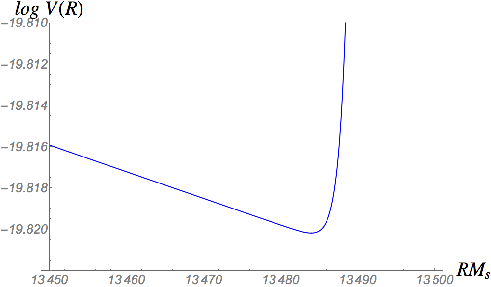
As promised the minimum is automatically balanced to appear at the correct values of $R_{min}$. An example of the potential is shown in fig. 1 for sample values. It is essentially a $1/R^{4}$ runaway to large radius until the ISS contribution takes over where the SQCD gauge coupling is starting to become strong. The minimum is de Sitter, and of order $10^{-3}M_{KK}^{4}$. Clearly for consistency one would then require some additional $R$-independent and negative contribution to bring the final cosmological constant close to zero.

Note that going along implicitly with need to protect the ISS mechanism from the supersymmetry breaking of the SS mechanism, is of course the converse assumption that the effects of strong coupling in the SCQD sector do not disrupt the original calculation of the Casimir energy. This assumption is credible because the latter is dominated by the tower of KK states with masses between $M_{KK}$ and $M_{s}$, and above physics occurring at the scale $\Lambda_{e}$ provided that the $\Lambda_{e}<1/R_{min}$ constraint is satisfied. This condition can be relaxed in various cases and under various assumptions which will be made more precise when we come to study the string embedding in later sections.

The form of the potential for $R\gg R_{min}$ is not well determined. In these regions the dynamical scale is larger than the KK scale (i.e. $R\Lambda_{e}(R)\gg 1$) so the sufficient condition in eq.(3) is violated. Most probably this implies that the potential turns over at some point, and the minimum at $R_{min}$ is metastable in the $R$ direction as well, with larger values simply reverting to runaway behaviour. It is not clear how the large radius limit of such theories lifts to the decompactified 6D theory; most likely it is related to the 4D IR free magnetic dual of the ISS theory, rather than the original electric SQCD theory.

If one makes the conservative assumption that the minimum derived above is indeed only metastable, it is important to consider what the tunnelling rate would be to continued runaway along $R$, in order to confirm that it is sufficiently small. An estimate requires the normalization of the modulus corresponding to $R$. In flat space compactifications derived from string theory the Kähler potential is given by $K\sim-\log V$ where $V$ is the overall compactification volume. In the present case one can identify $V\sim i\left(T_{R}-\bar{T}_{R}\right)$ with $T_{R}$ being a holomorphic modulus whose imaginary part gives $R$. This would give kinetic terms for $R$ of the form $\mathcal{L}\supset\frac{|\partial T_{R}|^{2}}{R^{2}}$ so the canonically normalised field is $\phi_{R}=T_{R}/R_{min}$. The tunnelling action can then be approximated in the thick wall limit. The advantage of this physical situation is that the height of the barrier does not appear in the action at leading order, only its width and the difference $\Delta V$ between the vacuum energies of the false and true minima. A crude estimate for the action is then [43]

$$S_{E}\sim 2\pi^{2}\frac{\left(\Delta\phi_{R}\right)^{4}}{\Delta V}\,,$$

(19)

where $\Delta V=V_{false}-V_{true}=R_{min}^{-4}\alpha_{D}^{2}N\left(R_{min}\Lambda_{e}\right)^{2}$. As this is a sufficient condition, let us adopt a conservative value for $\Delta\phi_{R}$, namely the distance in field-space between $R_{min}$ and the point where perturbativity breaks down, $\Lambda_{e}R\sim 1$, or $\frac{\Lambda_{e}R_{min}}{\Lambda_{e}R}=\mu_{0}/M_{s}=e^{-\frac{C}{b}\Delta RM_{s}}$. This gives

$$\Delta\phi_{R}\approx R_{min}^{-1}\frac{b}{C}\log\frac{M_{s}}{\mu_{0}}\,,$$

(20)

leading to an estimate for the tunnelling action of

$$S_{E}\sim\frac{2\pi^{2}}{\alpha^{2}}\left(\frac{M_{s}}{\mu_{0}}\right)^{2}\sim 10^{3}/\alpha^{2}.$$

(21)

This is well above the $S_{E}\gtrsim 400$ that is required to ensure stability on timescales of the age of the universe (see e.g. ref. [44] and references therein). Heuristically this is simply a consequence of the fact that the Casimir energy in $V$ is a one-loop effect (given by $\rho$), so the potential is much flatter than it is broad.

Models that are non-supersymmetric but nevertheless have equal numbers of massless bosons and fermions $(N_{f}^{0}=N_{b}^{0})$ have a one-loop cosmological constant that is exponentially suppressed. Ref. [13] argues that these cases are particularly interesting due to their enhanced stability properties, and form a better basis for doing phenomenology.

The philosophy in these cases is somewhat different: the general idea is that the exponential suppression appearing in the vacuum energy also appears in the scale setting the Higgs mass. Therefore the compactification volume (and consequently the SS supersymmetry breaking scale $1/R$) needs to be only so large so as to be able to generate the necessary suppression, while it is possible to live with supersymmetry breaking that is much larger than the electroweak scale (the canonical situation with SS breaking). The issue for the present discussion then is how to stabilise with exponentially small cosmological constant and reasonable coupling, but still with moderately large volume.

As already mentioned, the aspect of these theories that will be of particular relevance is that the only modes that make a non-vanishing contribution to the vacuum energy have string sized masses, and indeed the leading contribution to the Schwinger integral comes from a saddle-point at the UV end, $t\sim 1$, rather than from the entire integral, as is the case for a generic theory. Consequently the contribution to the cosmological constant resulting from the Scherk-Schwarz mechanism is blind to the IR physics occurring in for example the ISS mechanism, and the two contributions are physically separated. Indeed the former cannot easily be understood within an effective field theory²² 2 Conceivably one could try to write down a supergravity theory truncated at the first string excitation level..

As already mentioned, to emphasise the distinction these theories will be said (using the terminology in its broad sense) to have a UV-Casimir energy. An additional advantage in the present context is of course that the volumes required are much smaller than the generic case, and hence the decompactification problem is less pronounced.

Assuming that the exponential suppression continues beyond one-loop, such cases have to be treated quite differently. In the present toy model, the ISS mechanism essentially governs the minimisation, and the issue is to ensure that the contribution to the cosmological constant from the initial SS mechanism is negligible. The 5D case is as follows.

First let us return to the constraints in eq.(3). The potential takes the form

$$V=R^{-4}\left[\alpha^{2}\rho(N_{f}^{1}-N_{b}^{1})(RM_{s})^{2}e^{-4\pi RM_{s}}+N_{c}\alpha_{D}^{2}(R\Lambda_{e})^{2}\right]\,,$$

(22)

where $N_{f}^{1}-N_{b}^{1}$ counts the fermi-bose non-degeneracy at the first excited string level, $\alpha$ stands again for a generic Scherk-Schwarz phase, while $\rho\ll 1$ is now generically a one-loop suppression factor. As is evident from eq.(14) the SS term dies away rapidly at large radius. The minimum occurs shortly after the second term has its independent minimum at

$\displaystyle R_{min}M_{s}$

$\displaystyle=$

$\displaystyle\frac{4b}{C}\,,$

(23)

so the string scale can be perhaps an order of magnitude higher than the KK scale. It is useful to define $\sigma\gtrsim 0$ as the final ratio of dynamical to KK scale, i.e. $R_{min}\Lambda_{e}=e^{-\sigma}$, so that ultimately

$$\sigma=\frac{8\pi^{2}}{|b|g_{s}^{2}}-2\,.$$

(24)

As usual, $m_{D}$ must satisfy the constraints in eq.(3), so it lies below $\Lambda_{e}$ but is large enough that $\hat{m}_{D}\Lambda_{e}>\alpha^{2}/R^{2}$:

$\displaystyle 1\gtrsim e^{-\frac{8\pi^{2}}{|b|g_{s}^{2}}+2}$

$\displaystyle\gg$

$\displaystyle\alpha_{D},\,\alpha^{2}/\alpha_{D}\,.$

(25)

Thus for the mechanism to work when the Casimir energy is exponentially suppressed in the 5D$\rightarrow$4D theory, the scale of supersymmetry breaking has to be at most a few orders of magnitude below the string scale with relatively large coupling, $8\pi^{2}/|b|g_{s}^{2}\sim 2$. In addition $\alpha_{D}\sim\alpha$ are required to be small. Note that if these constraints are satisfied then the SS contribution to the cosmological constant is guaranteed to be negligible at the minimum, which was the point we wished to demonstrate here. The essential advantage of a UV-Casimir energy in this case is that the (relatively) large volume stabilisation governed by non-perturbative long-range physics has not fed-back into it, so one has the sort of modularity normally associated with brane configurations.

As an example, taking $|C|=10$, $|b|=30$, $g_{s}=1/\sqrt{2}$, one requires $\alpha,\alpha_{D}\lesssim R\Lambda_{e}\approx 1/25$. We will later see how to accommodate $\Lambda_{e}>M_{KK}$ in the 6D$\rightarrow$4D version; this removes the upper bound in eq.(25) allowing maximal SS phases $\alpha_{D},\alpha\sim 1$.

First let us establish how the Scherk-Schwarz mechanism in a direct string implementation such as that in ref. [13] maps to the effective supergravity theory. As mentioned, the SS stage of compactification is on an orbifolded $\mathbb{T}_{2}$ torus, which in the absence of Wilson lines can be described generally by the metric

$$G_{ij}=\frac{T_{2}}{U_{2}}\left(\begin{array}[]{cc}1&U_{1}\\ U_{1}&|U|^{2}\end{array}\right)\,\,\,;\,\,\,\,G^{ij}=\frac{1}{T_{2}U_{2}}\left(\begin{array}[]{cc}|U|^{2}&-U_{1}\\ -U_{1}&1\end{array}\right)\,,$$

(26)

where in order to conform with most of the phenomenology oriented SUGRA literature the convention is

	$\displaystyle iU$	$\displaystyle=$	$\displaystyle U_{1}+iU_{2}$
	$\displaystyle iT$	$\displaystyle=$	$\displaystyle T_{1}+iT_{2}\,.$		(27)

For reference, untilted tori have $U_{1}=0$, $T_{2}=R_{1}R_{2}$, $U_{2}=R_{2}/R_{1}$ where $R_{i}$ is the radius along direction $i$, and it will be assumed throughout that $R_{2}>R_{1}$. The $U_{1}$ modulus encapsulates the tilt angle (i.e. $U_{1}=R_{2}\cos\theta/R_{1}$, $U_{2}=R_{2}\sin\theta/R_{1}$) and $T_{2}=R_{1}R_{2}\sin\theta$ is the volume. The nett effect on the spectrum of the Scherk-Schwarz action can be determined on the string theory side from the shift in the internal momenta, which can in turn be read off the partition function. The latter contains a factor

$$\mathcal{Z}_{d,d}(G,B)=\frac{1}{|\eta(\tau)|^{2d}}\sum_{\mathbf{n},\mathbf{m}}q^{\alpha^{\prime}\mathbf{p_{L}^{2}/2}}\bar{q}^{\alpha^{\prime}\mathbf{p_{R}^{2}/2}},$$

(28)

coming from the compactified toroidal directions. The momenta depend on the KK numbers $m_{1,2}$ and winding numbers $n^{1,2}$ of the $\mathbb{T}_{2}$ as

	$\displaystyle\mathbf{p}_{L}^{2}$	$\displaystyle=$	$\displaystyle p_{L_{i}}G^{ij}p_{L_{j}}$
	$\displaystyle p_{L_{j}}$	$\displaystyle=$	$\displaystyle\frac{1}{\sqrt{2\alpha^{\prime}}}\left(m_{j}+(B_{jk}+G_{jk})n^{k}\right)\,,$		(29)

and

	$\displaystyle\mathbf{p}_{R}^{2}$	$\displaystyle=$	$\displaystyle p_{R_{i}}G^{ij}p_{R_{j}}$
	$\displaystyle p_{Rj}$	$\displaystyle=$	$\displaystyle\frac{1}{\sqrt{2\alpha^{\prime}}}\left(m_{j}+(B_{jk}-G_{jk})n^{k}\right)\,,$		(30)

where the notation throughout is as in ref. [13]. The Scherk-Schwarz action causes a discrete Lorentz rotation and boost involving the KK and winding numbers and the charge/momentum lattice, $\mathbf{Q}$, of the form

	$\displaystyle\mathbf{Q}$	$\displaystyle\rightarrow$	$\displaystyle\mathbf{Q}-n^{i}\mathbf{e}_{i}$
	$\displaystyle m_{i}$	$\displaystyle\rightarrow$	$\displaystyle m_{i}+\mathbf{Q}\cdot\mathbf{e}_{i}-\frac{1}{2}\mathbf{e}_{i}\cdot\mathbf{e}_{j}n^{j}$
	$\displaystyle B_{jk}\pm G_{jk}$	$\displaystyle\rightarrow$	$\displaystyle B_{jk}\pm G_{jk}-\frac{1}{4}\mathbf{e}_{j}\cdot\mathbf{e}_{k}\,\,\,,$		(31)

where $\mathbf{e}_{i=1,2}$ are vectors containing the Scherk-Schwarz action on the $R$-charges and possibly also gauge charges, and the dot product refers to the Lorentzian charge lattice. The vectors $\mathbf{e}_{i}$ contain the phases $\alpha_{F,B}$, although one should note they must leave the world sheet supercurrent and charge lattice invariant, and have to leave a consistent orbifold projection. It is for these reasons that $\alpha_{F,B}$ are constrained to be discrete.

Specialising to the maximal twist case, the spontaneous supersymmetry breaking arises from half integer values of the $\mathbf{Q}\cdot\mathbf{e}_{i}$ shift in the KK numbers. Consider the gravitinos; adding left and right moving contributions, the modes $m_{i}$ and $\mathbf{Q}\cdot\mathbf{e}_{i}$ marry with the modes $-m$ and $-\mathbf{Q}\cdot\mathbf{e}_{i}$, so that

	$\displaystyle\left(m_{3/2}^{(m_{1}m_{2})}\right)^{2}$	$\displaystyle=$	$\displaystyle\frac{1}{\alpha^{\prime}}\hat{m}_{i}G^{ij}\hat{m}_{j}=\frac{1}{4\alpha^{\prime}}\sum_{ij}G^{ij}$		(32)
		$\displaystyle=$	$\displaystyle\frac{1}{\alpha^{\prime}}\frac{1}{T_{2}U_{2}}\left|(m_{1}-\frac{1}{2})-(m_{2}-\frac{1}{2})iU\right|^{2}\,.$

Clearly supersymmetry is restored for all $U_{1}=\frac{2\ell_{1}-1}{2\ell_{2}-1}$ in the limit $U_{2}\rightarrow 0$ for integer $\ell_{1,2}$. This limit can be achieved by decompactifying with constant ratio of radii, with the tilt angle going to zero (slower than $1/R_{1}R_{2}$ in order for $T_{2}$ to go to large volume). An identical mass-shift is induced in the gauginos. From this we can identify the effective KK scale near a supersymmetric point as $M_{KK}^{2}=U_{2}/T_{2}=1/R_{1}^{2}$. (Where necessary factors of $\alpha^{\prime}$ are absorbed into the modulus $T$ to give it dimensions of length squared.)

Continuous Wilson lines shift the KK and winding numbers along with the internal charges in a similar fashion and these can be related to matter/Higgs fields: the shift induced by the pair of continuous real Wilson lines $\mathbf{A}_{1}$, $\mathbf{A}_{2}$, can be written

	$\displaystyle\mathbf{Q}$	$\displaystyle\rightarrow$	$\displaystyle\mathbf{Q}+n^{i}\mathbf{A}_{i}$
	$\displaystyle m_{i}$	$\displaystyle\rightarrow$	$\displaystyle m_{i}-\mathbf{Q}\cdot\mathbf{A}_{i}$
	$\displaystyle B_{jk}\pm G_{jk}$	$\displaystyle\rightarrow$	$\displaystyle B_{jk}\pm G_{jk}-\frac{1}{4}\mathbf{A}_{j}\cdot\mathbf{A}_{k}\,\,\,.$		(33)

The real shift vectors $\mathbf{A}_{i}$ can be related to a pair of complex fields in the effective supergravity theory, denoted $\phi$, $\phi^{\prime}$. To get to this basis, first define complex Wilson lines,

$$\mathbf{Z}=iU\mathbf{A}_{1}-\mathbf{A}_{2}\,,$$

(34)

and then

	$\displaystyle i\phi$	$\displaystyle=$	$\displaystyle\frac{1}{2}(Z^{1}-iZ^{2})$
	$\displaystyle i\phi^{\prime}$	$\displaystyle=$	$\displaystyle\frac{1}{2}(Z^{1}+iZ^{2})\,.$		(35)

The upper indices refer to basis vectors for the charge lattice. Defining $2P=\phi+\bar{\phi^{\prime}}$, useful combinations are (in our conventions)

	$\displaystyle P\bar{P}$	$\displaystyle=$	$\displaystyle\sum_{a}\Im(Z^{a})^{2}=\left(\mathbf{A}_{1}\cdot\mathbf{A}_{1}\right)\frac{U_{2}^{2}}{4}$
	$\displaystyle T_{2}$	$\displaystyle=$	$\displaystyle\sqrt{G}+P\bar{P}/U_{2}$
	$\displaystyle U$	$\displaystyle=$	$\displaystyle\frac{1}{G_{11}}\left(\sqrt{G}-iG_{12}\right)\,,$		(36)

with the $T_{2}$ redefinition matching the shift in (33). Going from $\mathbf{Z}$ to $\phi$, $\phi^{\prime}$ amounts to a change of basis for $\mathbf{Q}$. For example the current superfield for a $U(1)$ current (under which $\phi$ and $\phi^{\prime}$ must have opposite charges) is given by, $J=|\phi|^{2}-|\phi^{\prime}|^{2}=\frac{i}{2}\left(Z^{1}\bar{Z}^{2}-Z^{2}\bar{Z}^{1}\right)$, so its generator acts as $SO(2)$ on the $Z^{a}$ indices. The Kähler potential depends on the volume $\sqrt{G}$ as

$$K=-\log Y-\log 4(T_{2}U_{2}-P\bar{P})\,,$$

(37)

where $2P=\phi+\bar{\phi^{\prime}}$, and where the dilaton combination generally includes a term from the (heterotic) Green-Schwarz mechanism,

$$Y=S+\bar{S}-\delta_{GS}\log 4(T_{2}U_{2}-P\bar{P})\,.$$

(38)

So far the picture is just that of the standard $\mathcal{N}=1$ theories, but now we deform the theory with a superpotential that successfully reproduces the SSSB observed in the string spectrum. As we saw on the string side in eq.(32), near $iU=1$ the lightest spin 3/2 state is the zero-KK mode gravitino whose physical mass is

$$m_{3/2}^{2}=\frac{1}{4}\frac{1}{S_{2}T_{2}U_{2}}|1-iU|^{2}.$$

(39)

The relation between the Planck scale and string scale is

$$M_{P}^{2}=g_{s}^{-2}\alpha^{\prime-1}\,,$$

(40)

which suggests that a superpotential in the spontaneously broken theory that produces the correct spectrum is

$$W_{SS}=\sqrt{2}(1-iU)\,.$$

(41)

It can be verified that near $U_{1}=1$, the rest of the low-lying tree-level string spectrum is successfully generated by this supergravity theory. Explicitly, in the string spectrum the tree-level gaugino masses are degenerate with the gravitino: using standard notation, the supercovariant derivative is $D_{i}W=W_{i}+WK_{i}$, and the gauge kinetic function is $f_{tree}=S$, leading to

$$m_{\lambda}=\left|\frac{m_{3/2}}{2}Re(f_{tree})^{-1}K^{\bar{i}j}\partial_{i}f_{tree}\frac{D_{\bar{j}}\bar{W}}{\bar{W}}\right|=m_{3/2}\,.$$

(42)

At one-loop the masses would not be equal in either the field theory or the string theory due to gauge mediation effects, but we shall see below that the above relation does not suffer large volume corrections.

Continuing the comparison of the spectra, after spontaneous superymmetry breaking all the untwisted scalars in the NS-NS sector should remain massless at tree-level, while their fermion superpartners pick up a mass equal to that of the gravitino. The corresponding superfields, $\phi$ and $\phi^{\prime}$, achieve this by appearing to conspire in the Kähler potential as

	$\displaystyle K$	$\displaystyle\supset$	$\displaystyle-\log\left(4T_{2}U_{2}-|\phi+\bar{\phi^{\prime}}|^{2}\right)$		(43)
		$\displaystyle=$	$\displaystyle-\log 4T_{2}U_{2}+\frac{1}{4T_{2}U_{2}}(|\phi|^{2}+|\phi^{\prime}|^{2}+\phi\phi^{\prime}+\bar{\phi}\bar{\phi^{\prime}})+\ldots$

The tree-level fermion mass terms in the effective theory (which is a “$\mu$-term” if one is thinking of $\phi$,$\phi^{\prime}$ as Higgses), are then given by

$$\mu_{\phi}=m_{3/2}Z_{\phi}^{-\frac{1}{2}}Z_{\phi^{\prime}}^{-\frac{1}{2}}\left(\frac{W_{ij}}{W}+K_{ij}-\Gamma_{ij}^{k}\frac{D_{k}W}{W}\right)\,,$$

(44)

where

	$\displaystyle\Gamma_{ij}^{k}$	$\displaystyle=$	$\displaystyle K^{k\bar{k}}\partial_{\bar{k}}K_{ij}$
	$\displaystyle Z_{\phi}^{-1}=Z_{\phi^{\prime}}^{-1}$	$\displaystyle=$	$\displaystyle 4T_{2}U_{2}=1/K_{\phi\phi^{\prime}}\,.$		(45)

Inserting the supersymmetry breaking superpotential in eq.(41) gives

$$\mu_{\phi}=m_{3/2}\left(4T_{2}U_{2}\frac{W_{ij}}{W}-\frac{\bar{W}}{W}\right)\,.$$

(46)

In the absence of any explicit $W_{ij}$ mass terms in the original superpotential, this automatically has the same magnitude as the gaugino and gravitino masses in accord with the Scherk-Schwarzed string theory spectrum. It is straightforward to show that $S,U,T,\phi$ and $\phi^{\prime}$ fit into a larger “no-scale” supergravity structure that leaves all the scalars massless at tree-level (modulo possible variations in the splittings of the matter fields that may arise if $\mathbf{e}$ is also embedded into the gauge groups: in the effective theory this would correspond to turning on scalar “Higgs” VEVs). The conspiring dimensionful terms correspond to mass-squareds and Dirac masses of magnitude $m_{3/2}$ for the canonically normalized states.

The original ${\cal N}=1$ theory has well-known modular symmetries: for completeness the standard $SL(2,\mathbb{Z})_{T}$ and $SL(2,\mathbb{Z})_{U}$ symmetries of the supersymmetric theory are included in the Appendix. What remains of them after applying the Scherk-Schwarz mechanism? Due to the spontaneous nature of the breaking it is clear that the Kähler potential should still respect the full symmetry, as it indeed does, and that the new SSSB superpotential should be the only source of its breaking. To see its effect on the modular symmetries consider the spectrum: according to eq.(32) the zero-mode KK gravitino need not be the lightest state, depending on the value of $U_{1}$. If $U_{1}=\frac{2\ell_{1}-1}{2\ell_{2}-1}$ then the lightest gravitino is instead the $\ell_{1},\ell_{2}$ KK mode for all $U_{2}\lesssim 1/(2\ell_{2}+1)$, and the superpotential in the effective theory would actually be $W_{SS}=\sqrt{2}((2\ell_{1}-1)-(2\ell_{2}-1)iU)$ near this point. The fact that one has to specify which mode plays the role of the gravitino in the effective theory is of course just a symptom of the deficiency of the 4D supergravity approximation, which cannot describe the supersymmetry breaking over the whole $U$ moduli-space. Indeed the explicit breaking of modular symmetry in the superpotential just amounts to a choice of gauge: because of the original discrete symmetry, there are infinitely many equivalent spontaneously broken theories that one could write down for the effective supergravity theory related by a subgroup of the $SL(2,\mathbb{Z})_{U}$ transformations. This is evident from the fact that under transformations of the form

$$\frac{1}{4}\frac{|1-iU|^{2}}{S_{2}T_{2}U_{2}}\equiv\frac{1}{4}\frac{|(d-b)-(a-c)iU|^{2}}{S_{2}T_{2}U_{2}}\,\,\,;\,\,a,b,c,d\in\mathbb{Z},\,\,ad-bc=1,\,\,a-c=b-d=1\,\mbox{mod}(1)\,,$$

(47)

the gravitino spectrum is invariant. In fact the entire theory is invariant only under the smaller congruence subgroup defined by $a,d=1$ mod (1) and $b,c=0$ mod (1), similar to ref. [33], which will be referred to as $\Gamma_{\vartheta}(2)$. Under such transformations, any $U$ in a maximally twisted Scherk-Schwarz theory can be mapped to the fundamental domain shown in fig. 2. In addition to the cusp at infinity, there is a single representative supersymmetric cusp at $iU=1$. For non-maximal Scherk-Schwarz twists, the fundamental domain will contain more cusps, and there will be several genuinely distinct supersymmetric vacua (consult ref. [33] for details). Naturally the Casimir energy, when we come to calculate it, must respect this symmetry.

We will also need an understanding of the one-loop gauge thresholds. Their volume dependence (neglecting the effects of extra charged massless states) can be written [33]

$$\Delta=-C\log\left(T_{2}U_{2}|\eta(iT)|^{4}|\eta(iU)|^{4}\right)+(C-b)\log\left(T_{2}U_{2}|\vartheta_{4}(iT)|^{4}|\vartheta_{2}(iU)|^{4}\right)\,,$$

(48)

where $b=16\pi^{2}\beta$ is the beta function coefficients for the entire massless theory, $C=16\pi^{2}\beta_{\mathcal{N}=2}$ is the $N=2$ coefficient, and $\eta$ are the usual Dedekind eta functions. The modular functions in this expression are also invariant under $\Gamma_{\vartheta}(2)$ transformations; denoting $SL(2,\mathbb{Z})_{U}$ operations by $S_{U}\equiv iU\rightarrow-1/iU$ and $T_{U}\equiv iU\rightarrow iU+1$, we have

	$\displaystyle T_{U}:U_{2}|\vartheta_{2}(iU)|^{4}$	$\displaystyle\longrightarrow$	$\displaystyle U_{2}|\vartheta_{2}(iU)|^{4}$		(49)
	$\displaystyle S_{U}:U_{2}|\vartheta_{2,4}(iU)|^{4}$	$\displaystyle\longrightarrow$	$\displaystyle U_{2}|\vartheta_{4,2}(iU)|^{4}\,.$		(50)

Therefore $\Delta$ is invariant under any number of $T_{U}$ moves, but only an even number of $S_{U}$ moves, in accord with the congruence condition.

Following now the standard route (see for example refs. [47, 48, 49, 50]) this allows us to identify the holomorphic gauge kinetic function of the SQCD as (taking a Kac-Moody level $k=1$ for the gauge group),

$$f=S-\frac{C}{8\pi^{2}}\log\eta(iT)^{2}\eta(iU)^{2}+\frac{C-b}{8\pi^{2}}\log\left(\vartheta_{4}(iT)^{2}\vartheta_{2}(iU)^{2}\right)\,,$$

(51)

with the gauge coupling being given by

$$\frac{2}{g^{2}}=Y=2\Re(f)-\frac{b}{8\pi^{2}}\log(\mu^{2})-\left(\frac{b}{8\pi^{2}}+\delta_{GS}\right)\log(4T_{2}U_{2})\,.$$

(52)

Note that due to the additional universal terms it is the $\mathcal{N}=1$ beta function appearing here (i.e. $b=-3N+F$ in $SU(N)$ gauge theories with $\mathcal{N}=1$ SQCD and $F$ flavours), and not $C$.

The holomorphic dynamical scale $\Lambda_{hol}$ can be defined as

$$\Lambda_{hol}=\exp\left(-\frac{8\pi^{2}}{|b|}f\right)\,,$$

(53)

and the modular weight of $\Lambda_{hol}$ is given by

$$n_{\Lambda}=8\pi^{2}\frac{b/8\pi^{2}+\delta_{GS}}{|b|}\,.$$

(54)

The gauge coupling can then be written more succinctly as

$$\frac{1}{g^{2}(\mu)}=-\frac{b}{8\pi^{2}}\log\left[\frac{\mu}{|\Lambda_{hol}|(4T_{2}U_{2})^{n_{\Lambda}/2}}\right]\,.$$

(55)

It will often be useful to leave $n_{\Lambda}$ implicit, as it is essentially just whatever combination of terms appears in eq.(52). However it can be calculated directly [48]; specialising to $SU(N)$ gauge theories with $\mathcal{N}=1$ SQCD and $F$ flavours of quark and anti-quark, it is

$$|b|n_{\Lambda}=2Fn_{Q}+F-N\,.$$

(56)

We will see that this equation provides an important consistency condition for the implementation of the ISS mechanism, because it can be derived independently from the matching conditions for the Seiberg duals. Note that it will be assumed for simplicity throughout that the $SL(2,\mathbb{Z})_{U}$ and $SL(2,\mathbb{Z})_{T}$ weights are degenerate for every field.

To complete this part of the discussion, one can obtain an asymptotic approximation for the gauge threshold correction at large volume and in the supersymmetric limit around the representative cusp at $iU=1$ (which obviously breaks the modular symmetry). In the vicinity of the cusp, since $\lim_{iU\rightarrow 1}\eta(iU)=0$, it is often convenient to use $SL(2,\mathbb{Z})_{U}$ modular redefinitions to the cusp at infinity, that is $i\tilde{U}=-1/(iU-1)\approx i/U_{2}$, with $i\tilde{U}\rightarrow i\infty$ in the supersymmetric limit: the standard expansion $\vartheta_{4}(i\tilde{U})\rightarrow 1-2e^{-\pi\tilde{U}}+\ldots$ then gives,

	$\displaystyle\Delta$	$\displaystyle=$	$\displaystyle-C\log\left(4T_{2}\tilde{U}_{2}|\eta(iT)|^{4}|\eta(i\tilde{U})|^{4}\right)+(C-b)\log\left(4T_{2}\tilde{U}_{2}|\vartheta_{4}(iT)|^{4}|\vartheta_{4}(i\tilde{U})|^{4}\right)\,,$		(57)
		$\displaystyle=$	$\displaystyle\frac{\pi}{3}C\left(T_{2}+\tilde{U}_{2}\right)-b\log\left(4T_{2}\tilde{U}_{2}\right)+\mathcal{O}(e^{-\pi\tilde{U}_{2}},e^{-\pi T_{2}})\,.$

As in the 5D case, the second term subtracts from $16\pi^{2}/g(\mu)^{2}$ the logarithmic running between the lightest KK-mode $M_{KK}=1/\sqrt{4T_{2}\tilde{U}_{2}}$ and the string scale, whilst the first term replaces it with a power-law threshold. Under our assumption that $C/b>0$, it is clear that one is prevented from going continuously to the boundary of moduli-space by the appearance of strong coupling in the QCD theory where $\frac{\pi}{3}C\left(T_{2}+\tilde{U}_{2}\right)\sim 16\pi^{2}$, and this is precisely the region in which the minimum is expected to appear.

References

- [1] J. Scherk and J. H. Schwarz, “Spontaneous Breaking of Supersymmetry Through Dimensional Reduction,” Phys. Lett. B 82, 60 (1979). doi:10.1016/0370-2693(79)90425-8
- [2] J. Scherk and J. H. Schwarz, “How to Get Masses from Extra Dimensions,” Nucl. Phys. B 153, 61 (1979). doi:10.1016/0550-3213(79)90592-3
- [3] I. Antoniadis, “A Possible new dimension at a few TeV,” Phys. Lett. B 246, 377 (1990). doi:10.1016/0370-2693(90)90617-F
- [4] I. Antoniadis, K. S. Narain and T. R. Taylor, “Higher genus string corrections to gauge couplings,” Phys. Lett. B 267, 37 (1991). doi:10.1016/0370-2693(91)90521-Q
- [5] I. Antoniadis, S. Dimopoulos, A. Pomarol and M. Quiros, “Soft masses in theories with supersymmetry breaking by TeV compactification,” Nucl. Phys. B 544, 503 (1999) doi:10.1016/S0550-3213(99)00037-1 [hep-ph/9810410].
- [6] D. M. Ghilencea, H. P. Nilles and S. Stieberger, “Divergences in Kaluza-Klein models and their string regularization,” New J. Phys. 4 (2002) 15 doi:10.1088/1367-2630/4/1/315 [hep-th/0108183].
- [7] S. Dimopoulos, K. Howe and J. March-Russell, “Maximally Natural Supersymmetry,” Phys. Rev. Lett. 113, 111802 (2014) doi:10.1103/PhysRevLett.113.111802 [arXiv:1404.7554 [hep-ph]].
- [8] T. Cohen, N. Craig, H. K. Lou and D. Pinner, “Folded Supersymmetry with a Twist,” JHEP 1603, 196 (2016) doi:10.1007/JHEP03(2016)196 [arXiv:1508.05396 [hep-ph]].
- [9] I. Garcia Garcia, K. Howe and J. March-Russell, “Natural Scherk-Schwarz Theories of the Weak Scale,” JHEP 1512, 005 (2015) doi:10.1007/JHEP12(2015)005 [arXiv:1510.07045 [hep-ph]].
- [10] K. Tobioka, R. Kitano and H. Murayama, “Enhanced Higgs Mass in Compact Supersymmetry,” JHEP 1604, 025 (2016) doi:10.1007/JHEP04(2016)025 [arXiv:1511.04081 [hep-ph]].
- [11] I. Antoniadis, K. Benakli and M. Quiros, “Sequestered gravity in gauge mediation,” Eur. Phys. J. C 76, no. 7, 363 (2016), [arXiv:1512.00029 [hep-ph]].
- [12] M. Reece and W. Xue, “SUSY?s Ladder: reframing sequestering at Large Volume,” JHEP 1604, 045 (2016) doi:10.1007/JHEP04(2016)045 [arXiv:1512.04941 [hep-ph]].
- [13] S. Abel, K. R. Dienes and E. Mavroudi, “Towards a nonsupersymmetric string phenomenology,” Phys. Rev. D 91, no. 12, 126014 (2015) doi:10.1103/PhysRevD.91.126014 [arXiv:1502.03087 [hep-th]].
- [14] E. Ponton and E. Poppitz, “Casimir energy and radius stabilization in five-dimensional orbifolds and six-dimensional orbifolds”, JHEP 0106 (2001) 019, [hep-ph/0105021].
- [15] M. Borunda, M. Serone and M. Trapletti, “On the quantum stability of IIB orbifolds and orientifolds with Scherk-Schwarz SUSY breaking,” Nucl. Phys. B 653, 85 (2003) doi:10.1016/S0550-3213(03)00040-3 [hep-th/0210075].
- [16] G. von Gersdorff, M. Quiros and A. Riotto, “Scherk-Schwarz supersymmetry breaking with radion stabilization,” Nucl. Phys. B 689, 76 (2004) doi:10.1016/j.nuclphysb.2004.04.010 [hep-th/0310190].
- [17] E. Dudas and C. Timirgaziu, “Nontachyonic Scherk-Schwarz compactifications, cosmology and moduli stabilization,” JHEP 0403, 060 (2004) doi:10.1088/1126-6708/2004/03/060 [hep-th/0401201].
- [18] E. Dudas and M. Quiros, “Five-dimensional massive vector fields and radion stabilization,” Nucl. Phys. B 721, 309 (2005) doi:10.1016/j.nuclphysb.2005.05.028 [hep-th/0503157].
- [19] G. von Gersdorff and A. Hebecker, “Radius stabilization by two-loop Casimir energy,” Nucl. Phys. B 720, 211 (2005) doi:10.1016/j.nuclphysb.2005.06.001 [hep-th/0504002].
- [20] C. Angelantonj, M. Cardella and N. Irges, “An Alternative for Moduli Stabilisation,” Phys. Lett. B 641, 474 (2006) doi:10.1016/j.physletb.2006.08.072 [hep-th/0608022].
- [21] A. P. Braun, A. Hebecker and M. Trapletti, “Moduli stabilization in (string) model building: Gauge fluxes and loops,” arXiv:0710.4877 [hep-th].
- [22] C. Gross and A. Hebecker, “A Realistic Unified Gauge Coupling from the Micro-Landscape of Orbifold GUTs,” Nucl. Phys. B 821, 354 (2009) doi:10.1016/j.nuclphysb.2009.06.030 [arXiv:0812.4267 [hep-ph]].
- [23] K. R. Dienes, E. Dudas and T. Gherghetta, “Extra space-time dimensions and unification,” Phys. Lett. B 436, 55 (1998) [hep-ph/9803466]; “Grand unification at intermediate mass scales through extra dimensions,” Nucl. Phys. B 537, 47 (1999) [hep-ph/9806292]; “TeV scale GUTs,” hep-ph/9807522.
- [24] K. R. Dienes, E. Dudas and T. Gherghetta, “GUT precursors and nontrivial fixed points in higher dimensional gauge theories,” Phys. Rev. Lett. 91, 061601 (2003) [hep-th/0210294]; “GUT precursors and fixed points in higher-dimensional theories,” Pramana 62, 219 (2004).
- [25] E. Caceres, V. S. Kaplunovsky and I. M. Mandelberg, “Large volume string compactifications, revisited,” Nucl. Phys. B 493, 73 (1997) doi:10.1016/S0550-3213(97)00129-6 [hep-th/9606036].
- [26] E. Kiritsis, C. Kounnas, P. M. Petropoulos and J. Rizos, “Solving the decompactification problem in string theory,” Phys. Lett. B 385 (1996) 87 [hep-th/9606087].
- [27] E. Kiritsis, C. Kounnas, P. M. Petropoulos and J. Rizos, “String threshold corrections in models with spontaneously broken supersymmetry,” Nucl. Phys. B 540, 87 (1999) [hep-th/9807067].
- [28] I. Antoniadis and K. Benakli, “Large dimensions and string physics in future colliders,” Int. J. Mod. Phys. A 15, 4237 (2000) [hep-ph/0007226].
- [29] A. E. Faraggi, C. Kounnas and H. Partouche, “Large volume susy breaking with a solution to the decompactification problem,” Nucl. Phys. B 899, 328 (2015) doi:10.1016/j.nuclphysb.2015.08.001 [arXiv:1410.6147 [hep-th]].
- [30] C. Kounnas and H. Partouche, “Stringy N = 1 super no-scale models,” PoS PLANCK 2015, 070 (2015) [arXiv:1511.02709 [hep-th]].
- [31] C. Kounnas and H. Partouche, “Super no-scale models in string theory,” arXiv:1607.01767 [hep-th].
- [32] H. Partouche, “Large volume supersymmetry breaking without decompactification problem,” arXiv:1601.04564 [hep-th].
- [33] C. Angelantonj, I. Florakis and M. Tsulaia, “Generalised universality of gauge thresholds in heterotic vacua with and without supersymmetry,” Nucl. Phys. B 900, 170 (2015) doi:10.1016/j.nuclphysb.2015.09.007 [arXiv:1509.00027 [hep-th]].
- [34] K. A. Intriligator, N. Seiberg and D. Shih, “Dynamical SUSY breaking in meta-stable vacua,” JHEP 0604, 021 (2006) doi:10.1088/1126-6708/2006/04/021 [hep-th/0602239].
- [35] R. Rohm, “Spontaneous Supersymmetry Breaking in Supersymmetric String Theories,” Nucl. Phys. B 237, 553 (1984).
- [36] S. Ferrara, C. Kounnas and M. Porrati, “ Superstrings With Spontaneously Broken Symmetries,” Phys. Lett. B 206, 25 (1988).
- [37] S. Ferrara, C. Kounnas and M. Porrati, “Superstring Solutions With Spontaneously Broken Four-dimensional Supersymmetry,” Nucl. Phys. B 304, 500 (1988).
- [38] S. Ferrara, C. Kounnas, M. Porrati and F. Zwirner, “Superstrings with Spontaneously Broken Supersymmetry and their Effective Theories,” Nucl. Phys. B 318, 75 (1989). doi:10.1016/0550-3213(89)90048-5
- [39] C. Kounnas and B. Rostand, “Coordinate Dependent Compactifications and Discrete Symmetries,” Nucl. Phys. B 341, 641 (1990). doi:10.1016/0550-3213(90)90543-M
- [40] E. Kiritsis and C. Kounnas, “Perturbative and nonperturbative partial supersymmetry breaking: N=4 N=2 N=1,” Nucl. Phys. B 503, 117 (1997) [hep-th/9703059].
- [41] E. Dudas and J. Mourad, “Brane solutions in strings with broken supersymmetry and dilaton tadpoles,” Phys. Lett. B 486, 172 (2000) [hep-th/0004165].
- [42] C. A. Scrucca and M. Serone, “On string models with Scherk-Schwarz supersymmetry breaking,” JHEP 0110, 017 (2001) [hep-th/0107159].
- [43] M. J. Duncan and L. G. Jensen, “Exact tunneling solutions in scalar field theory,” Phys. Lett. B 291, 109 (1992). doi:10.1016/0370-2693(92)90128-Q
- [44] A. Riotto and E. Roulet, “Vacuum decay along supersymmetric flat directions,” Phys. Lett. B 377, 60 (1996) doi:10.1016/0370-2693(96)00313-9 [hep-ph/9512401].
- [45] M. A. Luty and R. Rattazzi, “Soft supersymmetry breaking in deformed moduli spaces, conformal theories, and N=2 Yang-Mills theory,” JHEP 9911, 001 (1999) doi:10.1088/1126-6708/1999/11/001 [hep-th/9908085].
- [46] S. Abel, M. Buican and Z. Komargodski, “Mapping Anomalous Currents in Supersymmetric Dualities,” Phys. Rev. D 84, 045005 (2011) doi:10.1103/PhysRevD.84.045005 [arXiv:1105.2885 [hep-th]].
- [47] V. S. Kaplunovsky, “One Loop Threshold Effects in String Unification,” Nucl. Phys. B 307, 145 (1988) [Nucl. Phys. B 382, 436 (1992)] doi:10.1016/0550-3213(88)90526-3 [hep-th/9205068].
- [48] V. Kaplunovsky and J. Louis, “On Gauge couplings in string theory,” Nucl. Phys. B 444, 191 (1995) doi:10.1016/0550-3213(95)00172-O [hep-th/9502077].
- [49] Z. Lalak, S. Lavignac and H. P. Nilles, “String dualities in the presence of anomalous U(1) symmetries,” Nucl. Phys. B 559, 48 (1999) doi:10.1016/S0550-3213(99)00400-9 [hep-th/9903160].
- [50] S. L. Parameswaran, S. Ramos-Sanchez and I. Zavala, “On Moduli Stabilisation and de Sitter Vacua in MSSM Heterotic Orbifolds,” JHEP 1101, 071 (2011) doi:10.1007/JHEP01(2011)071 [arXiv:1009.3931 [hep-th]].
- [51] L. J. Dixon, V. Kaplunovsky and J. Louis, “Moduli dependence of string loop corrections to gauge coupling constants,” Nucl. Phys. B 355, 649 (1991). doi:10.1016/0550-3213(91)90490-O
- [52] P. Mayr and S. Stieberger, “Threshold corrections to gauge couplings in orbifold compactifications,” Nucl. Phys. B 407, 725 (1993) doi:10.1016/0550-3213(93)90096-8 [hep-th/9303017].
- [53] E. Kiritsis and C. Kounnas, “Infrared regularization of superstring theory and the one loop calculation of coupling constants,” Nucl. Phys. B 442, 472 (1995) doi:10.1016/0550-3213(95)00156-M [hep-th/9501020].
- [54] C. Angelantonj, I. Florakis and B. Pioline, “Rankin-Selberg methods for closed strings on orbifolds,” JHEP 1307, 181 (2013) doi:10.1007/JHEP07(2013)181 [arXiv:1304.4271 [hep-th]].
- [55] A. Giveon, M. Porrati and E. Rabinovici, “Target space duality in string theory,” Phys. Rept. 244, 77 (1994) doi:10.1016/0370-1573(94)90070-1 [hep-th/9401139].
- [56] G. Lopes Cardoso, D. Lust and T. Mohaupt, “Moduli spaces and target space duality symmetries in (0,2) Z(N) orbifold theories with continuous Wilson lines,” Nucl. Phys. B 432, 68 (1994) doi:10.1016/0550-3213(94)90594-0 [hep-th/9405002].
- [57] I. Antoniadis, E. Gava, K. S. Narain and T. R. Taylor, “Effective mu term in superstring theory,” Nucl. Phys. B 432, 187 (1994) doi:10.1016/0550-3213(94)90599-1 [hep-th/9405024].
- [58] I. Florakis and J. Rizos, “Chiral Heterotic Strings with Positive Cosmological Constant,” arXiv:1608.04582 [hep-th].