The properties of “dark” CDM halos in the Local Group
Abstract
We examine the baryon content of low-mass CDM halos () using the APOSTLE cosmological hydrodynamical simulations. Most of these systems are free of stars and have a gaseous content set by the combined effects of cosmic reionization, which imposes a mass-dependent upper limit, and of ram pressure stripping, which reduces it further in high-density regions. Halos mainly affected by reionization (RELHICs; REionization-Limited H i Clouds) inhabit preferentially low-density regions and make up a population where the gas is in hydrostatic equilibrium with the dark matter potential and in thermal equilibrium with the ionizing UV background. Their thermodynamic properties are well specified, and their gas density and temperature profiles may be predicted in detail. Gas in RELHICs is nearly fully ionized but with neutral cores that span a large range of H i masses and column densities and have negligible non-thermal broadening. We present predictions for their characteristic sizes and central column densities: the massive tail of the distribution should be within reach of future blind H i surveys. Local Group RELHICs (LGRs) have some properties consistent with observed Ultra Compact High Velocity Clouds (UCHVCs) but the sheer number of the latter suggests that most UCHVCs are not RELHICs. Our results suggest that LGRs (i) should typically be beyond kpc from the Milky Way or M31; (ii) have positive Galactocentric radial velocities; (iii) H i sizes not exceeding kpc, and (iv) should be nearly round. The detection and characterization of RELHICs would offer a unique probe of the small-scale clustering of cold dark matter.
Keywords:
cosmology: theory – (cosmology:) dark matter – galaxies: halos – (galaxies:) Local Group1 Introduction
A defining prediction of hierarchically clustering models is that the Universe must be teeming with low-mass systems left over from the collapse of the early stages of the hierarchy (White & Rees, 1978). The cold dark matter (CDM) paradigm is no exception; indeed, the abundance of CDM halos massive enough, in principle, to host a galaxy is so high that they outnumber faint galaxies by a large factor (Klypin et al., 1999; Moore et al., 1999, see, e.g.,). For example, more than halos with virial11 1 We define virial quantities as those calculated within a radius where the mean inner density equals 200 times the critical density of the Universe, . Virial quantities are identified by a “200” subscript. mass exceeding are expected within from the barycentre of the Local Group (LG), a region that contains fewer than galaxies with baryonic masses exceeding (Sawala et al., 2016, and references therein).
This discrepancy is usually explained by assuming that galaxies fail to form in halos below a certain halo mass, leaving a large number of systems essentially “dark”, or free of stars. The main culprit is cosmic reionization, which heats most baryons to at relatively high redshift and prevents them from settling and condensing into galaxies in the shallow potential wells of low-mass halos(Bullock et al., 2000, e.g.,)
The existence of these ‘‘dark’’ minihalos22 2 Throughout this paper we shall refer to halos in the mass range as minihalos. is a cornerstone prediction of CDM and their search has attracted great interest. Their presence could be inferred from their gravitational effects on dynamically cold structures, such as galaxy disks (see Feldmann & Spolyar, 2015, and references therein) or thin stellar streams (Ibata et al., 2002; Johnston et al., 2002; Carlberg, 2009), or else from the distortions they may induce in gravitationally lensed images of distant galaxies (Mao & Schneider, 1998; Dalal & Kochanek, 2002; Vegetti et al., 2010; Hezaveh et al., 2016). High-energy physicists, on the other hand, seek them as potential sources of energetic gamma rays powered by dark matter particle annihilation (Diemand et al., 2007; Springel et al., 2008; Charles et al., 2016).
A more prosaic alternative is to look for direct signatures of their baryonic content (which should be a nearly pristine H+He gaseous mix, given the lack of internal enrichment sources) in redshifted absorption against the light of luminous distant objects. Indeed, minihalos were once hypothesized as responsible for the forest of Lyman- lines in the spectra of high redshift quasars (Rees, 1986; Ikeuchi, 1986), until it was realized that the large coherence length of absorption features was more naturally explained by the density ripples induced by CDM-driven fluctuations on larger scales (see Rauch, 1998, for a review).
“Dark” minihalos might also be detectable in 21 cm emission and are actively sought in H i surveys of the local Universe (see, e.g., Giovanelli & Haynes, 2016, for a recent review). Indeed, minihalos were proposed early on as hosts of the “high velocity” clouds (HVCs) of neutral hydrogen seen in 21 cm surveys of large areas of the sky (Blitz et al., 1999; Braun & Burton, 1999).
The large sizes of HVCs, however, were shown to be incompatible with that interpretation: current models predict that gas in minihalos should be highly ionized by the cosmic UV background, except for a small central “core” of neutral hydrogen (Sternberg et al., 2002). The mass and size of the neutral core depend sensitively on the mass of the halo and on the pressure of the surrounding medium. H i cores of kpc size and mass - are expected in halos with virial mass in the - range. At a putative distance of Mpc, these clouds would be much smaller and fainter than the typical HVC but still within range of current surveys (Giovanelli et al., 2010).
The most promising minihalo candidates are the Ultra Compact High Velocity Clouds (UCHVCs) detected in surveys such as ALFALFA (Adams et al., 2013) and GALFA (Saul et al., 2012). Their sizes and fluxes are consistent with minihalos in the Local Group volume, a result that has prompted deep follow-up imaging of some of the most prominent UCHVCs without obvious luminous counterparts in existing galaxy catalogs (Sand et al., 2015; Bellazzini et al., 2015a, see, e.g.,). These searches have revealed new dwarf galaxies, as illustrated by the discovery of Leo P, a gas-rich star forming dwarf at the edge of the Local Group (Giovanelli et al., 2013).
Some UCHVCs are thus clearly associated with faint galaxies, and, therefore, with minihalos. The converse, however, seems less clear. The sheer number of UCHVCs preclude many, if not most, of them from being associated with minihalos (Garrison-Kimmel et al., 2014), but it is unclear what criteria might be used to discriminate true minihalo candidates from H i “debris” in the Galactic halo.
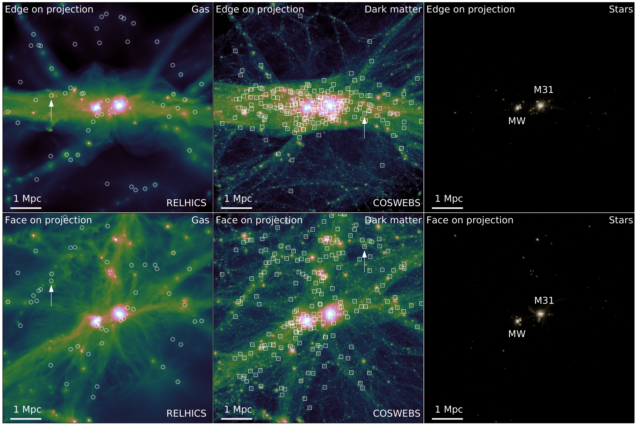
We examine these issues here using the cosmological hydrodynamical simulations of the APOSTLE/EAGLE projects. We focus, in particular, on the gas content of “dark” minihalos. Given their lack of stars, and therefore of any energetic “feedback”, two main mechanisms play a role in setting the gaseous content of minihalos: (i) cosmic reionization, which should evaporate much, but not all, of the baryons from such shallow potential wells, and (ii) ram pressure stripping by the cosmic web, which may unbind the gaseous content from minihalos that travel through dense filaments or “pancakes” of gas. Benítez-Llambay et al. (2013) show that the latter effect may reduce substantially the baryonic content of low-mass halos, especially in high-density regions such as groups of galaxies.
This paper is organized as follows. We begin in Section 2 with a brief summary of the APOSTLE/EAGLE suite of simulations, followed in Section 3 by a discussion of our main results. We analyse the baryon content of dark minihalos in Sec. 3.1. We identify two populations of dark minihalos in Sec. 3.2; one where the properties of the gas component are mainly set by the ionizing background, and another where the gas has been nearly completely removed by cosmic web stripping. We discuss the properties of the former in Sec. 4, where we also present a simple model that reproduces their main structural properties. We use this model to make predictions for their H i content, column density profiles, and 21 cm line widths, and compare them with the properties of UCHVCs in Sec. 4.5. We conclude with a brief summary of our main conclusions in Sec. 5, and provide an appendix with an analytic model for the gas density and temperature profiles in minihalos.

2 Numerical Simulations
2.1 The APOSTLE project
We use a suite of cosmological hydrodynamical simulations from the APOSTLE33 3 APOSTLE stands for “A Project Of Simulating The Local Environment” project (Fattahi et al., 2016; Sawala et al., 2016). These are zoom-in simulations that follow the formation of various Local Group-like cosmological environments. Twelve different realizations are followed at three different resolutions (L1, L2, and L3, in order of decreasing resolution). All volumes are selected from the DOVE N-body simulation (Jenkins, 2013) using the criteria described in Fattahi et al. (2016). DOVE adopted a cosmological model with parameters consistent with WMAP7 measurements (Komatsu et al., 2011), listed in Table 1.
| ID | ||||
|---|---|---|---|---|
Each simulated volume contains a relatively isolated pair of halos of combined virial mass in the range -; the two halos (meant to represent the Milky Way and M31) have separations -, approach with a relative radial velocity - km s-1, and have tangential velocities that do not exceed km s-1 (Fattahi et al., 2016, see ).
Different resolution levels are chosen so that each level improves on the previous by a factor of in particle mass, and a factor of in gravitational force resolution. The highest-resolution level (L1) has a baryon particle mass of (dark matter particles are times heavier), and a Plummer-equivalent gravitational softening of pc. At the time of writing, all twelve volumes have been completed at L3 and L2 resolution but only three volumes (V01, V04, and V11) have also been completed at L1 resolution. We focus on those three volumes in the rest of this paper, although we use results from lower resolution runs to assess the sensitivity of our results to numerical resolution.

APOSTLE simulations were run with the same modified version of the P-Gadget3 code, last described by Springel (2005), which was used to run the simulations of the EAGLE project (Schaye et al., 2015; Crain et al., 2015)The EAGLE code includes a set of subgrid prescriptions to account for the effects of radiative cooling, photoheating, star formation, energy feedback from star formation, and AGN feedback, among others. The adjustable numerical parameters of the subgrid modules were chosen to provide an approximate match to the galaxy stellar mass function and galaxy sizes over cosmological volumes, and correspond to that of the EAGLE ’Reference’ runs. As discussed by Sawala et al. (2016) the three APOSTLE resolutions yield very similar galaxy stellar mass functions (over the range resolved with more than 50 star particles), indicating good numerical convergence in the dwarf galaxy regime probed by APOSTLE. In addition, the APOSTLE galaxy mass-halo mass relation matches rather well the abundance-matching constraints for galaxies in the range (see Fig. 1). We conclude that, at least in the low-mass regime, our results are weakly sensitive to numerical resolution, and we therefore attempt no further parameter recalibration.
2.2 Reionization and the UV background
Cooling and photoheating processes in the EAGLE code are implemented following the procedures outlined in Wiersma et al. (2009). In brief, the thermodynamic state of the gas is modelled using CLOUDY (Ferland et al., 1998), assuming ionization equilibrium with the cosmic microwave background (CMB) and a spatially uniform evolving UV/X-ray background radiation field as calculated by Haardt & Madau (2001) (HM01 thereafter) in the optically thin regime. The simulation neglects self-shielding which could have an impact on regions with , and temperatures below (Schaye, 2001; Rahmati et al., 2013, see, e.g,)44 4 Our study focuses on systems with gas densities and temperatures . Self-shielding could in principle change the properties of some of these systems since the temperature would be slightly reduced, thus increasing the H i mass predicted in Sec. 4.4.. Reionization of the Universe is modelled by switching on the HM01 background radiation field at redshift . The photoheating and photoionizing rates are kept fixed in the redshift range . For redshift , the UV background is allowed to evolve, and reaches a maximum at redshift . In addition, an extra heating of 2eV per proton mass is injected to the gas particles at , which accounts for a boost in the photoheating rates during reionization relative to the optically thin rates assumed here, ensuring that the photoionized gas is rapidly heated to a temperature of . This is done instantaneously for H , but for He ii the extra heat is distributed in redshift with a Gaussian of width , centred at .
For redshift , the net cooling55 5 We refer to the net cooling of the gas as the difference between the radiative heating and cooling processes. of the gas is computed by exposing it to the CMB and the photodissociating background obtained by cutting the HM01 spectrum at 1 Ryd. Note that the presence of photodissociating radiation and the finite resolution of our simulations imply that we cannot model the formation of Pop III stars via cooling in minihalos, which could play a role for isolated halos of mass .
2.3 Halo finding
Halos are identified in the simulations using the group finder SUBFIND (Springel et al., 2001; Dolag et al., 2009), which identifies self-bound substructures within a catalogue of friends-of-friends (FoF) halos built with a linking length of 0.2 times the mean interparticle separation. SUBFIND provides a list of self-bound subhalos within each FoF halo, organized as a “central” halo and its respective “satellites”.
Most of our analysis is based on central halos identified at redshift within a spherical volume of radius centred at the barycentre of each simulated “Local Group”. We keep for analysis all central halos with (i.e., with typically more than dark matter particles). These limits in volume and mass ensure that all selected halos are far enough from the boundaries of the high-resolution zoom-in region and that we are able to resolve them confidently.
3 Results
3.1 Baryonic content of APOSTLE halos

We begin by analysing the baryonic content within the virial boundaries of the simulated halos. This is presented in the top panel of Figure 1, where we show the relation between virial mass and the mass of various baryonic components for the three “high-resolution” volumes. The oblique dashed line indicates, for reference, the theoretical maximum baryonic mass within the virial radius, , where is the universal baryon fraction.
The blue solid line indicates the median stellar mass "bound" to the central galaxies. Note that we only consider “central” galaxies in this figure; i.e., the most massive subhalo of each FoF halo.
The median stellar mass plummets below a virial mass of , mainly because not all those low-mass halos harbour luminous galaxies. This may be seen from the thick black dashed line in the bottom panel of Fig. 1, which shows the fraction of central galaxies that do not have stars. All halos above have luminous galaxies, but the fraction dips to at . Below essentially all halos are ‘‘dark’’66 6 Strictly speaking, these halos have galaxies less massive than a few in stars, the mass of one baryon particle at this resolution level..
The median total baryon mass bound to luminous halos, measured within , is shown by the green curve in Fig. 1, with a shading that indicates dispersion. The total gas mass within bound77 7 We note that SUBFIND can at times underestimate these masses, especially in regions where the mean ambient gas density is comparable to the density in the outer regions of the minihalo or when a minihalo is embedded in hotter gas; the masses shown here have been carefully recomputed to take those issues into account. to “dark” (i.e., star free) halos is shown with open circles. Two populations are clearly apparent: one where the bound gas mass is so small (, shown in grey) that it can barely be measured (the gas particle mass is at resolution level L1); and another where the gas mass correlates tightly with virial mass (shown in red). We shall hereafter refer to the former as “COSWEBs” (short for cosmic web-stripped halos) and to the latter as “RELHICs” (for Reionization-Limited H i Clouds).
Before discussing the origin of these two populations, we show in the bottom panel of Fig. 1 their relative fractions as a function of mass, as well as the dependence on numerical resolution. The thick solid red curve indicates the fraction of RELHICs in the highest-resolution (L1 level) runs: RELHICs inhabit halos spanning a small range in virial mass, , making up about half of all systems at the mid point of that range. Lower-resolution simulations (L2 runs, shown with a dot-dashed line), as well as simulations of a larger volume88 8 EAGLE run Recal-L025N0752. at L2 resolution yield RELHIC fractions similar to that of L1 runs at the high-mass end of the range, but underestimate their abundance at the low-mass end, below a virial mass of . The drop in RELHIC fractions below that mass is mainly a result of limited numerical resolution. As we discuss below, the main difference between RELHICs and COSWEBs is environmental, so we would expect the ratio of the two to approach a constant at low virial masses. Interestingly, although not shown here, RELHICs in all of these runs track the same gas mass-virial mass trend shown in the upper panel of Fig. 1, regardless of resolution.

3.2 COSWEBs and RELHICs
The spatial distribution of the two populations (RELHICs and COSWEBs) are clearly different, as shown in Fig. 2, hinting at an environmental origin of their distinction. This figure shows two orthogonal projections of one APOSTLE volume run at the highest-resolution (V01-L1): the two main LG galaxies are clearly visible near the centre, surrounded by a two-dimensional “sheet” of gas that extends out to several Mpc from the LG barycentre. COSWEBs, shown as open squares in the middle panels, cluster around the main galaxies and inhabit the mid plane of the sheet, whereas RELHICs (open circles in the left panels) populate underdense regions in the periphery of the LG volume.
The evolution of a typical COSWEB is shown in Fig. 3. The top left panel shows the evolution of the various mass components, measured within the virial radius of the most massive progenitor. As expected, the dark mass grows monotonically, with occasional jumps corresponding to merger events. The gas mass largely follows suit, except at late times, when it drops dramatically, in this example at . The drop is more clearly seen in the bottom left panel, which tracks , the baryon fraction of the halo expressed in units of the universal baryon fraction.
The four panels on the right of Fig. 3 show snapshots of the gas component at different stages of the evolution, at times marked by the solid circles in the left panels. The top two right panels show the COSWEB just before and after reionization, when the gas is suddenly heated to K, a temperature that exceeds the virial temperature of the halo at that time (see the bottom green curve, which tracks K). The gas is therefore too hot to remain bound, and evaporates from the potential well of the halo. By , the halo has only been able to retain about th of its baryons. Just after , however, the COSWEB travels through an overdense region of the cosmic web, which ram-pressure strips the remainder of the gas, reducing its bound gas content to a negligible amount. The COSWEB is unable to re-accrete gas by redshift , mainly because it is now moving relatively fast within the much hotter LG environment. COSWEBs are thus star/gas-free minihalos whose gaseous content has been removed by the cosmic web (see Benítez-Llambay et al., 2013, for a more extensive discussion of cosmic web stripping).
By contrast, RELHICs are minihalos that have avoided dense regions of the cosmic web, and have therefore been able to retain more baryons. The evolution of a typical RELHIC is shown in Fig. 4. Comparing this to that of the COSWEB in Fig. 3, we see that the main difference is that the RELHIC baryon fraction remains more or less constant after the initial drop caused by reionization. At this particular RELHIC has been able to retain about th of the universal baryon fraction. What sets the final baryon content of RELHICs and, in particular, what is the origin of the strong correlation between bound gas mass and virial mass shown in Fig. 1? We address these questions next.
4 RELHICs
4.1 Gas densities and temperatures
We start by considering the thermodynamic state of the gas in RELHICs. This is shown in Fig. 5, where we plot the density and temperature of all gas particles bound to the 249 RELHICs identified in all three simulated volumes. We have excluded 9 RELHICs (i.e., per volume) with masses , whose central gas densities reach values , and thus their central thermodynamic properties are expected to be governed by the effective equation of state imposed in the EAGLE code on the unresolved multiphase interstellar/star forming medium.
The gas in the remaining RELHICs spans nearly seven decades in density, from the mean baryon density of the Universe () to densities 100 times below the threshold chosen for star formation in EAGLE (cm-3 for a gas with primordial composition)99 9 We discuss the impact of the particular choice of the star formation density threshold on our results in Appendix B.. Gas temperatures are a non-monotonic function of density, first climbing to a maximum of at , and then dropping gradually at higher densities, approaching .
The gas is, on average, hotter than the virial temperature of a typical RELHIC ( for a virial mass of ), implying that the gas temperature is largely set by the ionizing background, and not by the gravitational collapse of the halo. This is further demonstrated by the green dashed curve, which indicates where the photoionizing heating time-scale equals the age of the Universe, . Temperatures of low density gas in RELHICs are clearly set by the ionizing background.
At densities cm-3 radiative cooling induced by collisional effects becomes more important and the gas settles at the “equilibrium” temperatures where radiative cooling effects balance photoheating from the ionizing background, shown by the thick purple line in Fig. 5 (Haehnelt et al., 1996; Theuns et al., 1998, see e.g.,). As is clear from this figure, these two regimes describe very well the temperature-density relation of gas in RELHICs (shown by the red dashed curve).
4.2 Gas masses
The - relation followed by gas particles in RELHICs effectively defines a pressure-density relation, , that enables us to estimate the gas mass bound to a halo of given virial mass. This may be done by assuming that the gas is in hydrostatic equilibrium within the potential of the dark halo and solving:
| (1) |
to give a density profile that may be integrated to compute the total gas mass within , once a boundary condition (e.g., an external pressure) is chosen.
The simplest choice is to assume that far from the virial boundary the gas reaches the mean baryon density of the Universe, at the appropriate temperature set by the ionizing background: this specifies the external pressure that closes the set of equations, enabling a simple estimate of RELHIC gas masses.
We present details of the calculation in Appendix A and show the main result by the thick purple line in Fig. 1. Despite its simplicity, the model predicts accurately the gas mass of RELHICs for halos not exceeding virial masses of order . At higher masses gravitational heating becomes important and, in addition, the central densities become high enough for self-shielding and cooling processes to become important; in those halos the gas would not be able to stay in hydrostatic equilibrium, but will collapse into a rotationally supported disk where it may form stars. Indeed, very few, if any, halos above remain “dark”, as shown in the bottom panel of Fig. 1.
4.3 Gas and temperature profiles
We may test further the simple hydrostatic model described in Appendix A by using it to predict the density and temperature profiles of the gas component of RELHICs and comparing them with the simulation results. Figure 6 shows an example for a relatively massive RELHIC; and .
We first measure the acceleration profile of the halo, assuming spherical symmetry: , where is the total enclosed mass within radius . Baryons contribute so little mass that this is effectively equivalent to the dark matter acceleration profile. We show in the top left panel of Fig. 6 by the solid black line. The red dashed curve is a fit to this acceleration profile, namely, a Navarro-Frenk-White (Navarro et al., 1996; Navarro et al., 1997, hereafter NFW) profile with concentration parameter .
We then integrate Eq. 1 numerically, using a fit to the temperature-density relation (see the red dashed curve in the inset of the bottom right panel of Fig. 6), and normalizing the profile at the radius that contains half of all gas particles1010 10 This normalization procedure improves fits to individual halos, but its results are not very different from those obtained assuming the simple boundary condition that the gas profile should converge to the mean density of the Universe at large radii.. The result for the density profile may be seen in the top right panel of Fig. 6. Clearly the predicted profile is in excellent agreement with the simulation (dots correspond to individual gas particles in the simulation).
The model temperature profile is shown in the bottom left panel of the same figure and is also in excellent agreement with the results from the simulation. We have verified that the model works equally well for other RELHICs of different masses. We have also verified that the overall properties of RELHICs are relatively insensitive to our choice of UV background. This may be seen in the inset of Figure 6, where the dot-dashed curve shows the equilibrium temperature-density relation obtained if the intensity of the UV background is increased to match the HM01 spectrum. Using that relation leads to changes in the gas mass predicted for RELHICs smaller than .
This analysis demonstrates that the gas in RELHICs is in hydrostatic equilibrium with the halo potential and that a simple model allows us to predict the mass, structural parameters, and radial profiles of the gas component of these “dark” minihalos accurately. In particular, we may use the same model to predict the neutral hydrogen content of RELHICs, an issue to which we turn next.

4.4 HI masses and radial profiles
The blue solid lines in Fig. 6 show the density profiles of neutral hydrogen, derived using the fitting formula given in appendix A1 of Rahmati et al. (2013). This model uses a simple but accurate fit to the photoionization rates, obtained from radiative transfer simulations, where the scaling of the characteristic self-shielding density is taken from the analytic model of Schaye (2001), and computes neutral fractions as a function of density and temperature assuming ionization equilibrium. In the inner regions of the example RELHIC shown in Fig. 6 the gas is dense and cold enough to be neutral; the neutral fraction drops rapidly from the center outwards. The H i column density profile is shown in the bottom right panel of Fig. 6: the profile is quite steep, in part due to the onset of self-shielding in the model, and it drops from a well-defined central value of cm-2 to cm-2 at kpc from the centre1111 11 We compute the column density profiles by integrating the density profile along the line-of-sight within a sphere of radius ..
We show the gas density and H i column density profiles in Fig. 7, as a function of halo virial mass or, equivalently, as a function of the total gas mass. RELHICs have density profiles that vary in shape as the halo mass decreases, and central densities that correlate strongly with mass. Although the most massive RELHICs may reach central H i column densities of cm-2 these drop steeply with decreasing mass, dipping below cm-2 for halos below . This suggests that only the most massive RELHICs might be detectable in 21 cm surveys such as ALFALFA (Haynes et al., 2011, e.g.,), which only reaches column densities exceeding cm-2.
We provide further structural properties of the H i component of RELHICs in Fig. 8, where we show the total H i mass within as a function of central H i column density and as a function of the total gas mass (left panels). The dashed lines show the results of the model described in Appendix A ( Fig. 7), which agree very well with the simulation results. Clearly, neutral hydrogen makes up a very small fraction of the gaseous content of minihalos, confirming the expectations of the analytic models of Sternberg et al. (2002): minihalos are essentially spheres of ionized gas in hydrostatic equilibrium and they have a small core of neutral hydrogen.
The bottom right-hand panel of Fig. 8 shows several characteristic radii, where the RELHIC H i column density drops from its central value to , ,…, cm-2, respectively (top to bottom). The dashed lines indicate the results of the model profiles shown in Fig. 7, whereas the open circles correspond to simulated RELHICs, grouped so that each is plotted at the radius where the column density drops by about one decade (or less) from the center. For example, the radii shown for RELHICs with central column densities between and cm-2 is that where the column density drops to cm-2, and so on. Note that, defined this way, most RELHICs within reach of current H i surveys (i.e., ; cm-2) are expected to be compact, sub-kpc systems (Sternberg et al., 2002).
RELHICs are near hydrostatic equilibrium, so the random bulk motions of the gas are quite small compared with the characteristic velocity dispersion of the halos they inhabit. This may be seen in the top right panel of Fig. 8, where we show, as a function of the total gas mass within , the velocity dispersion of RELHIC gas particles, compared with the characteristic rms velocities of dark matter particles, . Typical bulk motions in RELHICs are below km/s in essentially all cases, well below , implying that the broadening of the 21 cm line should be mostly thermal.
Finally, we examine the morphologies of RELHICs in Fig. 9, which shows H i column density maps for relatively massive RELHICs (see masses in figure legends). Drawing attention to the cm-2 contour (black thick inner line), which corresponds to the sensitivity limit of surveys such as ALFALFA, we see that RELHICs would appear essentially round in such surveys. This is a direct consequence of the fact that the gas is in hydrostatic equilibrium in the dark halo potential. Indeed, although CDM halos are intrinsically triaxial, the axis ratios of the potential are much less aspherical than those of the mass distribution (Hayashi et al., 2007, see, e.g.,).
4.5 UCHVCs as Local Group RELHICs
We explore now the possibility that RELHICs might have been detected already in existing H i surveys. Given their sizes and low H i masses, we compare RELHICs with the population of Ultra Compact High Velocity Clouds (UCHVCs) first discussed by Giovanelli et al. (2010) in the context of the ALFALFA survey. These are identified as high signal-to-noise H i sources with sizes less than , and velocities well outside the range expected for Galactic rotation. Note that corresponds to kpc at a distance of kpc, so these sources might include sub-kpc RELHICs in the Local Group.
We begin by noting that, as shown in Fig. 2, RELHICs shun the region close to the Local Group barycentre and mainly populate the underdense regions of its outskirts. Indeed, we find no RELHIC within kpc of any of the two main LG galaxies in any of the three "high-resolution" volumes we have analysed. This has two important consequences; one is that, coupled with the low H i masses expected of RELHICs, their H i fluxes will be quite low, and another is that few RELHICs will have negative Galactocentric radial velocities, as most will still be expanding away outside the LG turnaround radius.
We show this in Fig. 10, where we show, as a function of the H i flux1212 12 We compute H i fluxes using the total H i mass within the virial radius of a RELHIC, , and its distance to the LG primary galaxies expressed in Mpc, : , with given in units of Jy km/s. Note that as we consider the two main galaxies of each simulated LG, every RELHIC is shown twice in Fig. 10., , in units of , the H i size of the RELHIC, defined as the mean radius , where and are the semiaxes of the best fitting ellipse to its cm-2 isodensity contour (top panel), Galactocentric radial velocity, (second from top), the FWHM line broadening parameter1313 13 is computed by adding in quadrature the broadening due to the gas temperature and its bulk velocity dispersion. The former dominates, and is given by K, with given in km/s., (third from top), and the axis ratio of the limiting H i column density isocontour, (bottom panel).
Fig. 10 compares simulated RELHICs (open red circles) and luminous simulated dwarfs (; magenta circles), with the UCHVCs catalogued by Adams et al. (2013) from ALFALFA data (see black crosses). The stellar mass limit roughly corresponds to that of Leo P, which was discovered after follow-up imaging of an UCHVC (Giovanelli et al., 2013). Note that all APOSTLE RELHICs are just below the flux limit of the ALFALFA search, which is of Jy km/s (shown by the vertical dashed line). UCHVCs are also much more numerous and heterogeneous as a population than expected for RELHICs, which are rather small; fairly round (); have a narrow dispersion of linewidths about km/s; and are almost exclusively moving away from the Galaxy. UCHVCs are, however, comparable to simulated dwarfs, which reach higher fluxes, exhibit a wider range of morphologies, and are bigger than RELHICs. We do not analyse the distribution of for our simulated dwarfs as their temperature is set by a an effective equation of state imposed to model the ISM, which is set to . Because of this, the HI fluxes estimated for dwarfs must be regarded as lower limits.
We conclude that the Adams et al. (2013) UCHVC catalogue does not contain the star-free “dark” minihalos we associate with RELHICs, and that the properties of some UCHVCs might be consistent with very faint dwarf galaxies that have so far escaped detection in optical surveys. Indeed, as discussed in Sec. 1, some UCHVCs have already been identified as low surface brightness galaxies, some in the Local Volume (Sand et al., 2015) and some as far away as the Virgo Cluster (Bellazzini et al., 2015b).
5 Summary and Conclusions
We have used the APOSTLE suite of cosmological hydrodynamical simulations of the Local Group to examine the gas content of CDM minihalos. We focussed our analysis on systems that are free of stars in our highest-resolution runs, since in such systems the bound gas content at should only depend on the effects of the UV ionizing background and on the ram pressure stripping that affects minihalos as they travel through the cosmic web.
“Dark” minihalos (or, more precisely, systems with stellar mass , the mass resolution limit of our simulations) split into two well-defined groupings: one where the mass of bound gas is set by the ionizing background and correlates tightly with the minihalo virial mass (RELHICs, for REionization Limited H i Clouds), and another where there is little or no bound gas left within the halo after stripping by the cosmic web (COSWEBs, for COSmic WEb Stripped systems). The differentiation is thus mainly environmental; gas-free COSWEBs populate the high-density regions near the luminous galaxies of the Local Group, where gas densities are high and cosmic web stripping is important, whereas the relatively gas-rich RELHICs inhabit the underdense outskirts. Few RELHICs are found within kpc of either the Milky Way or the M31 analogues in the simulations.
In terms of halo virial mass, the transition between luminous galaxies and dark systems like RELHICs and COSWEBs happens relatively quickly. Dark minihalos have masses that do not exceed ; their fraction increase rapidly with decreasing mass, and they make up essentially all halos below . RELHICs make up most of the more massive dark minihalos; their abundance peaks at roughly for . The RELHIC bound gas mass fraction decreases with decreasing mass; from of the universal baryon fraction at to (, or ten particles in our highest-resolution runs) in minihalos.
The gas component in RELHICs is in approximate hydrostatic equilibrium with the dark matter potential and in thermal equilibrium with the ionizing UV background. Their thermodynamic properties are therefore well understood, and their gas density and temperature profiles are in excellent agreement with a simple model where UV-heated gas is in thermal and hydrostatic equilibrium within NFW halos. Gas in RELHICs is nearly pristine in composition and nearly fully ionized, with small (sub-kpc) neutral hydrogen cores that span a large range of H i masses and column densities. These cores have negligible Doppler broadening and nearly round morphologies.
The most massive RELHICs have properties comparable to those of some Ultra Compact High Velocity Clouds (UCHVCs) but the bulk of the Local Group RELHIC population should have H i fluxes just below Jy km/s, the limit of the ALFALFA UCHVC detection.
Other differences between RELHICs and UCHVCs are the following: (i) the sheer number of UCHVCs implies that most UCHVCs are not RELHICs (we expect fewer than 10 Local Group RELHICs with Jy km/s over the whole sky); (ii) RELHICs should mostly reside beyond kpc from the Milky Way, leading to low H i fluxes ( Jy km/s), very small angular sizes (), and predominantly positive Galactocentric radial velocities; (iii) RELHICs should be nearly round on the sky ( at cm-2) and (iv) have a very narrow distribution of thermally broadened line widths ( km/s).
The small overlap in properties between UCHVCs and RELHICs suggest that the former are not part of the abundant dark minihalo population expected in the CDM models. UCHVCs are either H i “debris” in the Galactic halo, or else the H i component of more massive halos, most of whom are expected to host a luminous stellar component as well. Further work is underway that aims to clarify the overall abundance of RELHICs in cosmological volumes; their contribution to the low-mass end of the H i mass function; their relation to ultra faint galaxies; and the best strategies to detect them. Although RELHICs seem too faint to be a dominant source of H i detections in extant or planned surveys, they may be easier to detect and study in absorption against the light of luminous background objects at moderate redshifts. RELHICs are a robust prediction of the CDM paradigm so their detection and characterization would offer a unique opportunity to shed light onto the “dark” side of a cold dark matter-dominated universe.
6 Acknowledgements
We acknowledge useful discussions with John Cannon, Luke Leisman, Manolis Papastergis, Antonino Marasco and Tom Osterloo. We also thank the anonymous referee for valuable comments that helped to improve the paper. We have benefited from the following public Python packages: numpy (Van Der Walt et al., 2011), scipy (Jones et al., 2001), matplotlib (Hunter, 2007), Ipython (Pérez & Granger, 2007) and py-sphviewer (Benitez-Llambay, 2015). RCA is a Royal Society University Research Fellow. This work was supported by the Science and Technology Facilities Council (gran number ST/L00075X/1) and the European Research Council (grant numbers GA 267291 "Cosmiway"). It was also partially supported by the Interuniversity Attraction Poles Programme initiated by the Belgian Science Policy Office ([AP P7/08 CHARM]), and by the European Research Council under the European Union’s Seventh Framework Programme (FP7/2007-2013)/ERC grant agreement 278594-GasAround Galaxies and by the Netherlands Organisation for Scientific Research (NWO) through VICI grant 639.043.409. This work used the DiRAC Data Centric system at Durham University,operated by the Institute for Computational Cosmology on behalf of the STFC DiRAC HPC Facility (www.dirac.ac.uk). This equipment was funded by BIS National E-infrastructure capital grant ST/K00042X/1, STFC capital grants ST/H008519/1 and ST/K00087X/1, STFC DiRAC Operations grant ST/K003267/1 and Durham University. DiRAC is part of the National E-Infrastructure.
References
- Adams et al. (2013) Adams E. A. K., Giovanelli R., Haynes M. P., 2013, ApJ, 768, 77
- Behroozi et al. (2013) Behroozi P. S., Wechsler R. H., Conroy C., 2013, ApJ, 770, 57
- Bellazzini et al. (2015a) Bellazzini M., et al., 2015a, A&A, 575, A126
- Bellazzini et al. (2015b) Bellazzini M., et al., 2015b, ApJ, 800, L15
- Benitez-Llambay (2015) Benitez-Llambay A., 2015, py-sphviewer: Py-SPHViewer v1.0.0, doi:10.5281/zenodo.21703, http://dx.doi.org/10.5281/zenodo.21703
- Benítez-Llambay et al. (2013) Benítez-Llambay A., Navarro J. F., Abadi M. G., Gottlöber S., Yepes G., Hoffman Y., Steinmetz M., 2013, ApJ, 763, L41
- Blitz et al. (1999) Blitz L., Spergel D. N., Teuben P. J., Hartmann D., Burton W. B., 1999, ApJ, 514, 818
- Braun & Burton (1999) Braun R., Burton W. B., 1999, A&A, 341, 437
- Bullock et al. (2000) Bullock J. S., Kravtsov A. V., Weinberg D. H., 2000, ApJ, 539, 517
- Carlberg (2009) Carlberg R. G., 2009, ApJ, 705, L223
- Charles et al. (2016) Charles E., et al., 2016, Phys. Rep., 636, 1
- Crain et al. (2015) Crain R. A., et al., 2015, MNRAS, 450, 1937
- Dalal & Kochanek (2002) Dalal N., Kochanek C. S., 2002, ApJ, 572, 25
- Diemand et al. (2007) Diemand J., Kuhlen M., Madau P., 2007, ApJ, 657, 262
- Dolag et al. (2009) Dolag K., Borgani S., Murante G., Springel V., 2009, MNRAS, 399, 497
- Fattahi et al. (2016) Fattahi A., et al., 2016, MNRAS, 457, 844
- Feldmann & Spolyar (2015) Feldmann R., Spolyar D., 2015, MNRAS, 446, 1000
- Ferland et al. (1998) Ferland G. J., Korista K. T., Verner D. A., Ferguson J. W., Kingdon J. B., Verner E. M., 1998, PASP, 110, 761
- Garrison-Kimmel et al. (2014) Garrison-Kimmel S., Boylan-Kolchin M., Bullock J. S., Lee K., 2014, MNRAS, 438, 2578
- Giovanelli & Haynes (2016) Giovanelli R., Haynes M. P., 2016, A&ARv, 24, 1
- Giovanelli et al. (2010) Giovanelli R., Haynes M. P., Kent B. R., Adams E. A. K., 2010, ApJ, 708, L22
- Giovanelli et al. (2013) Giovanelli R., et al., 2013, AJ, 146, 15
- Haardt & Madau (2001) Haardt F., Madau P., 2001, in Neumann D. M., Tran J. T. V., eds, Clusters of Galaxies and the High Redshift Universe Observed in X-rays. (arXiv:astro-ph/0106018)
- Haehnelt et al. (1996) Haehnelt M. G., Rauch M., Steinmetz M., 1996, MNRAS, 283, 1055
- Hayashi et al. (2007) Hayashi E., Navarro J. F., Springel V., 2007, MNRAS, 377, 50
- Haynes et al. (2011) Haynes M. P., et al., 2011, AJ, 142, 170
- Hezaveh et al. (2016) Hezaveh Y. D., et al., 2016, ApJ, 823, 37
- Hunter (2007) Hunter J. D., 2007, Computing In Science & Engineering, 9, 90
- Ibata et al. (2002) Ibata R. A., Lewis G. F., Irwin M. J., Quinn T., 2002, MNRAS, 332, 915
- Ikeuchi (1986) Ikeuchi S., 1986, Ap&SS, 118, 509
- Jenkins (2013) Jenkins A., 2013, MNRAS, 434, 2094
- Johnston et al. (2002) Johnston K. V., Spergel D. N., Haydn C., 2002, ApJ, 570, 656
- Jones et al. (2001) Jones E., Oliphant T., Peterson P., et al., 2001, SciPy: Open source scientific tools for Python, http://www.scipy.org/
- Klypin et al. (1999) Klypin A., Kravtsov A. V., Valenzuela O., Prada F., 1999, ApJ, 522, 82
- Komatsu et al. (2011) Komatsu E., et al., 2011, ApJS, 192, 18
- Mao & Schneider (1998) Mao S., Schneider P., 1998, MNRAS, 295, 587
- Michałowski et al. (2015) Michałowski M. J., et al., 2015, A&A, 582, A78
- Moore et al. (1999) Moore B., Ghigna S., Governato F., Lake G., Quinn T., Stadel J., Tozzi P., 1999, ApJ, 524, L19
- Moster et al. (2013) Moster B. P., Naab T., White S. D. M., 2013, MNRAS, 428, 3121
- Navarro et al. (1996) Navarro J. F., Frenk C. S., White S. D. M., 1996, ApJ, 462, 563
- Navarro et al. (1997) Navarro J. F., Frenk C. S., White S. D. M., 1997, ApJ, 490, 493
- Pérez & Granger (2007) Pérez F., Granger B. E., 2007, Computing in Science and Engineering, 9, 21
- Rahmati et al. (2013) Rahmati A., Pawlik A. H., Raicevic M., Schaye J., 2013, MNRAS, 430, 2427
- Rauch (1998) Rauch M., 1998, ARA&A, 36, 267
- Rees (1986) Rees M. J., 1986, MNRAS, 218, 25P
- Sand et al. (2015) Sand D. J., et al., 2015, ApJ, 806, 95
- Saul et al. (2012) Saul D. R., et al., 2012, ApJ, 758, 44
- Sawala et al. (2016) Sawala T., et al., 2016, MNRAS, 457, 1931
- Schaye (2001) Schaye J., 2001, ApJ, 562, L95
- Schaye (2004) Schaye J., 2004, ApJ, 609, 667
- Schaye et al. (2015) Schaye J., et al., 2015, MNRAS, 446, 521
- Springel (2005) Springel V., 2005, MNRAS, 364, 1105
- Springel et al. (2001) Springel V., White S. D. M., Tormen G., Kauffmann G., 2001, MNRAS, 328, 726
- Springel et al. (2008) Springel V., et al., 2008, Nature, 456, 73
- Sternberg et al. (2002) Sternberg A., McKee C. F., Wolfire M. G., 2002, ApJS, 143, 419
- Theuns et al. (1998) Theuns T., Leonard A., Efstathiou G., Pearce F. R., Thomas P. A., 1998, MNRAS, 301, 478
- Van Der Walt et al. (2011) Van Der Walt S., Colbert S. C., Varoquaux G., 2011, Computing in Science & Engineering, 13, 22
- Vegetti et al. (2010) Vegetti S., Koopmans L. V. E., Bolton A., Treu T., Gavazzi R., 2010, MNRAS, 408, 1969
- White & Rees (1978) White S. D. M., Rees M. J., 1978, MNRAS, 183, 341
- Wiersma et al. (2009) Wiersma R. P. C., Schaye J., Smith B. D., 2009, MNRAS, 393, 99
Appendix A Analytic model for RELHICs
We showed in Figure 5 that the relation followed by gas particles in RELHICs effectively defines an equation of state, . Thus, heating and cooling processes couple the temperature of the gas to its density. We use this fact to derive a simple model that accounts for all the thermodynamic properties of RELIHCs. Our model relies on two main assumptions: 1) spherical symmetry and 2) hydrostatic equilibrium between the gas content of the halos and the gravitational potential, largely due to the dark matter distribution.
We start by assuming a gaseous halo in hydrostatic equilibrium with its spherically symmetric potential, so that the pressure gradient is balanced by the halo gravitational acceleration:
| (2) |
where is the circular velocity of the halo at the virial radius and is the (normalized) enclosed mass within a sphere of radius . For an ideal gas, the relation between pressure, density and temperature is given by:
| (3) |
where is the Boltzmann constant, is the gas mean molecular weight, is the proton mass and is the adiabatic index or ratio of specific heats. Throughout this paper we use and , although allowing to vary might lead to an improvement of the model.
Equation 2 can be solved if we know the pressure at a particular radius, or equivalently, the density and the temperature at that radius. However, for our particular purposes the gas temperature is defined by its density, and thus the pressure is set by the gas density only, so that Eq. 2 can be rewritten as:
| (4) |
where we have introduced the virial temperature
| (5) |
Assuming that the halo potential is largely due to the underlying dark matter distribution, we can model it with a NFW mass profile, so that the acceleration profile is:
| (6) |
where is the concentration parameter.
We now study the asymptotic behaviour of the model. At small radii, (), the gas density converges as . In fact, the integral of the acceleration profile is:
| (7) |
For larger distances, , the acceleration profile vanishes, thus implying that the density eventually reaches a constant value. Moreover, for a sufficiently isolated halo, the density will reach the mean gas density of the Universe at larger radii. This simple and theoretically motivated boundary condition is in fact the only free parameter of the model, and enables us to predict the gas mass within , as a function of , as shown by the purple solid line in Figure 1, and it is enough to derive all other properties shown in Figures 7, 8, 9 and 10.
| -8.0 | 2.91 | -3.8 | 4.38 |
| -7.8 | 3.02 | -3.6 | 4.32 |
| -7.6 | 3.13 | -3.4 | 4.28 |
| -7.4 | 3.24 | -3.2 | 4.24 |
| -7.2 | 3.36 | -3.0 | 4.20 |
| -7.0 | 3.47 | -2.8 | 4.17 |
| -6.8 | 3.59 | -2.6 | 4.14 |
| -6.6 | 3.70 | -2.4 | 4.12 |
| -6.4 | 3.81 | -2.2 | 4.10 |
| -6.2 | 3.93 | -2.0 | 4.08 |
| -6.0 | 4.04 | -1.8 | 4.06 |
| -5.8 | 4.15 | -1.6 | 4.04 |
| -5.6 | 4.25 | -1.4 | 4.03 |
| -5.4 | 4.35 | -1.2 | 4.01 |
| -5.2 | 4.44 | -1.0 | 4.00 |
| -5.0 | 4.51 | -0.8 | 3.99 |
| -4.8 | 4.54 | -0.6 | 3.97 |
| -4.6 | 4.54 | -0.4 | 3.96 |
| -4.4 | 4.51 | -0.2 | 3.95 |
| -4.2 | 4.49 | 0.0 | 3.94 |
| -4.0 | 4.43 |
In practice, we solve Eq. 4 numerically, imposing the relation between temperature and density shown by the red-dashed line in Figure 5 (given in Table 2 for completeness), and fitting a NFW acceleration profile to the mass distribution of the simulated halos. In brief, we solve:
| (8) | |||||
| (9) |
and the spatial dependence of density is obtained by inverting F:
| (10) |
For low-density gas (), is well approximated by a power law, and an analytical solution can be given. In fact, assuming
| (11) |
where , and , it is straightforward to integrate Eq. 4 to obtain the gas density profile:
| (12) |
Appendix B Star formation density threshold
Star formation typically occurs when gas is able to develop a cold phase. We note, however, that our simulations lack the physics needed to simulate the transition between the warm and cold phase self-consistently, so that gas particles are eligible to form stars once they reach densities above a given threshold, , at a temperature of . In APOSTLE we use a density threshold that depends on metallicity, as proposed by Schaye (2004):
| (13) |
which takes into account that the transition between warm, neutral phase to a cold, molecular one occurs at lower densities in more metal-rich gas. Eq. 13 is strictly valid for , and thus the maximum threshold, , valid for the extremely low metallicity RELHICs, is somehow arbitrary. We note, however, that in low-metallicity systems, gas may become cold and form stars without developing a molecular phase (Michałowski et al., 2015, see, e.g.,), a mechanism that cannot be captured in APOSTLE. We can study, however, the impact of choosing a different density threshold for star formation in low-metallicity systems. We quantify this in Figure 11, where the cumulative number of RELHICs as a function of their central density is shown. By construction, none of the RELHICs reach central densities above . There are with densities greater than , which were already excluded from analysis (see Sec. 4.1), and with densities above . We conclude that reducing the threshold density for star formation by a factor of respect to the current value would lead to a removal of RELHICs included in our current analysis.