Structure of charmed baryons studied by pionic decays
Abstract
We investigate the decays of the charmed baryons aiming at the systematic understanding of hadron internal structures based on the quark model by paying attention to heavy quark symmetry. We evaluate the decay widths from the one pion emission for the known excited states, , , , and , as well as for the ground states and . The decay properties of the lower excited charmed baryons are well explained, and several important predictions for higher excited baryons are given. We find that the axial-vector type coupling of the pion to the light quarks is essential, which is expected from chiral symmetry, to reproduce the decay widths especially of the low lying baryons. We emphasize the importance of the branching ratios of for the study of the nature of higher excited baryons.
pacs
14.20.Lq, 13.30.Eg, 12.39.JhI Introduction
Understanding of the internal structure of hadrons is an important subject in hadron physics. One of the most important problems is to identify the effective degrees of freedom which should play essential roles at low energies, because the bare quarks do not appear at such a scale due to the color confinement of QCD. To identify the effective degrees of freedom should serve not only for the understanding of the QCD vacuum properties, but also be useful to explain and predict experimental data with simple physical terms. In this respect, what we are aiming at is to establish the economized effective degrees of freedom for various phenomena of the strong interaction physics [1, *Weinberg:1965zz, 3].
The charmed baryons, containing a single heavy charm quark, is a good place to study the hadron structure. One of the important features is the spin symmetry of the heavy quark. QCD predicts that the spin-dependent interaction of the heavy quark is suppressed by and thus in the infinite limit, the heavy quark spin is decoupled from the dynamics of the light quarks. The dynamical decoupling of the light quark spin and the heavy quark spin is the heavy quark symmetry (HQS) [4].
In the heavy quark limit, the light quark component is called the brown muck as the colorful object conserving its total spin [5]. In terms of QCD, the brown muck contains not only light quarks but also light antiquarks as well as gluons. For the spin of the brown muck , the heavy hadrons are classified to one state with the total spin for and two degenerate states with the total spin for . The former is called the HQS singlet, and the latter is called the HQS doublet. The classification based on the HQS is useful for the investigation of the heavy hadrons, because the brown muck spin serves as an additional conserved quantum number reflecting the internal structure of the heavy hadrons. The HQS appears in many properties of heavy hadrons, such as the mass spectrum and the decay branching ratios11 1 The heavy quark symmetry can be applied also to exotic heavy hadrons such as hadronic molecules [6, 7, 8, 9, 10, 11, 12, 13, 14, 15, 16] as well as to the heavy hadrons in nuclear medium [16, 17, 18, 19, 20, 21, 22]. See Ref. [23] as a review for the latter..
There is another interesting feature of the charmed baryons. In the quark model description, we have two different orbital motions in the low energy excitations. One is the relative motion between two light quarks, so-called -mode. The other is the one between the center-of-mass of the two light quarks and the charm quark, so-called -mode. Owing to the mass difference of the light and heavy quarks, the excitation energies of the - and -modes are kinematically well separated, and the internal excitations are dominated exclusively by either -mode or -mode with only small mixing [24]. This contrasts with light quark baryons where the two modes generally mix largely, and thus is the reason that we can study the two basic modes exclusively in the heavy baryons.
In general, internal structures of hadron are reflected not only in mass spectrum but also in various transition properties such as productions and decays. Among them, two-body decay processes through the one-pion emission are particularly interesting due to the following reasons: (i) The pion couples only to the light quarks, and the charm quark behaves simply as a spectator. The dynamics of the pion is governed by chiral symmetry in a unique manner. Therefore, the transitions accompanying pion emission should bring important information about the dynamics of the two light quarks in a heavy baryon. This is also helpful to understand diquark properties in a heavy baryon. (ii) Some low-lying states of excited charmed baryons have significantly smaller excitation energies than light baryon excitations, and the emitted pion carries only a small momentum. Therefore, the pion emission from the excited charmed baryons is a good place to study the quark-pion interaction, which should be well determined by the low energy chiral dynamics. This can be checked by comparing the theoretical results with the observed decays of the low-lying charmed baryons.

In this paper we consider the pion emission decays from the orbitaly excited charmed baryons 22 2 In this article, we express the ground and excited charmed baryons as and . , , , , into and , and those from orbital ground state charmed baryons and into . The decay paths are summarized in Fig. 1. To estimate the decay widths numerically, we employ a non-relativistic constituent quark model with a harmonic oscillator potential as the quark confinement force. The model is rather simple but we expect that essential and universal features can be extracted.
There are previous works investigating strong decays of charmed baryons [4, 26, 27, 28, 29, 30, 31, 32, 19]. In Ref. [31], based on heavy hadron chiral perturbation theory the importance of heavy quark symmetry are discussed in the heavy quark limit. In Ref. [19], including the correction terms from the next-to-leading order , relationships between decay widths in several decay channels were obtained. In Ref. [32], non-relativistic quark model calculations were performed and decays of various quark model states were investigated. In the present study, we will also employ the non-relativistic quark model. It is worthwhile to emphasize the difference between the works in Ref. [32] and ours. In Ref. [32], the baryon wave functions are constructed in the so-called coupling scheme, while we do in the coupling scheme where the brown muck total is first formed. In doing so, we will derive various relations and selection rules in relation to HQS.
In our study, we will shed light upon the following issues. Firstly, we check the validity of the present framework by calculating the decay widths of the two baryons, and , which are the orbital ground state of charmed baryons. These baryons decay into as the only possible channel in strong decay. Because both the initial and final charmed baryon states are in the orbital ground states in the quark model, those charmed baryons are good objects for confirmation of the validity of our formalism for the one-pion emission. We will see that our results are in reasonably good agreement with the experimental values.
Secondly, we investigate the decay properties of the and as the lowest-lying orbital excitations in -wave. They are interesting because they have the subcomponent, the spin-0 diquark system, which is moving in the -wave orbital of the -mode [33, 28, 34]. They have been observed in collisions and collisions [35, 36, 37] as well as in photoproductions [38]. An interesting feature of them is that the baryon has a considerably large decay width into channel although its phase space is very small. In contrast, has a very small width although there is sufficiently large phase space in its decay channel . We show that the quark model description with the -mode can explain these decay properties very well for these low-lying states. We find that, to achieve the good agreements, the interaction Lagrangian of the derivative coupling (axial-vector coupling) is needed to reproduce the experimental decay width. This strongly implies that the non-linear chiral dynamics works for the pion and constituent quarks. We will present that especially decay properties of are much affected by the isospin breaking effect near the thresholds.
Thirdly, we study higher excited charmed baryons, , and . Because their spins and parities are not fully determined experimentally, we consider various patterns of assignments of , and which are formed by the quark model. By comparing the resulting decay widths with existing experimental data, we will see that several assignments of spin and parity will be excluded.
Finally, we will pay special attention to for the determination of its spin and parity. In PDG [25], the spin of the is which is determined by the angular distribution of decay [39, 25], and the positive parity is inferred from the agreement of the observed decay branching ratio in comparison with the prediction from heavy quark symmetry [39, 4, 31]. As carefully argued in Ref. [31], however, possible -wave contribution was simply ignored in the evaluation of the branching ratio. We show that the many configurations for the baryons with are turned out to be incompatible with the present experimental data [39] if the -wave contribution is properly considered. We find that only one configuration leads to the result consistent with the data where -wave contribution vanishes due to the selection rule working for the pion emission between diquarks, the occurrence of which is a unique feature of heavy baryons where a heavy quark behaves as a spectator, namely in heavy quark symmetry.
This article is organized as follows. In Sec. II, we explain wave functions of the charmed baryons employed in our constituent quark model. In Sec. III we present the formalism for the one-pion emission decay of the charmed baryon. We show our numerical results for the decay widths in Sec. IV. Finally, Sec. V is devoted to the summery.
II Baryon wave functions within the quark model
We construct the baryon wave functions in a scheme inspired by the heavy quark symmetry. Namely, first we construct a brown muck wave function using light degrees of freedom, which is then combined with the heavy quark to form the total baryon wave functions. In this manner, we will be able to see in a transparent manner various relations and selection rules which are valid in the heavy quark limit. Let us start with the harmonic oscillator Hamiltonian for the orbital wave function,
| (1) |
where are the spatial coordinates of the i-th quark of mass and the spring constant.
Quark-1 and quark-2 denote the two light quarks of mass (), and quark-3 the charm quark of mass , . The Hamiltonian can be divided into one for the center-of-mass motion and those for the relative motions and as
| (2) |
where
| (3a) | |||||
| (3b) | |||||
| (3c) | |||||
Here, the coordinate of the center-of-mass is defined as
| (4) |
and and are the Jacobi coordinates defined as
| (5a) | |||||
| (5b) | |||||
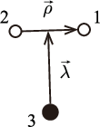
As indicated in Fig. 2, is the relative coordinate between the two light quarks (quark-1 and quark-2), and is the relative coordinate between the center-of-mass of the two light quarks and the charm quark.
The reduced masses and are defined by
| (6) |
and the frequencies of the oscillator for - and -modes are by
| (7) |
Orbital wave functions of the three-quark state are expressed by a simple product of the eigenfunctions of the separated Hamiltonians
| (8) |
where is the total momentum of the three-quark state, and and the wave functions of the Jacobi coordinates and . The wave functions of the harmonic oscillator are given by
| (9) |
where the radial function is summarized in Appendix and is the spherical harmonics. We will call the excitation with either (radial excitation) or (orbital excitation) the -mode. This is also the case for the -mode. When both -mode and -mode happen, this is called the -mode.
The full wave functions of baryons are constructed by products of isospin (flavor) part, spin part, and the orbital part. For the isospin part, we introduce the notation for the two light quarks as
| (10) |
for state, and
| (11) |
for states. The flavor wave function of the baryons having is then expressed by ( stands for the charm quark), and that of the baryons with is by .
Similarly, the spin wave functions of the two light quarks are expressed by ,
| (12) | |||
| (13) |
For the charm quark spin, we use the symbol for either spin up or down.
By making use of these expressions, the full wave functions of the and with total spin are constructed as
| (14) | |||
| (15) |
by anti-symmetrizing the light quark part including the color part which is not explicitly shown here. The total spin of the charmed baryon is given by the sum of the spin of charm quark and the “total” angular momentum of all the remaining part (so-called brown muck [5]) which is obtained by composing the orbital angular momenta and and diquark spin . For example, the wave functions of orbital ground state for the charmed baryons are given by
| (16) | |||
| (17) |
and
| (18) |
| Ground states charmed baryons | |||||
| possible assignment | |||||
| , | |||||
| Negative parity excited charmed baryons | |||||
| possible assignment | |||||
| , | |||||
| (?) | |||||
| Positive parity excited charmed baryons | |||||
| possible assignment | |||||
| (?) | |||||
| (?) | |||||
| Positive parity excited charmed baryons (-mode) | ||||||
| possible assignment | ||||||
| 0 | ||||||
| 1 | ||||||
| (?) | ||||||
| 2 | ||||||
| (?) | ||||||
| (?) | ||||||
In Table 1, we summarize the quark configurations for the charmed baryons considered in this article. The observed excited states and baryons are, due to their small excitation energies, assigned to be the -wave excitations of the -mode (, ) with spin-0 diquark (). Their quark configurations are given by
and
Another possibility to construct the negative parity excited states for is the so-called -mode excitation (, ), which must have the spin-1 diquark () due to the anti-symmetrization of the wave function. The total spin of the brown muck can be , 1 and 2, leading to a HQS singlet with the baryon spin , and two HQS doublets and , respectively. For example, the concrete form for the HQS singlet is given by
The minimal configuration for state for baryons is an orbital excitation for the nodal quantum number or as with spin-0 diquark given by
| (22) | |||||
| (23) |
both of which are the HQS singlets.
The higher excited states of with can be constructed by the -wave excitation as the total angular momentum. In this case, we have three possibilities as , and . In the and cases, the diquark spin should be 0, and the total baryon spin can be , as,
| (24) | |||
In the case with , the diquark spin should be 1 as
The total angular momentum () can be 0, 1 and 2, and the resulting brown muck spin can be , , and giving 13 states. The heavy baryons are the HQS singlet only for and the HQS doublet for the others.
We leave a comment on the difference between the wave function used in Ref. [32] and ours. In Ref. [32], the bases of the quark wave function are given by , namely
| (27) |
while ours are given by
| (28) |
They are different in general except for the highest weight state of and . In the latter, the subcomponent , which is assigned as the brown muck spin , decouples from the heavy quark spin in the heavy quark limit. Hence the latter basis is compatible with the heavy quark symmetry.
III Formulation
III.1 Basic interaction of the pion
In the constituent quark model, the pion can couple to a single quark through the Yukawa interaction, which is considered to contribute dominantly to one-pion emission decays (Fig. 3). In the relativistic description, there are two independent couplings of pseudo-scalar and axial-vector types,
| (29) |
In the non-relativistic model, they correspond to the following two terms,
| (30) |
where is the momentum of the initial (final) quarks and is the pion momentum. We keep in mind that these two couplings in Eq. (29) are equivalent for the on-shell particles in the initial and final states, but not for the off-shell particles confined within a finite size. The present case is the latter, because the quarks are confined in the harmonic oscillator potential. In this work, we employ the axial-vector type coupling,
| (31) |
in accordance with the low-energy chiral dynamics. The non-relativistic limit in Eq. (31) leads to the combination of the two terms in Eq. (29). In Eq. (31), is the axial coupling of the light quarks, for which we use the value [40, 41]. As we will see later, importantly, the axial-vector coupling can explain surprisingly well the decay of through the time-derivative piece in Eq. (31). Contrary, the pseudoscalar coupling cannot reproduce it because it is proportional to the pion momentum which almost vanishes. This strongly supports the chiral dynamics of the pion working with constituent light quarks.
III.2 Matrix elements with the quark model wave functions
In this section, we formulate the one-pion emission decay of a charmed baryon within the quark model. The relevant diagram is shown in Fig. 3, where one pion is emitted from a single light quark. We write state vector for the baryon ( or ) with mass , spin and momentum in the baryon rest frame in the momentum representation as,
| (32) |
which is a superposition of quarks in the momentum space , , and , weighted by the baryon wave functions and . Here the relative momenta and are defined by
| (33) | |||||
| (34) |
and the total momentum of three quarks, which is the baryon momentum, is given by
| (35) |

The factors of are for the normalizations of the confined quark states so that . The sum is taken over the spins of the three quarks and their angular momenta such that the total angular momentum gives the spin .
The decay amplitude for is given by
| (36) |
where only one light quark in the initial and final baryon state participates in the transition as
| (37) |
while the other light quark and the charm quark are spectators and then their matrix elements are just delta-functions of their three-momenta
where or . We have now ten -integrals as
| (39) |
and the first -integral leads to the energy conservation in process. We rewrite the remaining -integrals in terms of the Jacobi coordinates and we find
| (40) |
The -integral leads to the total three-momentum conservation, via . By eliminating the common delta-functions for the energy-momentum conservation, we find the amplitude for decay as
| (41) |
where the effective momentum transfer and appearing in the pion plain wave are defined by
| (42) |
The first term in Eq. (41) involves the relative momenta and of the constituent quarks in the final baryon, which can be replaced by the derivative of the wave functions as
| (43) | |||||
and the same for . In the case of , after performing the momentum integrals and by showing the flavor (isospin) part explicitly, the decay amplitude is given by
| (44) |
where and matrices operate the spin and isospin wave functions of the quark-1. For simplicity, the notation for the bra and ket states
| (45) |
are used in Eq. (44). The derivatives and operate the final state wave functions. We also have to consider the case that the pion couples to the another light quark . Summing over the amplitudes of the two cases coherently, we obtain the total decay amplitude.
III.3 Decay widths with the helicity amplitude
The decay width of is given by
| (46) |
where is the magnitude of the three-momentum of the final pion in the center-of-mass frame, and the sum is taken over the possible quantum numbers, in the present case, the spin state (helicity) of the final baryon for a given initial baryon spin. The matrix element depends on the decay angle (the angle between the quantization axis of the initial baryon spin and the momentum vector of the final baryon) and on the helicity of . In this article, we employ the helicity amplitude approach to calculate the decay width in Eq. (46).
In this approach, we expand the initial spin state , which is quantized along a fixed axis, in the angular momentum basis quantized along the direction of the momentum of the final baryon, , by
| (47) |
where are the Wigner’s functions [42]. If the spin of the final state is quantized along , then the helicity is equal to the third component of the final state spin,
| (48) |
where is the spin of the final baryon .
Hence the matrix element is written with its angular dependence as shown explicitly
| (49) |
where only the diagonal element remains after summing over , because of the helicity (spin -component) conservation. In Eq. (49) both of the initial and final spins are quantized along axis.
Now, the helicity amplitude is defined by
| (50) |
The amplitude depends on , and , but does not depend on the decay angle, because the spin quantization axis is chosen along the direction of the momentum of the final baryon , which is equal to the situation of the decay into the -direction. The possible angular dependence of is taken care of by the function, and the angular-integral in Eq. (46) then can be performed exactly and finally we find
| (51) |
where . Here, the amplitude with the opposite helicity has the same form as .
III.4 Parameters
In the present Hamiltonian of the harmonic oscillator in Eq. (1), we have three model-parameters; the mass of the light quark, that of the heavy quark, and the spring constant. The masses of the quarks are set to be as,
| (52) |
We tune the value of so that the level spacing of the -mode excitation as GeV and the root-mean-square radius of the charmed baryon as 0.45–0.55 fm which is defined as the average of the distance of each quark from the center-of-mass as,
| (53) | |||||
We summarize the model parameters used in the present calculation in Table 2. Depending on these input parameters, the range parameters of the Gaussian wave functions vary within the range of
| (54) |
which is the source of the uncertainty in our theory predictions.
| light quark mass | 0.3–0.4 (GeV) | |
|---|---|---|
| inputs | heavy quark mass | 1.4–1.6 (GeV) |
| H.O. potential | 0.02–0.038 (GeV3) | |
| H.O. energy | 0.3–0.4 (GeV) | |
| outputs | H.O. energy | 0.42–0.58 (GeV) |
| gauss range | 0.36–0.44 (GeV) | |
| gauss range | 0.26–0.32 (GeV) | |
| 0.55–0.67 (fm) | ||
| 0.76–0.93 (fm) | ||
| 0.45–0.55 (fm) |
IV Numerical Results
IV.1 Decays of the ground state and
| (MeV) | (MeV) | (MeV/c) | (MeV) |
|---|---|---|---|
| 1.89 | 89 | 4.27–4.33 | |
| 14.78 | 177 | 30.3–31.6 | |
The baryon is an orbital ground state baryon having . The mass of the is MeV and its full width is (MeV) [25]. The decay channel is the only possible strong decay and its branching ratio is . The baryon has and is expected to form a HQS doublet with . The mass of the is (MeV) and its width is (MeV) [25]. Again the decay channel is the only possible channel in the strong decay and its branching ratio is . Because both and baryons are the spin and isospin flip states of the ground state , their decay rates reflect mainly the spin-isospin structure and is rather insensitive to the spatial structure. Therefore, we can use these processes to check the validity of the present quark model calculations.
The helicity amplitude for the decay is given by,
| (55) |
where and correspond to the term and the term in Eq. (44), respectively. They are given by
| (56) |
and
| (57) |
where and denotes the coupling constant and the normalizations as,
| (58) |
The function denotes the Gaussian form factor as
| (59) |
which is the Fourier transform of ground to ground transition amplitude. The factors of and correspond to the inverse of the range of the Gaussian wave functions for - and -motions, respectively, and their definitions are given in Appendix. Similarly, the helicity amplitude for the decay is given by the same expressions as Eqs. (56) and (57) but the factor is replaced by in both equations.
In Table 3, we show the numerical results for the decay. The calculated decay width is almost twice as large as the experimental value. We also show the results of decay in the same table. The calculated decay width of is again twice as large as the experimental value.
As shown in the table, the uncertainty from the ambiguities of the quark model parameters is small, which means the decay width of the ground state to the ground state does not depend on the detail of the wave functions, as anticipated. Therefore the discrepancy might come from the axial-coupling constant for the interaction.
In the present calculation, we employ for the coupling, but it is also known that this value does not reproduce the axial-coupling constant of the nucleon but leads to instead. To reproduce the axial-coupling constant of the nucleon , one needs a suppression factor of about 3/4 for , which reduces the decay width by a factor , the result of which is consistent with the experimental data. This is expected because the pion emission decays essentially measure the axial couplings for relevant baryons (transitions). Our input here is the axial coupling of the constituent quarks which can take in principle any value when chiral symmetry is spontaneously broken. Here we have shown that it is 3/4 empirically from the phenomena of the ground state baryons not only for the nucleon but also for charmed baryons, which is not far from the discussion of Weinberg [40]. The suppression of has been considered to be originated from the mixing of -waves due to relativistic corrections or pion clouds [43]. This, however, may vary for different baryon excitations. Keeping this in mind, in the following calculations for decays of the excited states, we keep using the value .
IV.2
The baryon is the first excited charmed baryons with and is expected to have . The total decay width is MeV, where the channel is the only strong decay. The seems to be dominated by and its branching ratio is quoted as % [25]. The direct three-body decay width is which we do not calculate in this article.
Employing the quark model, we have three possibilities to describe the excited baryon having as discussed in the previous section. One is the -mode excitation having , and the other two are the -mode excitations having and .
The helicity amplitude for the emission decay of is found again as the sum
| (60) |
where
| (61) |
and
| (62) |
where
| (63) |
which are determined by the Clebsch-Gordan coefficients. We summarize the general expressions in Appendix. We can see that, the starts from reflecting properly the nature of possible -wave decay, while is of order . We will see that the former gives a considerable contribution to the decay width.
As for the -mode with , we find a similar form for the decay as
| (64) |
and
| (65) |
where
| (66) |
In contrast to the above two cases, the situation is quite different for the decay of having the brown muck spin . The amplitudes are exactly zero as,
| (67) | |||
| (68) |
for the decay into baryon. This is due to the spin conservation of the brown muck; the spin-parity state cannot decay into with the pion for any combination of relative angular momentum. Generally, as we will see more examples, such requirements lead to selection rules due to the consistency between the decays of baryons and decays of brown muck, or the diquark in the quark model because the pion couples only to the light quarks. Such observations can be done best by using the baryon wave functions as inspired by the heavy quark symmetry.

To estimate the decay width of the baryon, we should take the finite width of the finial baryon into account, because the threshold is very close to the mass. Indeed, the and channels barely close at the mass while the channel opens, which means the isospin breaking is large contrary to the assumption made in PDG [25]. To this end, we convolute the decay width of by the finite width of as
| (69) |
where is the calculated decay width of given in Eq. (51) which depends on the mass of the final baryon. The normalization factor is defined by,
| (70) |
We take into account the phase space factor for the decay width in the convolution integral as,
| (71) |
where is the mass of the ground state , and is the decay width of given by (MeV) for , (MeV) for . Because only the upper limit is determined for , we calculate the ratio of by employing our formalism discussed in Sec. IV.1, and then estimate it as (MeV) for . The convolution corresponds to the consideration of the sequential decay of the followed by as depicted in Fig. 4. The double emission decay of can be approximated by the convoluted single decay of (including a symmetry factor for the two identical particles), because of the dominant contribution of the on-shell [28]. Similarly, the charged pion decay is approximated by the sum of the and decays.

| decay width ( (MeV)) | |||||||
| decay channel | full | ||||||
| Experimental value (MeV) [25] | - | 0.624 (24%) | 0.624 (24%) | - | |||
| momentum of final particle (MeV/c) | - | - | 29 | ||||
| this work | , | ||||||
| , | 1.5–2.9 | 0.13–0.25 | 0.15–0.28 | 1.2–2.4 | |||
| (MeV) | , | 0 | 0 | 0 | 0 | ||
| 6.5–11.9 | 0.57–1.04 | 0.63–1.15 | 5.3–9.7 | ||||
| (MeV) | 2453.97 | 2453.75 | 2452.9 | ||||
| input parameters employed | (MeV) | 1.89 | 1.83 | 2.1 | |||
| in the convolution Eq. (69) | (MeV) | 139.57 | 139.57 | 134.98 | |||
In Fig. 5, we show the calculated result for the decay width of the baryon in the case of the -mode as functions of the mass of the (the total energy ). We find that the decay width remains finite even at which is below the threshold, owing to the finite width of the baryon. We can also see that the threshold is located at 5 MeV below and then the decay width is much larger than that of , meaning a large isospin breaking. We also show the resulting Breit-Wigner form in Fig. 5 with the fixed width at (MeV) and with the energy-dependent width. In the present case, both of the BW functions resemble because of the resulting small width. However, the energy-dependence of the width is large, so we have to be careful when estimating the BW width for .
In Table 4 we show the calculated decay widths of , , and together with the sum of these three channels evaluated at (MeV). These numbers have uncertainty reflecting that of model parameters of as discussed in Sec. III.4. The uncertainty of the model parameters leads to almost factor-two difference in the decay widths. In spite of this uncertainty including the one coming from , using the axial-vector coupling works well to reproduce the relatively large decay width of located at almost threshold. This is due to the time derivative term with the strength determined the mass of the pion. Thus the decay of provides a good example to show that the chiral theory works up to the order . As discussed in the previous section, we find that, by employing the pseudo-scalar coupling () for the pion, we obtain less than 1 (keV) for the decay due to the small pion momentum .
We also find that the assignment of the -mode configuration with to the leads to almost 2.5 – 5 times larger width than the experimental value for the total width. They are significantly large even if we consider the uncertainty of the pion coupling, because the experimental total width contains not only the decay channel but also the non-resonant three-body decay of which we do not consider in this paper.
In addition, the -mode configuration with cannot decay into . Therefore we can conclude that, by the detailed study of decay width, it is likely that baryon is dominated by the -mode configuration as expected. We might add a comment that other assignments of the or higher spin configurations for cannot reproduce the large experimental value for the decay width due to -wave (or higher partial wave) nature.
IV.3
| decay width ( (MeV)) | ||||
| decay channel | full | |||
| Experimental value (MeV) [25] | ||||
| momentum of final particle (MeV/c) | - | 101 | ||
| this work | , | |||
| , | 5.4–10.7 | |||
| (MeV) | 0.024–0.039 | |||
| , | 0 | |||
| 24.0–45.1 | ||||
| 0.013–0.019 | ||||
| 0.023–0.034 | ||||
| 0.010–0.015 | ||||
The baryon is very narrow resonant state and is expected to have . In PDG, only the upper limit of the decay width is given as MeV [25]. The and its submode are the only strong decay channel. The branching ratio is less than 5%, and therefore the partial decay width for is less than 0.05 MeV.
As discussed in the previous section, the baryon is assigned to be the low-lying orbital excitation state with with spin-0 light diquark. The helicity amplitude for the is then given by the same expressions as Eqs. (61) and (62) but with the different coefficients as
| (72) |
In contrast to the case of , the coefficient of the term is zero then the helicity amplitudes and are of order of as expected for the decay.
We have two more possible quark configurations for the excitations with , which are the -mode excitations with and . The helicity amplitudes for these configurations are found to be again the same as Eqs. (64) and (65) but with different coefficients as
| (73) |
for decay, and
| (74) |
for decay.
In Table 5 we show the numerical results for the decay. In the case, we do not convolute over the finite width of because the threshold is well below the mass, and the convolution does not change the result much. In the table, we also show the calculated decay widths of other assignments than .
We find that the assignment of -mode configuration with for works very well to describe the small decay width of the , while the assignment of leads to larger width than the experimental value. In contrast to the case of , however, we cannot exclude the possibilities of the -mode configurations for by the study of decay width, because the calculated decay widths for -mode and two -modes with are accidentally similar to each other. It is interesting, however, that these three modes give quite different transition amplitudes for the decay as will be discussed later in Sec. IV.4, although the channel is closed for . To discuss the structure of in more detail, we need systematical analyses of the mass spectrum [24], non-resonant three-body decay, and so on.
| decay width ( (MeV)) | |||||||
|---|---|---|---|---|---|---|---|
| decay channel | full | ||||||
| Experimental value (MeV) | 50 [25] | - | - | - | |||
| momentum of final particle (MeV/c) | 265 | 197 | |||||
| , | |||||||
| , | 65.1–146.3 | 61.2–140.2 | 3.9–6.1 | 0.044–0.064 | |||
| 52.2–104.2 | 7.9–11.9 | 44.3–92.4 | 5.6–7.8 | ||||
| , | 0 | 0 | 0 | - | |||
| this work | 325.8–676.3 | 323.7–673.3 | 2.1–3.0 | 0.0044–0.0064 | |||
| 210.4–413.5 | 4.2–5.8 | 206.2–407.7 | 49–70 | ||||
| (MeV) | 9.4–13.1 | 7.6–10.5 | 1.9–2.7 | 0.25–0.26 | |||
| 6.3–8.8 | 3.4–4.7 | 2.9–4.2 | 0.87–0.90 | ||||
| , | 1.6–4.5 | 0.86–2.49 | 0.78–1.98 | 0.79–0.91 | |||
| , | 4.7–10.9 | 4.4–10.1 | 0.33–0.72 | 0.071–0.076 | |||
| 1.9–4.4 | 0.13–0.32 | 1.77–4.04 | 12.8–13.8 | ||||
IV.4 Decays of the higher excited baryons
In Ref. [25], three more states are nominated, , , and , though cannot be excluded for . Among them, spin of is the only quantum number that is well determined in experiment. The parity of is assigned to be positive, but it deserves being carefully examined. Therefore we consider possible assignments of both positive and negative parity cases. For these higher states, the channel opens in addition to the channel. The ratio of also can help us to determine the quantum numbers, and the quark configuration as well. In the following discussions, denotes with or with .
IV.4.1 decay
The baryon is seen in channel as a broad peak [25, 44]. The width is reported as (MeV), but its quantum numbers are still unknown. For this baryon, we consider the -wave excitations in - or -mode with negative parity; or . We also consider the possibility of -wave or -wave excitations in -mode with positive parity; or . Further studies on with other quark configurations are in progress and will be discussed elsewhere [45].
In Table 6, we summarize the possible spin-parity considered here together with the calculated results. Because the partial decay widths are not measured yet, we show the isospin summed width calculated by using the isospin-averaged masses and . The concrete forms of the helicity amplitudes are summarized in Appendix. We find that, for higher , the decay width tends to be smaller due to the suppression of the phase space for higher relative angular momentum in the final state.
| decay width ( (MeV)) | |||||||
|---|---|---|---|---|---|---|---|
| decay channel | full | ||||||
| Experimental value (MeV) | [25] | 0.225 [39] | |||||
| momentum of final particle (MeV/c) | 375 | 315 | |||||
| , | |||||||
| , | 111.9–254.8 | 76.9–204.0 | 35.0–50.8 | 0.25–0.46 | |||
| 129.6–248.8 | 37.7–52.1 | 91.9–196.7 | 2.4–3.8 | ||||
| , | 0 | 0 | 0 | - | |||
| this work | 502.5–1129.7 | 483.9–1104.7 | 18.6–24.9 | 0.038–0.023 | |||
| 439.3–919.5 | 20.0–25.6 | 419.3–893.9 | 21–35 | ||||
| (MeV) | 52.8–68.5 | 36.0–46.0 | 16.7–22.4 | 0.46–0.49 | |||
| 42.0–55.3 | 16.0–20.5 | 26.0–34.9 | 1.6–1.7 | ||||
| , | 3.7–13.5 | 1.3–5.6 | 2.4–7.9 | 1.4–1.8 | |||
| , | 16.3–39.5 | 13.9–34.2 | 2.4–5.3 | 0.16–0.17 | |||
| 11.2–26.1 | 1.2–2.8 | 9.9–23.3 | 8.1–8.4 | ||||
| , | 16.5–40.2 | 7.0–18.2 | 9.5–22.1 | 1.2–1.4 | |||
| , | 44.8–85.4 | 39.5–76.0 | 5.3–9.4 | 0.12–0.13 | |||
| 27.8–52.2 | 1.4–2.6 | 26.4–49.5 | 18.7–18.9 | ||||
| , | |||||||
| , | 51.7–109.6 | 1.8–3.5 | 49.9–106.1 | 27.5–30.1 | |||
| 0.63–1.68 | 0 | 0.63–1.68 | |||||
| 2.9–5.8 | 2.1–4.0 | 0.85–1.73 | 0.41–0.43 | ||||
In the last column in Table 6, we also show the ratio of the decay widths to and defined by
| (75) |
We find the order of magnitudes of the ratio are quite different for different configurations even if the spin-parity is the same, e.g. , and . In fact, these three modes give the similar widths for the decay as discussed in the previous section, but give quite different widths for . In principle, the baryon can decay by -wave to , while it decays by -wave to . Then the ratio can be expressed by
| (76) |
which is, in general, larger than unity. This is the case for the as
| (77) | |||||
| (78) |
In contrast, the brown muck state cannot decay by -wave to the brown muck state in because of the spin-parity conservation. This is another example of the selection rules in the heavy quark limit. Due to the absence of -wave contribution, the ratio is smaller than unity for as
| (79) |
In this configuration, the amplitudes of and decays are the same except the momentum of pion as discussed in Ref. [4]. Here, we stress that the -wave suppression for is found only in the case of , and not in the other quark configurations. This is the same phenomenon that the state cannot decay into as mentioned in Sec. IV.2, and also is seen for the decay of the as discussed in the next section.
As for the magnitude of the decay width, we find that the assignments of and () give rather large decay widths due to the -wave nature into either or . We can exclude these assignments because the resulting decay widths are too large. Calculated widths for -modes () are slightly larger as compared with the observed full width, which does not seem inconsistent if we consider the uncertainty of . However, by taking into account contributions of decays into non-resonant three-body , these -mode states will receive a larger full width, with which the possibility for them to be identified with might decrease.
Among the considered assignments in this article, the other assignments , , , , and cannot be excluded because the total decay width is consistent with the experimental value. The ratio , however, takes different value reflecting the structure of the baryon which will help to determine the quantum numbers.
IV.4.2 decay
The charmed baryon is observed in channel [39, 44] as well as in channel [46]. The spin is determined as from the angular distribution of the decay into [39]. In PDG [25], the parity is assigned to be positive from the analysis of branching ratio in comparison with the prediction of the chiral perturbation [31] with the heavy quark symmetry [4]. However, as discussed in [31] a subtlety arises when calculating the ratio.
In Table 7 we summarize the quark configurations considered here for . By comparing the observed full width MeV and calculated total one-pion decay width, we can exclude all of the -wave configurations with the negative parity including . As for with -mode excitation, both of the decays and ( in terms of the brown muck) go through by -wave, and the ratio is larger than unity as,
| (80) |
which does not agree with the experimental value [39]. This conclusion is consistent with the chiral perturbation calculation with heavy quark symmetry [31, 4].
| decay width ( (MeV)) | |||||||
|---|---|---|---|---|---|---|---|
| decay channel | full | ||||||
| Experimental value (MeV) | [25] | (seen) | - | ||||
| momentum of final particle (MeV/c) | 427 | 369 | |||||
| , | |||||||
| , | 144.8–313.8 | 73.8–215.4 | 71.0–98.4 | 0.46–0.96 | |||
| 182.2–332.0 | 65.4–85.7 | 116.8–246.3 | 1.8–2.9 | ||||
| , | |||||||
| this work | 557.0–1299.3 | 519.3–1250.9 | 37.6–48.3 | 0.039–0.072 | |||
| 536.5–1152.9 | 34.6–42.2 | 501.8–1110.7 | 15–26 | ||||
| (MeV) | 96.2–119.4 | 62.3–75.9 | 33.9–43.5 | 0.54–0.57 | |||
| 80.4–101.4 | 27.7–33.7 | 52.7–67.7 | 1.9–2.0 | ||||
| , | 3.7–17.4 | 1.1–6.4 | 2.7–11.0 | 1.7–2.5 | |||
| , | 24.9–61.7 | 20.1–51.0 | 4.8–10.8 | 0.21–0.24 | |||
| 19.8–46.6 | 2.8–5.9 | 17.1–40.7 | 6.2–6.9 | ||||
| , | |||||||
| , | 5.8–11.1 | 2.6–4.8 | 3.2–6.2 | 1.22–1.29 | |||
For the spin-parity case, we can consider five configurations as shown in Table 7; one -wave excitation in -motion ( with , denoted by ), the one in -motion ( with , denoted by ), and three double--wave excitations in - and -motions (, , where with , denoted by ). Some of these configurations give consistent decay width with the observed full width (MeV). As for the ratio, however, we obtain considerably different values for different configurations like,
| (81) |
where the ambiguities of model parameters are almost canceled. Note that for state is due to the zero decay width into . Among these five configurations, we find that only one configuration with the brown muck spin with agrees both with the small ratio and with the magnitude of total decay width. This seems to contrast with the calculation in Ref. [31], where the other quark configuration for also gives the small .
This discrepancy can be explained as follows. The decay of goes through only by the -wave in the final two-body state, while the decay can go through both by and -waves. The discussion based on the heavy quark limit leading to the model independent relation is possible only when the same -waves are taken, which is completely contaminated by the presence of the -wave contribution. As shown explicitly in Appendix, the amplitude for can contain the -wave contribution ( term in Eq. (94)). Thus we have
| (82) |
except the case of . Only for the case of , -wave contribution ( term in Eq. (95)) is zero because of the conservation of the brown muck spin-parity; the brown muck of cannot decay into with the pion in -wave, which leads to
| (83) |
We stress here again that the -wave suppression is found only in the case of with , and not in the other states with . Here it is worth to mention that the contribution, which allows us to distinguish the possible quark configurations for the same spin-parity, appears only in term arising from the axial-vector coupling of the pion.
If is assigned as a -mode state, a question arises where the -mode states with are. Excitation energies of the -mode states are expected to be lower than those of the -mode states. Other information such as production rates as discussed in Ref. [47] is helpful to solve this problem, for which an experimental measurement is planned in J-PARC [48].
IV.4.3 decay
As for , a narrow peak is observed both in channel [46] and in channel [39]. The total width is (MeV) [25]. The spin-parity is not determined.
In Table 8, we show the calculated one-pion decay widths together with the considered quark configurations for . In the previous section, we pointed out the possibility that is excitation. If this is the case, a new question arises; which baryon is the partner of the HQS doublet possessing . To discuss the possibility of being the doublet partner of , we also show the one-pion decay width with the assignment for in the last line of Table 8. We can see that this assignment can be consistent with the experimental full width in [25] in the sense that the calculated total one-pion emission decay width does not exceed the reported full width. For the same reason, the negative parity assignments can be excluded for the . Similarly to other baryons, the partial decay widths and/or the ratio will help to determine the quantum numbers and the possible quark configuration as well.
V Summary
We have systematically evaluated the decay widths of the charmed baryons , , , , and into and , as well as and into within the non-relativistic quark model. We have emphasized the usefulness of working in the baryon wave functions constructed to be consistent with heavy quark symmetry. This provides various selection rules associated with the pion emission between brown muck of the baryons. Our findings are as follows:
- •
For the low-lying and baryons the quark model descriptions as the -mode excitations with spin-0 diquark can explain the decay properties very well.
- •
The derivative coupling derived from the axial-vector interaction of is essentially important to produce the experimental decay rate of .
- •
Only one quark configuration for among the possible five configurations can lead to the consistent result with the experimental data, while all other four configurations of cannot if the -wave is properly considered. We note that the HQS does not necessarily lead to the small decay ratio of for . This fact calls an attention to the discussion based on the HQS [4, 31] which requires decays in only one partial wave.
- •
Having the above conclusion, we have discussed the possibility of being the HQS doublet partner of possessing . Here we emphasize that our results concerning the possible HQS doublet, and , can be reached with coupling scheme which respects the heavy quark symmetry.
- •
The ratios of are considerably different for different quark configurations even if the baryon spin-parity is the same. This fact is particularly useful to know the structure of charmed baryons.
In this study, we have discussed the various constraints for the one-pion emission decays due to the selection rules associated with the brown muck spin conservation. We have to keep it in mind, however, that there is still small breaking of heavy quark symmetry for charm quark. The study along this line will be left for future works.
In our discussions in the quark model, we have considered only the excitations of valence quarks. We expect that they provide a good description for low lying states. For higher excitations, however, there may be other modes such as pair creations of quark and anti-quark, gluon excitations and so on. The former can be taken into account in the quark model by couplings to mesons or by an unquenched configurations [49], and in effective hadron models by hadronic molecule configurations [50, 51]. The present systematic studies will help us to know where and how these configurations beyond the quark model ones show up which should be studied in the future J-PARC experiments.
acknowledgment
The authors are grateful to K. Tanida and T. Yoshida for various discussions. This work is supported by Grants-in-Aid for Scientific Research (Grants No. JP26400275(C) for H. Nagahiro), (Grants No. JP15K17641 for S. Y.), (Grants No. JP26400273(C) for A. H.), (Grants No. JP16H02188(A) for H. Noumi) and (Grants No. JP25247036(A) for M. O., S. Y. and A. H.).
Appendix A Harmonic oscillator wave functions
The radial functions are given as,
| (84) | |||||
| (85) | |||||
| (86) | |||||
| (87) |
where
| (88) |
The is either or . The reduced masses of and are defined in Eq. (6).
Appendix B Matrix elements
In this Appendix, we summerize the concrete forms of the helicity amplitudes .
B.1 Ground state decays
The amplitudes for the decays of are given by
| (89) |
where the coefficent is given as
| (90) |
The factor denotes the coupling constant and the normalizations as,
| (91) |
and the function denotes the gaussian form factor as
| (92) |
B.2 Negative parity decays
The amplitudes for the decays of the negative parity excitations with -wave of are given by
| (93) |
where the coefficients and are summarized in Table 9. The subscript is either or , depending on the - or -mode excitations.
| -mode excitation () | |||||
| , | 1/2 | ||||
| 1/2 | 0 | ||||
| 1/2 | 0 | ||||
| 1/2 | |||||
| 3/2 | 0 | ||||
| -mode exciation () | |||||
| , | 1/2 | 0 | 0 | ||
| 1/2 | 0 | 0 | |||
| 1/2 | 2 | ||||
| 1/2 | 0 | ||||
| 1/2 | 0 | ||||
| 1/2 | 2 | ||||
| 3/2 | 2 | ||||
| 1/2 | 0 | ||||
| 1/2 | 0 | ||||
| 3/2 | 0 | ||||
| 1/2 | 0 | ||||
| 1/2 | 0 | ||||
| 3/2 | 0 | ||||
B.3 Positive parity decays
| -mode excitation () | |||||
|---|---|---|---|---|---|
| , | 1/2 | ||||
| 1/2 | |||||
| , | 1/2 | ||||
| 1/2 | |||||
| 3/2 | 0 | ||||
| 1/2 | 0 | ||||
| 1/2 | |||||
| 3/2 | 0 | ||||
| -mode excitation () | |||||
| , | 1/2 | ||||
| 1/2 | |||||
| , | 1/2 | ||||
| 1/2 | |||||
| 3/2 | 0 | ||||
| 1/2 | 0 | ||||
| 1/2 | |||||
| 3/2 | 0 | ||||
The amplitudes for the decays of the positive parity excitations with -wave () or -wave () of are given by
| (94) |
where the coefficients and are summarized in Table 10. The subscript is either or , depending on the - or -mode excitations.
| - mixed excitation | ||||||
| , | 2 | 1/2 | 0 | |||
| 1/2 | ||||||
| 3/2 | ||||||
| 1 | 1/2 | 0 | 0 | |||
| 1/2 | 0 | |||||
| 3/2 | 0 | |||||
| 2 | 1/2 | 0 | ||||
| 1/2 | 0 | |||||
| 3/2 | 0 | |||||
| 2 | 1/2 | 0 | ||||
| 1/2 | 0 | |||||
| 3/2 | 0 | |||||
The amplitudes for the decays of the positive parity excitations with - mixed excited states of are given by
| (95) |
where denotes the total angular momentum and the coefficients and are summarized in Table 11.
Appendix C Matrix elements in the heavy quark limit
In this appendix, we derive the matrix elements in the heavy quark limit to show how and when the geometric factor is separated, leading to the model independent relations [4]. Let us consider one pion emission of a heavy baryon containing one heavy quark and a pair of light quarks . Following the notation in this paper, let the initial baryon denoted by and the final one by . Then the spin and angular momentum couplings for the initial and final states are
| (96) |
where is the baryon spin, the brown muck (light degrees of freedom) total spin, the relative angular momentum of , and is the total spin . The decay probability is then computed as
| (97) |
where is the pion-quark interaction, and the sum over final state is taken over possible ’s. For instance, for the decay of , the angular momentum can be both 1 (-wave) and 3 (-wave), while for the decay of , only -wave is possible.
In the literature, the model independent relation has been discussed for the ratio of the decays into and into . In the heavy quark limit it can be obtained only for the decay into the same and single partial wave . As we have discussed in IV.4 in detail, this is possible only in some limited cases where a selection rule due to the diquark transitions imposes an additional constraint. For a single , after recouping the final state, we obtain the matrix element as follows,
| (101) | |||||
Because the interaction is active only for the light quarks, after the application of the Wigner-Eckart theorem, the matrix element in the third line can be factorized into the one of the light degrees of freedom, , and the trivial one of the heavy quark. If, furthermore, the brown muck configuration is uniquely determined, which is to fix at a single value, the dependence is completely dictated by the 6- symbol and the normalization . This explains how and when the ratio in Eq. (75) can be determined in a model independent manner by the formula (101).
References
- [1] S. Weinberg, Phys. Rev. 130, 776 (1963).
- [2] S. Weinberg, Phys. Rev. 137, B672 (1965).
- [3] H. Nagahiro and A. Hosaka, Phys. Rev. C90, 065201 (2014), arXiv:1406.3684 [hep-ph] .
- [4] N. Isgur and M. B. Wise, Phys. Rev. Lett. 66, 1130 (1991).
- [5] M. Neubert, Phys. Rept. 245, 259 (1994).
- [6] S. Yasui and K. Sudoh, Phys. Rev. D80, 034008 (2009), arXiv:0906.1452 [hep-ph] .
- [7] Y. Yamaguchi, S. Ohkoda, S. Yasui, and A. Hosaka, Phys. Rev. D85, 054003 (2012), arXiv:1111.2691 [hep-ph] .
- [8] Y. Yamaguchi, S. Ohkoda, S. Yasui, and A. Hosaka, Phys. Rev. D84, 014032 (2011), arXiv:1105.0734 [hep-ph] .
- [9] Y. Yamaguchi, S. Yasui, and A. Hosaka, Nucl. Phys. A927, 110 (2014), arXiv:1309.4324 [nucl-th] .
- [10] C. Garcia-Recio, V. K. Magas, T. Mizutani, J. Nieves, A. Ramos, L. L. Salcedo, and L. Tolos, Phys. Rev. D79, 054004 (2009), arXiv:0807.2969 [hep-ph] .
- [11] D. Gamermann, C. Garcia-Recio, J. Nieves, L. L. Salcedo, and L. Tolos, Phys. Rev. D81, 094016 (2010), arXiv:1002.2763 [hep-ph] .
- [12] C. Garcia-Recio, J. Nieves, O. Romanets, L. L. Salcedo, and L. Tolos, Phys. Rev. D87, 034032 (2013), arXiv:1210.4755 [hep-ph] .
- [13] Y. Yamaguchi, S. Ohkoda, A. Hosaka, T. Hyodo, and S. Yasui, Phys. Rev. D91, 034034 (2015), arXiv:1402.5222 [hep-ph] .
- [14] Y.-R. Liu and M. Oka, Phys. Rev. D85, 014015 (2012), arXiv:1103.4624 [hep-ph] .
- [15] S. Maeda, M. Oka, A. Yokota, E. Hiyama, and Y.-R. Liu, PTEP 2016, 023D02 (2016), arXiv:1509.02445 [nucl-th] .
- [16] S. Yasui, K. Sudoh, Y. Yamaguchi, S. Ohkoda, A. Hosaka, and T. Hyodo, Phys. Lett. B727, 185 (2013), arXiv:1304.5293 [hep-ph] .
- [17] S. Yasui and K. Sudoh, Phys. Rev. C87, 015202 (2013), arXiv:1207.3134 [hep-ph] .
- [18] S. Yasui and K. Sudoh, Phys. Rev. C89, 015201 (2014), arXiv:1308.0098 [hep-ph] .
- [19] S. Yasui, Phys. Rev. D91, 014031 (2015), arXiv:1408.3703 [hep-ph] .
- [20] D. Suenaga, B.-R. He, Y.-L. Ma, and M. Harada, Phys. Rev. C89, 068201 (2014), arXiv:1403.5140 [hep-ph] .
- [21] D. Suenaga, B.-R. He, Y.-L. Ma, and M. Harada, Phys. Rev. D91, 036001 (2015), arXiv:1412.2462 [hep-ph] .
- [22] D. Suenaga and M. Harada, Phys. Rev. D93, 076005 (2016), arXiv:1509.08578 [hep-ph] .
- [23] A. Hosaka, T. Hyodo, K. Sudoh, Y. Yamaguchi, and S. Yasui, (2016), arXiv:1606.08685 [hep-ph] .
- [24] T. Yoshida, E. Hiyama, A. Hosaka, M. Oka, and K. Sadato, Phys. Rev. D92, 114029 (2015), arXiv:1510.01067 [hep-ph] .
- [25] K. A. Olive et al. (Particle Data Group), Chin. Phys. C38, 090001 (2014).
- [26] T.-M. Yan, H.-Y. Cheng, C.-Y. Cheung, G.-L. Lin, Y. C. Lin, and H.-L. Yu, Phys. Rev. D46, 1148 (1992), [Erratum: Phys. Rev.D55,5851(1997)].
- [27] P. L. Cho, Phys. Lett. B285, 145 (1992), arXiv:hep-ph/9203225 [hep-ph] .
- [28] P. L. Cho, Phys. Rev. D50, 3295 (1994), arXiv:hep-ph/9401276 [hep-ph] .
- [29] J. L. Rosner, Phys. Rev. D52, 6461 (1995), arXiv:hep-ph/9508252 [hep-ph] .
- [30] C. Albertus, E. Hernandez, J. Nieves, and J. M. Verde-Velasco, Phys. Rev. D72, 094022 (2005), arXiv:hep-ph/0507256 [hep-ph] .
- [31] H.-Y. Cheng and C.-K. Chua, Phys. Rev. D75, 014006 (2007), arXiv:hep-ph/0610283 [hep-ph] .
- [32] X.-H. Zhong and Q. Zhao, Phys. Rev. D77, 074008 (2008), arXiv:0711.4645 [hep-ph] .
- [33] L. A. Copley, N. Isgur, and G. Karl, Phys. Rev. D 20, 768 (1979).
- [34] D. Pirjol and T.-M. Yan, Phys. Rev. D56, 5483 (1997), arXiv:hep-ph/9701291 [hep-ph] .
- [35] H. Albrecht et al. (ARGUS), Phys. Lett. B317, 227 (1993).
- [36] K. W. Edwards et al. (CLEO), Phys. Rev. Lett. 74, 3331 (1995).
- [37] T. Aaltonen et al. (CDF), Phys. Rev. D84, 012003 (2011), arXiv:1105.5995 [hep-ex] .
- [38] P. L. Frabetti et al. (E687), Phys. Rev. Lett. 72, 961 (1994).
- [39] K. Abe et al. (Belle), Proceedings of the 33rd International Conference on High Energy Physics (ICHEP ’06), Phys. Rev. Lett. 98, 262001 (2007), arXiv:hep-ex/0608043 [hep-ex] .
- [40] S. Weinberg, Phys. Rev. Lett. 65, 1181 (1990).
- [41] S. Weinberg, Phys. Rev. Lett. 67, 3473 (1991).
- [42] M. A. Morrison and G. A. Parker, Aust. J. Phys. , 465 (1987).
- [43] A. Chodos, R. L. Jaffe, K. Johnson, and C. B. Thorn, Phys. Rev. D10, 2599 (1974).
- [44] M. Artuso et al. (CLEO), Phys. Rev. Lett. 86, 4479 (2001), arXiv:hep-ex/0010080 [hep-ex] .
- [45] H. Nagahiro and A. Hosaka, in progress.
- [46] B. Aubert et al. (BaBar), Phys. Rev. Lett. 98, 012001 (2007), arXiv:hep-ex/0603052 [hep-ex] .
- [47] S.-H. Kim, A. Hosaka, H.-C. Kim, H. Noumi, and K. Shirotori, Prog. Theor. Exp. Phys. 2014, 103D01 (2014), arXiv:1405.3445 [hep-ph] .
- [48] H. Noumi et al., http://www.j-parc.jp/researcher/Hadron/en/Proposal_e.html#1301 (2012), J-PARC E50 proposal.
- [49] R. Bijker, J. Ferretti, and E. Santopinto, Phys. Rev. C85, 035204 (2012).
- [50] T. Mizutani and A. Ramos, Phys. Rev. C74, 065201 (2006), arXiv:hep-ph/0607257 [hep-ph] .
- [51] J. Haidenbauer, G. Krein, U.-G. Meissner, and L. Tolos, Eur. Phys. J. A47, 18 (2011), arXiv:1008.3794 [nucl-th] .