Combining SOS and Moment Relaxations with Branch and Bound to Extract Solutions to Global Polynomial Optimization Problems
Abstract
In this paper, we present a branch and bound algorithm for extracting approximate solutions to Global Polynomial Optimization (GPO) problems with bounded feasible sets. The algorithm is based on a combination of SOS/Moment relaxations and successively bisecting a hyper-rectangle containing the feasible set of the GPO problem. At each iteration, the algorithm makes a comparison between the volume of the hyper-rectangles and their associated lower bounds to the GPO problem obtained by SOS/Moment relaxations to choose and subdivide an existing hyper-rectangle. For any desired accuracy, if we use sufficiently large order of SOS/Moment relaxations, then the algorithm is guaranteed to return a suboptimal point in a certain sense. For a fixed order of SOS/Moment relaxations, the complexity of the algorithm is linear in the number of iterations and polynomial in the number of constrains. We illustrate the effectiveness of the algorithm for a 6-variable, 5-constraint GPO problem for which the ideal generated by the equality constraints is not zero-dimensional - a case where the existing Moment-based approach for extracting the global minimizer might fail.
I Introduction
Global Polynomial Optimization (GPO) is defined as optimization of the form
| (1) | ||||
| subject to | ||||
where , , and are real-valued polynomials in decision variables . As defined in Eq. 1, the GPO problem encompasses many well-studied sub-classes including Linear Programming (LP), Quadratic Programming (QP), Integer Programming (IP), Semidefinite Programming (SDP) and Mixed-Integer Nonlinear Programming (MINLP) [1]. Because of its generalized form, almost any optimization problem can be cast or approximately cast as a GPO, including certain NP-hard problems from economic dispatch [2], optimal power flow [3] and optimal decentralized control [4]. As applied to control theory, GPO can be used for stability analysis of polynomial dynamical systems by, e.g., verifying polytopic invariants as in [5].
Although GPO is NP-hard, there exist a number of heuristics and algorithms that can efficiently solve special cases of GPO. For example, LP [6, 7], QP [8], and SDP all have associated polynomial-time algorithms. More broadly, if the feasible set is convex and the objective function is convex, then barrier functions and descent methods will typically yield a computationally tractable algorithm. When the problem is not convex, there also exist special cases in which the GPO problem is solvable. For example, in [9] the unconstrained problem was solved by parameterizing the critical points of the objective function via Groebner bases. In the special case of , the problem was solved in [10, 11]. In addition, there exist several widely used heuristics which often yield reasonably suboptimal and approximately or exactly feasible solutions to the GPO problem (e.g. [12, 13]), but which we will not discuss here in depth.
If we expand our definition of algorithm to include those with combinatorial complexity but finite termination time, then if the feasible set of the GPO problem is compact and the ideal generated by the equality constraints is radical and zero dimensional (typical for integer programming [14]), then one may use the moment approach to solving sequential Greatest Lower Bound (GLB) problems to obtain an algorithm with finite termination time. Unfortunately, however, it has been shown that the class of problems for which these methods terminate is a strict subset of the general class of GPO problems [15] and furthermore, there are no tractable conditions verifying if the algorithm will terminate or bounds on computational complexity in the case of finite termination. In this paper, however, we take the idea of generating Greatest Lower Bounds and propose an alternative method for extracting approximate solutions that does not require finite convergence and, hence, has polynomial-time complexity.
Let
| (2) |
be the feasible set and be an optimal solution of GPO Problem (1). The Greatest Lower Bound (GLB) problem associated to GPO Problem (1) is defined as
| (3) | ||||
The GLB and GPO problems are closely related, but are not equivalent. For example, it is clear that , where is as defined in Eq. (1). Furthermore, as discussed in Section V, an algorithm which solves the GLB problem with complexity can be combined with Branch and Bound to approximately solve the GPO for any desired level of accuracy with complexity , where we define an approximate solution to the GPO as a point such that and .
Many convex approaches have been applied to solving the GLB problem, all of which are based on parameterizing the cone of polynomials which are positive over the feasible set of the corresponding GPO problem. The most well-known of these approaches are Sum of Squares (SOS) programming [16], and its dual Moment-relaxation problem [17]. Both these approaches are well-studied and have implementations as Matlab toolboxes, including SOSTOOLS [18] and Gloptipoly [19]. These approaches both yield a hierarchy of primal/dual semidefinite programs with an increasing associated sequence of optimal values (SOS) and (Moment) such that if we denote the OBV of the corresponding GPO problem by , then under mild conditions, both sequences satisfy and [20]. Moreover, if the feasible set of GPO Problem (1), , as defined in (2), is nonempty and compact, then there exist bounds on the error of SOS/Moment relaxations which scale as
for constants and that are functions of polynomials , and [21]. The goal of this paper, then, is to combine the SOS and Moment approaches with a branch and bound methodology to create an algorithm for solving the GPO problem and extracting a solution.
Specifically, in Sec. VI, we propose a sequence of branch and bound algorithms, denoted by , such that for any and for a given GPO problem of Form (1) with a bounded feasible set, Algorithm in polynomial-time returns a point that is sub-optimal to the GPO problem in the following sense. If is the sequence of proposed solutions produced by the sequence of algorithms , we show that if the feasible set, , of Problem (1) is bounded, then there exist a sequence of feasible point such that and , where is the OBV of the GPO problem.
The sequence of algorithms can be briefly summarized as follows. Algorithm initializes with hyper-rectangle such that . Then, at iteration , the algorithm forms two new hyper-rectangles by bisecting by its longest edge () and intersecting each of the new hyper-rectangles with to create two new GPO problems. Then, the algorithm computes a GLB estimate of the OBV of the new GPO problem by solving the corresponding ’th-order SOS/Moment relaxations. If denotes the best lower bound to , obtained up to iteration , then is determined to be the existing hyper-rectangle with a smallest volume subject to the constraint that the corresponding GLB is less that , where and are the design parameters. Finally, after certain number of iterations, the algorithm terminates by returning the centroid of the last hyper-rectangle.
In Sec. VII we discuss the complexity of the proposed algorithm by first showing that for any , the feasible set of the ’th order SOS relaxation associated to a branch is completely contained in that of each of its subdivided branches - implying that the lower bounds obtained by both the SOS and Moment relaxation (due to the duality between SOS and Moment methods) are increasing. Of course, at those branches with , these bounds will approach . Next, we show that if the error of the ’th order SOS/Moment relaxations associated to the hyper-rectangles obtained through Algorithm is bounded by , then each of the bisected hyper-rectangles is guaranteed to contain a feasible point that is -suboptimal. Therefore, the feasible set will be reduced in volume as , up to iteration . In other words, the number of iterations necessary to achieve a hyper-rectangle with a longest edge of the length is logarithmic in . Finally, since at each iteration the number of constraints is fixed and the complexity is linear in the number of iterations, we conclude that algorithm is polynomial-time.
II Notation
Let be the set of n-tuples of natural numbers. We use and to denote the symmetric matrices and cone of positive semidefinite matrices of size , respectively. For any , we denote by the hyper-rectangle , where is defined by the positive orthant. We use to denote the set of bounded infinite sequences. For any , let , where . Finally, we denote the ring of multivariate polynomials with real coefficients as [].
III Problem Statement
In this paper, we consider simplified GPO problems of the form:
| (4) | ||||
| subject to |
where . The class of problems in (4) is equivalent to that in (1), where we have simply replaced every constraint with some and . For every problem of Form (4), we define the associated feasible set
In this paper, we assume . Note that given , one may use SOS optimization combined with Positivstellensatz results [22] to determine feasibility of .
Proposed Algorithm In this paper, we propose a GLB and Branch and Bound-based algorithm which, for any given , will return some for which there exists a point such that:
| (5) |
Furthermore itself is -suboptimal in the sense that and .
Before defining this algorithm, however, in the following section, we describe some background on the dual SOS and Moment algorithms for generating approximate solutions of the GLB Problem.
IV Background on Semidefinite Representations of SOS/Moment Relaxations
In this section, we describe two well-known asymptotic algorithms which are known to generate sequences of increasingly accurate suboptimal solutions to the GLB problem - namely the SOS and Moment approaches. Both these methods use Positivstellensatz results which parameterize the set of polynomials which are positive over a given semialgebraic set.
IV-A Sum-of-Squares Polynomials
In this subsection, we briefly define and denote sets of sums of squares of polynomials.
We denote monomials in variables as where . Monomials can be ordered using various orderings on . In this paper, we use the graded lexicographical ordering. This ordering is defined inductively as follows. For , if or and . Denote by the infinite ordered vector of all monomials, where if . Because we have used the graded lexicographical ordering, if we restrict ourselves to the first elements of , then this is the vector of all monomials of degree or less. We denote this truncated vector as and the length of as . Using this definition, it is clear that any polynomial can be represented as for some , where is the degree of .
The vector of monomials can also be combined with positive matrices to completely parameterize the cone of sums-of-squares polynomials. Formally, we can denote the subset of polynomials which are the sum of squares of polynomials as
| (6) |
Clearly any element of is a nonnegative polynomial. Furthermore, if and is of degree , then there exists a positive semidefinite matrix such that
Conversely, any polynomial of this form, with , is SOS. This parametrization of SOS polynomials using positive matrices will allow us to convert the GLB problem to an LMI. However, before defining this LMI approach, we must examine the question of positivity on semialgebraic subsets of .
IV-B Putinar’s Positivstellensatz, Quadratic Modules and the Archimedean Property
Sum-of-Squares polynomials are globally non-negative. In this section, we briefly review Putinar’s positivstellensatz which gives necessary conditions for a polynomial to be positive on the semiaglebraic set where and is compact.
Putinar’s Positivstellensatz uses the which define to deduce a cone of polynomials which are non-negative on . This cone is the quadratic module which we define as follows.
Definition 1
Given a finite collection of polynomials , we define the quadratic module as
and the degree- bounded quadratic module as
Clearly, any polynomial in is non-negative on . Furthermore, since parameterizes and positive matrices parameterize , the constraint can be represented as an LMI. Furthermore, if the module satisfies the Archimedean property, then Putinar’s Positivstellensatz states that any polynomial which is positive on is an element of . That is, parameterizes the cone of polynomials positive on .
A quadratic module is said to be Archimedean if there exists some and such that . We say that is an Archimedean representation of if the associated quadratic module is Archimedean. Note that the Archimedean property is a property of the functions which then define the quadratic module and not a property of . Specifically, if is compact, then there always exists an Archimedean representation of . Specifically, in this case, there exists an such that for all . Now define .
IV-C SOS approach to solving the GLB problem
In this subsection, we briefly describe the use of SOS programming to define a hierarchy of GLB problems.
Consider the GPO Problem (4) where is an Archimedean representation of the feasible set, , with associated quadratic module . We now define the degree-unbounded version of the SOS GLB problem.
| (7) | ||||
Since is Archimedian, it follows that (where is as defined in (4)). Although Problem (7) is convex, for practical implementation we must restrict the degree of the SOS polynomials which parameterize - meaning, we must restrict ourselves to optimization on . This defines a new sequence of GLB problems as
| (8) | ||||
Clearly, for any . Additionally, it was shown in [16] that . Furthermore, it was shown in [20, 21] that bounds on the convergence rate of exist as a function of , and . Finally, the computational complexity of is equivalent to that of a semidefinite program with order scalar variables.
IV-D Moment approach to solving the GLB problem
In this subsection, we briefly describe the Moment approach to solving the GLB problem.
Let denote the set of Borel subsets of and let be the set of finite and signed Borel measures on . The following lemma uses the set of probability measures with support on to provide a necessary and sufficient condition for a polynomial to be positive over .
Lemma 1
Given and integrable over , a polynomial is nonnegative on if and only if for all such that and .
Again, consider GPO Problem (4) with the feasible set . Now, if we define the moment optimization problem
| (9) | ||||
then Lemma 1 implies, using a duality argument, that where is as defined in Problem (4) [17].
Unfortunately, Problem (9) requires us to optimize over the space of measures . However, as yet we have no way of parameterizing these measures or imposing the constraints and . Fortunately, we find that a measure can be parameterized effectively using the moments generated by the measure. That is, any measure has an associated ordered vector of moments, indexed by using monomial as
Furthermore, if and , then for all , where we define , where is the module defined by the in . More significantly, the converse is also true. This means that if we add the constraint to ensure , then we may replace the measure variable by the moment variable , as described. However, this requires us to enforce the constraint for all such that . This constraint, however, can be represented using semidefinite programming [20, 17]. Finally, if , we can enforce the integral constraint of optimization problem (1) as
This allows us to formulate the equivalent GLB problem as
| (10) | ||||
Then and as for the SOS GLB problem, we define a sequence of truncations of the moment GLB problem
| (11) | ||||
where and .
It has been shown that for all and furthermore . Moreover, if the interior of is not empty, then [20]. Note that is an SDP constraint and the number of decision variables is . This implies that the computational complexity of and are similar.
In the following section, we combine the GLB problems defined by the SOS/Moment approach with a Branch and Bound sequence to approximately solve the GPO problem.
V Solving the GPO Problem using SOS, Moments and Branch and Bound
In this section, we show that the following algorithm can be used to solve the GPO problem given a solution to the GLB problem.
The Ideal Branch and Bound Algorithm
At every iteration, we have a hyper-rectangle ;
- 1.
Initialize the algorithm;
- 2.
Bisect ;
- 3.
Compute the Greatest Lower Bound of
(12) - 4.
If , set , otherwise ;
- 5.
Goto 2 ;
At termination, we choose any , which will be accurate within .
Let us examine these steps in more detail.
Initialize the algorithm Since the set is compact, there exists some such that . We may then initialize , where is the vector of all 1’s.
Bisect Bisection of the hypercube occurs along the longest edge. Thus, after iterations, we are guaranteed a two-fold increase in accuracy. As a result, the largest edge of the hypercube diminishes as .
Compute the Greatest Lower bound We assume that our solution to the GLB problem is exact. In this case, we are guaranteed that an optimizing will always lie in .
V-A Complexity of the Ideal Branch and Bound Algorithm
In this subsection, we show that any exact solution to the GLB can be used to solve the GPO problem with arbitrary accuracy in a logarithmic number of steps using the Ideal Branch and Bound algorithm.
Suppose is a GLB Problem of the Form (3) with solution . Define the algorithm as . Further suppose has time-complexity , where is a measure for the size of . In the Ideal Branch and Bound algorithm, if we use to perform Step (3), it is straightforward to show that for any after iterations, if , then and GPO Problem (4) has a minimizer , where depends on the size of and is the number of variables. Now since all the GLB problems defined in Step (3) of the algorithm are of equal size, , the complexity of the Ideal Branch and Bound algorithm for a given , is .
In this section, we considered the ideal case when the GLB can be solved exactly. In the following section we adapt this algorithm to the case when sequential algorithms such as SOS/Moment problems are used to solve the GLB problem. In this case, our approach will also be defined as a sequence of approximation algorithms.
VI Modified Branch and Bound Algorithm
In this section, we present a slightly modified branch and bound algorithm that combined with SOS/Moment relaxations, can approximate the solution to the GPO problem to any desired accuracy, in a certain sense.
The Modified Branch and Bound Algorithm At every iteration, we have an active hyper-rectangle and a set of feasible rectangles each with associated GLB .
- 1.
Initialize the algorithm
- 2.
Bisect
- 3.
Compute the Greatest Lower Bound of
(13) - 4.
If , add to .
- 5.
Set where is the smallest element of .
- 6.
Goto 2
At termination, we choose any , which will be accurate within .
VI-A Problem Definition and SOS/Moment Subroutine
Consider GPO Problem (4) and suppose the corresponding feasible set is nonempty and compact with , for some with associated Archimedean quadratic module .
Before defining the main sequential algorithm , we will define the -order SOS/Moment GLB subroutine, denoted , which calculates the GLB in Step (3) of the Modified Branch and Bound Algorithm.
SOS/Moment Subroutine
Given , define the polynomials . These polynomials are then used to define the modified feasible set as
| (14) | ||||
and the corresponding modified degree- bounded quadratic module as
| (15) | ||||
where . This allows us to formulate and solve the modified -th order SOS GLB problem
| (16) | ||||
and the corresponding dual GLB moment problem as described in the preceeding section. The subroutine returns the value .
VI-B Formal Definition of the Modified Branch and Bound Algorithm,
We now define a sequence of Algorithms such that for any , takes GPO Problem (4) and returns an estimated feasible point .
The Sequence of Algorithms :
In the following, we use the notation to indicate that the algorithm takes value and assigns it to . That is, . In addition parameter represents error tolerance for trimming branches and in Theorem 1 is set by the desired accuracy as . The parameter represents the number of branch and bound loops and in Theorem 1 is set by the desired accuracy as where is the number of variables and is a bound on the radius of the feasible set.
The inputs to the following algorithm are the functions and , the initial hyper-rectangle such that , and the design parameters , . The output is the estimated feasible point, .
Algorithm
input: , , , [].
output: (as an approximate solution to GPO Problem (4)).
Initialize:
While ()
| (17) | ||||
| For from 1 to | |||
Return ;
In the following section we will discuss the complexity and accuracy of the sequence of Algorithms .
VII Convergence and Complexity of
In this section, we first show that for any , the greatest lower bounds obtained by the subroutine increase at each iteration of the Branch and Bound loop. Next we show that for any desired accuracy, there exists a sufficiently large , such that Algorithm returns a proposed solution with that accuracy.
In the following lemma, we use Lemma 3 from the Appendix to show that for any such that , the feasible set of the SOS problem solved in Subroutine is contained in that of Subroutine .
Lemma 2
For any and , let be the modified degree-k bounded quadratic module associated to polynomials , as defined in (15). If , then , for all .
Proof:
For any let and . Since then it is followed from Lemma 3 in the Appendix that there exist such that
Now, if , we will show that . By definition, there exist such that , where . Hence, we can plug in the expression for to get
Clearly . Furthermore, since , , and which implies that . ∎
Now suppose all have degree or less. Then for any and for any hyper-rectangles , if and are the solutions obtained by Subroutines and applied to GPO Problem (4), then Lemma 2 shows that . Now, for a fixed , let and be the design parameters of Algorithm applied to GPO Problem (1). For , let , where is as we defined in iteration of the loop in Algorithm . Using Lemma 2, it is straightforward to show that for .
In the next theorem, we will show that for any given , there exist such that Algorithm applied to GPO Problem (4) will provide a point satisfying (5).
Theorem 1
Proof:
Define to be the set of all possible hyper-rectangles generated by the branching loop of Algorithm (for any ) with number of branches bounded by . The vertices of all elements of clearly lie on a grid with spacings . Therefore, the cardinality is finite and bounded as a function of , and . It has be shown that for any , there exists a such that for any , the solution of Subroutine is accurate with the error tolerance . Now define .
Will now show that Algorithm returns a point with the desired accuracy. First, we show that Algorithm generates exactly nested hyper-rectangles. The proof is by induction on .
For , let , , , , , , , , , and where , , , , and are defined as in iteration of Algorithm .
We use induction on to show that for all :
The base case is trivial. For the inductive step, first note that for all and . The latter is obtained from Lemma 2 and the former is because at each iteration, . Constraint (17) at iteration , implies that
| (18) |
Now we will show that again, Constraint (17) at iteration is satisfied at least by one of and . Suppose this is not true. Then we can write
| (19) | ||||
Now, since , Eq. (19) implies
| (20) | ||||
Using Eq. (20) and Eq. (18) one can write
| (21) | ||||
This contradicts the fact that all , and have accuracy higher than . Therefore, it is clear that both and can be possible choices to be bisected at iteration . This fact, together with the induction hypothesis which certifies that possesses the smallest volume between all the hyper-rectangles obtained up to that iteration, guaranteeing that either or , will be branched at the next iteration. Therefore, the algorithm will generate nested hyper-rectangles.
Now, implies that
| (22) |
Eq. (18) and Eq.(22) together with the fact that imply
| (23) |
Finally, as a special case , one can write:
Now, note that the -accuracy of implies that is feasible. It also can be implied that contains such that . Therefore,
Finally, if is the point return by Algorithm , then based on the definition of , it is implied that after the last iteration , the largest diagonal of the branched hyper-rectangle is less than , hence , as desired. ∎
Theorem 1 ensures that for any accuracy there exists a such that Algorithm returns -approximate solutions to the GPO problem with a logarithmic bound on the number of branching loops. The following corollary shows that these -approximate solutions can themselves approximately satisfy the constraints of the original GPO as follows.
Corollary 1
Proof:
Let be such that any polynomial satisfies . ( Existence of follows from the Lipschitz continuity of polynomials on compact sets.) Choose such that . Let and satisfy the conditions in Thoerem 1. It is straightforward to show that satisfies Eq. (24). ∎
Unfortunately, of course, Theorem 1 does not provide a bound on the size of (although the proof implies an exponential bound).
VIII Numerical Results
Consider the following GPO problem.
| subject to | |||
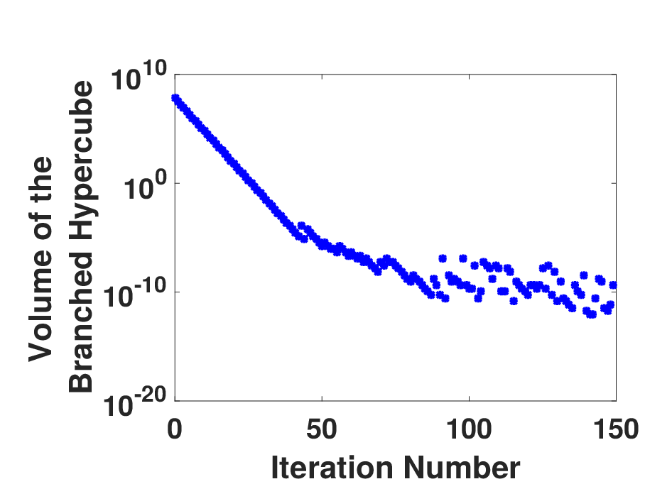
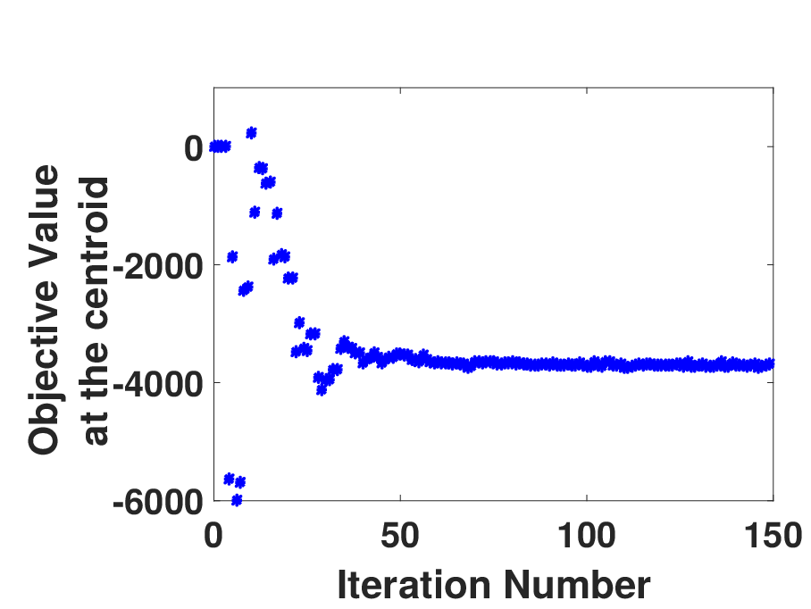
In this example we have 6 variables, an objective function of degree 4 and several equality and inequality constraints of degree 4 or less. The ideal generated by equality constraints is not zero dimensional, hence the Moment approach to extracting solutions fails. We applied Algorithm to this problem with parameters and , using Sedumi to solve the SDPs associated with the SOS and Moment problems. As seen in Figure 1, the branch and bound algorithm converges relatively quickly to a certain level of error and then saturates. Iterations past this point do not significantly improve accuracy of the feasible point. As predicted, this saturation and residual error (blue shaded region) is due the use of a fixed degree bound . As is decreased, the residual error increases and as is increased the residual error decreases. For this problem the final iteration returns the point for which all inequalities are feasible and the equality constraints and have errors of and , respectively. The objective value is .



IX Conclusion
We have proposed a sequence of Algorithms to extract solutions to the GPO problem based on a combination of Branch and Bound and SOS/Moment relaxations. The computational-complexity of Algorithm is polynomial in , polynomial in the number of constraints and linear in the number of branches . Additionally, for any scalar , there exist such that Algorithms , in number of iterations, returns a point that is within the -distance of a feasible and -suboptimal point. For a fixed degree of semidefinite relaxations, our numerical case study demonstrates convergence to a level of residual error which can then be decreased by increasing the degree. In ongoing work, we seek to bound this residual error as a function of degree using available bounds on the error of SOS/Moment relaxations.
The following lemma gives an algebraic property of the polynomials of the form which are used to define the augmented feasible set .
Lemma 3
Let , and . Then, there exist and , such that
Proof:
Without loss of generality, one can assume that (consider the change of variable ). Now let , , and . First, we consider the case where . This leads to two sub-cases:
Case 1 : . Let
and . Verifying the equality is straightforward. To show that , we use the following.
After simplification we have:
which completes the proof for Case 1.
Case 2 : . In this case, let
Equality and positivity for this case can then be easily verified. Now, suppose . In this case, simply set . If , set . The case , is similar to , ,through the change of variable . ∎
References
- [1] M. Laurent, Emerging Applications of Algebraic Geometry, ch. Sums of Squares, Moment Matrices and Optimization Over Polynomials, pp. 157–270. New York, NY: Springer New York, 2009.
- [2] J. B. Park, Y. W. Jeong, J. R. Shin, and K. Y. Lee, “An improved particle swarm optimization for nonconvex economic dispatch problems,” IEEE Transactions on Power Systems, vol. 25, no. 1, pp. 156–166, 2010.
- [3] B. Ghaddar, J. Marecek, and M. Mevissen, “Optimal power flow as a polynomial optimization problem,” IEEE Transactions on Power Systems, vol. 31, no. 1, pp. 539–546, 2016.
- [4] J. Lavaei, “Optimal decentralized control problem as a rank-constrained optimization,” in Communication, Control, and Computing (Allerton), 2013 51st Annual Allerton Conference on, pp. 39–45, IEEE, 2013.
- [5] M. A. B. Sassi and A. Girard, “Computation of polytopic invariants for polynomial dynamical systems using linear programming,” Automatica, vol. 48, no. 12, pp. 3114 – 3121, 2012.
- [6] L. Khachiyan, “Polynomial algorithms in linear programming,” USSR Computational Mathematics and Mathematical Physics, vol. 20, no. 1, pp. 53 – 72, 1980.
- [7] N. Karmarkar, “A new polynomial-time algorithm for linear programming,” Combinatorica, vol. 4, no. 4, pp. 373–395.
- [8] Z.-Q. Luo and S. Zhang, “A semidefinite relaxation scheme for multivariate quartic polynomial optimization with quadratic constraints,” SIAM Journal on Optimization, vol. 20, no. 4, pp. 1716–1736, 2010.
- [9] B. Sturmfels, Solving systems of polynomial equations. No. 97, American Mathematical Soc., 2002.
- [10] H. D. Sherali and C. H. Tuncbilek, “New reformulation linearization/convexification relaxations for univariate and multivariate polynomial programming problems,” Operations Research Letters, vol. 21, no. 1, pp. 1 – 9, 1997.
- [11] N. Z. Shor, “Quadratic optimization problems,” Soviet Journal of Computer and Systems Sciences, vol. 25, no. 6, pp. 1–11, 1987.
- [12] W. Cook, T. Koch, D. E. Steffy, and K. Wolter, “A hybrid branch-and-bound approach for exact rational mixed-integer programming,” Mathematical Programming Computation, vol. 5, no. 3, pp. 305–344, 2013.
- [13] D. E. Steffy and K. Wolter, “Valid linear programming bounds for exact mixed-integer programming,” INFORMS Journal on Computing, vol. 25, no. 2, pp. 271–284, 2013.
- [14] J. Lasserre, “Polynomials nonnegative on a grid and discrete optimization,” Transactions of the American Mathematical Society, vol. 354, no. 2, pp. 631–649, 2002.
- [15] J. Nie, “Optimality conditions and finite convergence of lasserre’s hierarchy,” Mathematical Programming, vol. 146, no. 1, pp. 97–121, 2013.
- [16] P. A. Parrilo, Structured semidefinite programs and semialgebraic geometry methods in robustness and optimization. PhD thesis, Citeseer, 2000.
- [17] J. B. Lasserre, Moments, positive polynomials and their applications, vol. 1. London: World Scientific, 2009.
- [18] S. Prajna, A. Papachristodoulou, and P. A. Parrilo, “Introducing sostools: A general purpose sum of squares programming solver,” in Decision and Control, 2002, Proceedings of the 41st IEEE Conference on, vol. 1, pp. 741–746, IEEE, 2002.
- [19] D. Henrion and J.-B. Lasserre, Positive Polynomials in Control, ch. Detecting Global Optimality and Extracting Solutions in GloptiPoly, pp. 293–310. Berlin, Heidelberg: Springer Berlin Heidelberg, 2005.
- [20] M. Schweighofer, “Optimization of polynomials on compact semialgebraic sets,” SIAM Journal on Optimization, vol. 15, no. 3, pp. 805–825, 2005.
- [21] J. Nie and M. Schweighofer, “On the complexity of putinar’s positivstellensatz,” Journal of Complexity, vol. 23, no. 1, pp. 135 – 150, 2007.
- [22] G. Stengle, “A nullstellensatz and a positivstellensatz in semialgebraic geometry,” Mathematische Annalen, vol. 207, no. 2, pp. 87–97, 1974.