Complexity of quantum impurity problems
Abstract
We give a quasi-polynomial time classical algorithm for estimating the ground state energy and for computing low energy states of quantum impurity models. Such models describe a bath of free fermions coupled to a small interacting subsystem called an impurity. The full system consists of fermionic modes and has a Hamiltonian , where is quadratic in creation-annihilation operators and is an arbitrary Hamiltonian acting on a subset of modes. We show that the ground energy of can be approximated with an additive error in time . Our algorithm also finds a low energy state that achieves this approximation. The low energy state is represented as a superposition of fermionic Gaussian states. To arrive at this result we prove several theorems concerning exact ground states of impurity models. In particular, we show that eigenvalues of the ground state covariance matrix decay exponentially with the exponent depending very mildly on the spectral gap of . A key ingredient of our proof is Zolotarev’s rational approximation to the function. We anticipate that our algorithms may be used in hybrid quantum-classical simulations of strongly correlated materials based on dynamical mean field theory. We implemented a simplified practical version of our algorithm and benchmarked it using the single impurity Anderson model.
1 Introduction
In this paper we study ground states and low energy states of quantum impurity models. Such models describe a bath of free fermions coupled to a small interacting subsystem called an impurity.
Hamiltonians of this form were famously studied in the 1960s and 70s by Anderson, Kondo, Wilson, and many others to investigate the physics of a magnetic impurity embedded in a metal [1, 2, 3]. This line of research elucidated the theoretical mechanism of the Kondo effect11 1 While it is generally expected that a metal should become a better conductor as temperature is reduced, for some metals with dilute impurities the resistivity achieves a minimum value at a nonzero temperature. In short, the resistivity can increase as temperature is lowered due to scattering of conduction electrons in the metal with a localized electron in the impurity (see, e.g., Ref. [4]). which had been observed experimentally decades earlier [5]. It also spurred the development of Wilson’s numerical renormalization group [3], a non-perturbative numerical method which reproduces the low temperature physics of these systems.
The study of quantum impurity models extends beyond this direct application and provides a powerful numerical method for calculating electronic structure of strongly correlated materials such as transition metal compounds and high-temperature superconductors [6]. These materials are described by fermionic lattice models with interactions throughout the system, instead of localized within a small subsystem. Nevertheless, impurity models can be used to study such materials within an approximation known as dynamical mean field theory (DMFT) [7]. The impurity is typically chosen to model a group of atoms contained within a unit cell of the lattice, whereas the bath models the bulk of the material.
Recently there has been growing interest in solving impurity problems in the quantum information community. It was suggested by Bauer et al. [8] that a small quantum computer with a few hundred qubits can potentially speed up certain steps in material simulations based on the DMFT method. In particular, Ref. [8] proposed a quantum algorithm for computing the Green’s function of a quantum impurity model. Kreula et al. [9] subsequently proposed a proof-of-principle demonstration of this algorithm.
Quantum impurity problems are also interesting from the standpoint of Hamiltonian complexity theory [10]. In general, estimating the ground energy of a quantum many-body system composed of spins or fermi modes with local interactions is a hard problem. Formally, this problem is complete for the complexity class QMA – a quantum analogue of NP [11, 12]. The QMA-completeness result implies that, in the worst case, the ground energy of interacting fermi systems cannot be computed efficiently (assuming QMABQP). In contrast, Hamiltonians describing free fermions are exactly solvable and their ground energy can be computed in polynomial time. Quantum impurity models provide a natural arena for studying the complexity of fermionic systems in an intermediate regime interpolating between the free and the fully interacting cases.
In this paper we describe a classical algorithm for approximating the ground energy and for computing low energy states of quantum impurity models. We focus on the worst-case computational complexity of this problem as a function of the system size and the desired approximation error. We also prove several theorems concerning exact ground states of impurity models that appear to be new.
1.1 Main results
To state our results let us first define a general quantum impurity model. We consider the -dimensional Hilbert space of fermi modes, spanned by Fock basis vectors
Here are fermionic creation and annihilation operators, is the occupation number of the th mode and is the vacuum state which satisfies for all . A quantum impurity model is a Hamiltonian which acts on as
where describes a bath of free fermions and describes the impurity. To specify the form of and it will be convenient to use Majorana operators defined by
| (1) |
The Majorana operators are hermitian and satisfy
| (2) |
for all . We may write any free fermion Hamiltonian as
| (3) |
where is real anti-symmetric matrix and is an energy shift chosen such that has zero ground energy. Here and in the following we use to denote the trace norm, while denotes the operator norm. Let us choose the energy scale such that . Then single-particle excitation energies of belong to the interval while eigenvalues of belong to the interval .
Let us agree that acts non-trivially only on the Majorana modes . Here is the impurity size. We shall be interested in the case . The impurity Hamiltonian must include only even-weight Majorana operators (i.e., fermionic parity is conserved) but otherwise can be completely arbitrary. We may write the impurity Hamiltonian as
where are some coefficients22 2 In order for to be hermitian, the coefficients must be real for and imaginary for .. We do not impose any restrictions on the magnitude of these coefficients or on the norm of . Let us write
for the ground energy of the full Hamiltonian. Our main result is as follows.
Theorem 1 (Quasipolynomial algorithm).
There exists a classical algorithm which takes as input a quantum impurity model , a target precision , and outputs an estimate such that . The algorithm has runtime
For a fixed impurity size the runtime is polynomial in and quasi-polynomial in . We are not aware of any obstacles to achieving a polynomial scaling in and leave this as as open problem. On the other hand, the dependence of the runtime on and is nearly optimal. Indeed, choosing and reduces the problem to approximating the ground energy of and respectively. In the worst case this requires time and respectively (using existing methods). As far as we know, our algorithm is the first proposed method which gives a rigorous bound on the approximation error for general impurity models.
The proof of Theorem 1 including a complete description of the algorithm is given in Section 4.2. At a high level the algorithm proceeds as follows. We introduce a deformed impurity problem in which the single-particle energies of the bath Hamiltonian are approximated by a set of equally spaced grid points33 3 We note that a discretization of the bath Hamiltonian is also used in the numerical renormalization group method [3].. This deformed impurity problem has a special feature that a large number of fermionic modes can be decoupled from the impurity by a (Gaussian) unitary transformation. We show that the full Hamiltonian has a low-energy state within a subspace spanned by eigenstates of the deformed bath Hamiltonian such that (a) bath modes coupled to the impurity have at most excitations and (b) all decoupled modes are unoccupied. We show that the dimension of is upper bounded by . Note that the dimension of has no dependence on . We approximate the ground energy by restricting the deformed impurity model onto the subspace and using exact diagonalization to compute the smallest eigenvalue. The corresponding smallest eigenvector can be written as a superposition of at most fermionic Gaussian states.
The analysis of our algorithm relies on new results concerning ground states of quantum impurity models; in particular, Theorem 2 (described below) and its corollaries. A simplified practical version of our algorithm is described in Section 5 and benchmarked using the single impurity Anderson model [1].
Remark: The runtime quoted in theorem 1 counts the total number of elementary algebraic operations . Moreover, for the sake of readability, throughout the paper we ignore errors incurred in the standard linear algebra subroutines. In particular, we assume that eigenvalues of a hermitian matrix can be computed exactly in time . Strictly speaking, the cost of this computation has a mild dependence on the desired precision and the norm of . Applying Householder transformations to make tri-diagonal and using rigorous eigenvalue algorithms for tri-diagonal matrices [13] one can estimate all eigenvalues of with an additive error in time , see Theorem 7.1 of Ref. [13]. Taking into account this overhead would alter the asymptotic runtime stated in Theorem 1 by a factor .
Let us now discuss ground states of quantum impurity models and their features. Since impurity models are usually not exactly solvable44 4 In certain cases one can compute the ground energy of quantum impurity models exactly in the thermodynamic limit using the Bethe Ansatz method [14, 15]. This method is applicable only if the couplings between the bath and the impurity have a certain special symmetry and the bath has a linear dispersion law., their ground states lack an analytic expression. Moreover, even if an analytic expression could be found, it would likely depend on subtle details of the impurity Hamiltonian which would limit its utility. A natural question is whether ground states posses some universal features that depend only on the bath Hamiltonian and the size of the impurity . In this paper we provide one example of such a universal feature. To state our result consider an arbitrary impurity model . Choose a new set of creation-annihilation operators that diagonalize the bath Hamiltonian:
Here are single-particle excitation energies of the bath. The fact that follows from our assumption that , see the remarks after Eq. (3). Let be the spectral gap of the bath. That is, each is either zero or contained in the interval .
Theorem 2 (Exponential Decay).
There exists a ground state of such that the following holds. Let be a hermitian matrix defined by
| (4) |
and let be its eigenvalues. Then for all
| (5) |
Here is some universal constant.
Assuming that the impurity has a constant size , the theorem asserts that the eigenvalues of the ground state covariance matrix decay exponentially with an exponent that depends very mildly on the spectral gap of the bath. Moreover, if all excitation energies of the bath are strictly positive, we show that Eqs. (4,5) hold for any ground state of . Let us emphasize that the exponential decay Eq. (5) is a universal feature of a ground state that has no dependence on . Also we note that Theorem 2 assumes nothing about the spectrum of the full Hamiltonian .
An important corollary of Theorem 2 is that an exact ground state of can be well approximated by a superposition of a small number of fermionic Gaussian states. Indeed, we show that all excitations present in the bath can be “localized” on a small subset of modes by some Gaussian unitary operator. Informally, each zero eigenvalue of the covariance matrix can be identified with an empty fermionic mode (after a suitable Gaussian unitary transformation). Thus, if has at most non-zero eigenvalues, at least modes must be in the vacuum state. Any state of the remaining modes can be written as a superposition of at most Gaussian states. Choosing a suitable cutoff value to truncate small eigenvalues of yields a good approximation of by a superposition of a few Gaussian states, see Section 3 for details. Theorem 2 plays a central role in the analysis of our quasi-polynomial algorithm.
The proof of Theorem 2 proceeds in two steps. First we use a variational characterization of ground states to show that the covariance matrix must be a feasible solution of a certain semidefinite program that depends only on and the linear subspace spanned by the impurity modes. Secondly we prove that any feasible solution of this program exhibits an exponential decay of eigenvalues as stated in Eq. (5). This step exploits the machinery of rational approximations developed by Zolotarev [16] in 1877 – an extension of Chebyshev’s well-known theory of polynomial approximation. A formal proof of the theorem is presented in Section 3.1.
1.2 Discussion and open problems
We have shown that the structure of quantum impurity models can be exploited to enable fast computation of the ground energy and low energy states. Our work may find application in the hybrid quantum-classical DMFT algorithm proposed by Bauer et al. in Ref. [8]. This algorithm has two steps which are performed on a quantum computer. The first step is to prepare a ground state of a quantum impurity model. Bauer et al. suggest using quantum adiabatic evolution followed by phase estimation for the state preparation [8]. The second step is to compute the impurity model Green’s functions; in this step one simulates Schrödinger time evolution with the quantum impurity model Hamiltonian starting from a state simply related to . Our work suggests that the state preparation step can be simplified by classically computing an approximate version of the ground state . This approximate ground state is specified as a superposition of a small number of Gaussian states and can prepared efficiently on a quantum computer using techniques discussed in Section 4.4. This would obviate the need for the quantum adiabatic evolution – a heuristic which usually cannot be rigorously justified due to a lack of lower bounds on the minimal spectral gap.
One may ask: is there a good classical algorithm to simulate the time evolution of quantum impurity models? If so, this might obviate the need for the second step of the algorithm from Ref. [8]. As we now explain, a recent work by Brod and Childs [17] provides evidence that such efficient classical simulation may not be possible. Consider a system of qubits and Hamiltonian
| (6) |
Here are time-dependent coefficients and are the Pauli operators acting on the th qubit. Section IV of Ref. [17] shows that Schrödinger time evolution with the above Hamiltonian can efficiently simulate a quantum computation on qubits. The Hamiltonian Eq. (6) can be rewritten in terms of Majorana operators using the standard Jordan-Wigner transformation (see Eqs. (141-144)); it takes the form of a quantum impurity model with impurity size :
Putting this together we see that Schrödinger time evolution with a time-dependent impurity model Hamiltonian can perform efficient universal quantum computation (and is therefore unlikely to be efficiently classically simulable). It is an open question whether or not a time-independent impurity Hamiltonian can also perform efficient universal quantum computation.
The most direct open question raised by our work is whether or not our bounds can be improved. For example, we do not know if the exponential decay stated in theorem 2 can be strengthened, for example, by eliminating the dependence on the spectral gap of the bath . A related question is whether or not there is an algorithm for estimating the ground energy of quantum impurity problems which scales polynomially as a function of (where is the desired precision).
Our results demonstrate that a ground state of a quantum impurity model can be approximated by a superposition of a small number of fermionic Gaussian states. In Section 5 we describe a simplified practical version of our algorithm which is based on using such states as a variational ansatz. The algorithm allows one to minimize the energy of an arbitrary fermionic Hamiltonian with quadratic and quartic interactions over superpositions of Gaussian states, where is a fixed parameter. We hope that this variational algorithm may be useful in other contexts beyond the study of quantum impurity models. For example, in quantum chemistry, the Hartree-Fock approximation is based on minimizing the energy of a fermionic Hamiltonian over Slater determinant states. A generalized Hartree-Fock method proposed by Kraus and Cirac in Ref. [18] is a variational algorithm that minimizes the energy within the larger class of Gaussian states. In contrast to Slater determinants, Gaussian states are capable of describing certain correlations between electrons such as emergence of Cooper pairs in the BCS theory of superconductivity. Our work extends the algorithm of Ref. [18] to arbitrary superpositions of Gaussian states. In Section 5 we use the single impurity Anderson model [1] as a toy model to benchmark our variational algorithm. We found that the algorithm approximates the ground energy within the first eight significant digits for .
1.3 Miscellaneous results
In this section we collect results that are not directly related to our quasi-polynomial algorithm. These results provide additional insights on the structure of ground states of quantum impurity models and the complexity of estimating their ground energy.
Energy distribution:
The following theorem states that the ground state of a quantum impurity model has almost all of its support in a subspace consisting of low energy states for the bath Hamiltonian . It is an analogue of a result due to Arad, Kuwahara, and Landau in the context of local spin systems [19].
Theorem 3.
Let be the projector onto a subspace spanned by eigenvectors of with energy at most . Let be any ground state of the full Hamiltonian . Then
| (7) |
for all . Here .
While it has no dependence on the norm of , the utility of theorem 3 depends on the spectrum of . The result can be powerful in certain cases, e.g., if has a constant spectral gap. On the other hand if all excitation energies of are sufficiently close to zero (, say) then the result is trivial. The proof of theorem 3 is given in Section 3.4.
Efficient algorithm for gapped impurity models:
The algorithm from theorem 1 does not require any condition on the spectral gap of the quantum impurity model Hamiltonian. We show that if the full Hamiltonian has a constant spectral gap then its ground energy can be approximated efficiently using a different technique.
Theorem 4.
Suppose the impurity has size . Suppose the full Hamiltonian has a non-degenerate ground state and a constant energy gap above the ground state. Then there exists a classical algorithm that approximates the ground energy within a given precision in time .
The proof of the theorem is given in Section 4.3. It proceeds by establishing an efficiently computable mapping (unitary transformation) between the impurity model and a Hamiltonian which describes a chain of qudits with nearest neighbor interactions and maximum qudit dimension . The mapping does not require any condition on the gap, and since it is unitary the spectrum of the two models coincide. In the gapped case the ground energy can be computed efficiently using known algorithms for 1D gapped systems [20].
Approximation with inverse polynomial precision:
Let us now consider the complexity of estimating the ground energy of a quantum impurity model to inverse polynomial precision. Formally, consider a decision version of the problem:
Quantum impurity problem.
We are given a quantum impurity model with fermi modes and impurity size , and two energy thresholds such that . We are promised that either (yes instance) or (no instance) and asked to decide which is the case.
Note that the algorithm from Theorem 1 has quasipolynomial run time if scales inverse polynomially with . Although our algorithm is not efficient in this precision regime, we are able to prove the following complexity upper bound.
Theorem 5.
The quantum impurity problem is contained in QCMA.
The proof of theorem 5 is given in Section 4.4. Here QCMA is a quantum analog of NP [21]. Roughly speaking, it consists of those decision problems where every yes instance has a polynomial-sized classical proof which can be efficiently verified using a quantum computer.
Finally, in Appendix B we include an additional algorithmic tool for manipulating superpositions of Gaussian states. Although we do not use this tool in the present paper, we hope that it finds some application elsewhere. In particular, we describe a classical algorithm which estimates the norm of a state given as a superposition of fermionic Gaussian states. The runtime scales only linearly with , improving upon a naive algorithm. A similar fast norm estimation algorithm for superpositions of stabilizer states was given in Ref [22].
2 Background
To make the paper self-contained, in this section we briefly summarize some basic facts concerning free fermion Hamiltonians and fermionic Gaussian states. The material of this section is mostly based on Refs. [23, 24].
2.1 Canonical modes
Consider a quadratic Hamiltonian
where is a real anti-symmetric matrix and is an energy shift chosen such that has zero ground energy. Given a complex vector , define an operator
Let us say that is a canonical mode of if
| (8) |
Majorana commutation rules Eq. (2) give
that is, must be an eigenvector of with an eigenvalue . Furthermore, since reduces the energy of any eigenvector of by and is proportional to the identity due to Eq. (2), we conclude that whenever . Choosing an orthonormal set of eigenvectors of and noting that
one can construct a complete set of canonical modes such that
| (9) |
| (10) |
Specifically, if are orthonormal eigenvectors of such that with then . We shall refer to the operators constructed above as canonical modes of . Canonical modes can be computed in time by diagonalizing .
2.2 Pfaffians
Suppose and is a complex anti-symmetric matrix. The Pfaffian of denoted is a complex number defined as
| (11) |
Here the sum runs over the symmetric group and is the parity of a permutation . Let us agree that whenever has odd size. For small one can compute Pfaffians directly from the definition:
| (12) |
The well-known properties of the Pfaffian are
| (13) |
and
| (14) |
for any complex matrix . Using Eq. (13) one can compute up to an overall sign in time . Most of the algorithms for computing the Pfaffian proceed by transforming into a tri-diagonal form [25, 26]. This transformation gives a complex matrix whose determinant is easy to compute such that
| (15) |
for some complex coefficients . Definition Eq. (11) and Eq. (14) then imply that
| (16) |
From Eqs. (15,16) one can compute including the overall sign using arithmetic operations. A detailed discussion of algorithms and optimized implementations can be found in Ref. [25].
2.3 Gaussian unitary operators and gaussian states
A unitary operator acting on the Fock space is called Gaussian55 5 Gaussian unitary operators are sometimes called canonical or Bogolyubov transformations. if its conjugated action maps any Majorana operator to a linear combination of Majorana operators that is,
| (17) |
for some real orthogonal matrix . Gaussian unitary operators form a group which coincides with if one ignores the overall phase of operators. The group is generated by operators that implement rotations
and by reflection-like operators that flip the sign of all with .
A state is called Gaussian iff it is obtained from the vacuum state by a Gaussian unitary, i.e., for some . Let be the set of all Gaussian states. Any state can be specified up to an overall phase by its covariance matrix of size which is defined as
| (18) |
By definition, is a real anti-symmetric matrix. For example, a Fock basis state has a block-diagonal covariance matrix
| (19) |
A Gaussian state has covariance matrix , where is defined by Eq. (17). This implies that a valid covariance matrix must satisfy . Conversely, any real anti-symmetric matrix such that is a covariance matrix of some Gaussian state.
Let be the particle number operator and
| (20) |
be the fermionic parity operator. Note that any Gaussian unitary either commutes or anti-commutes with since the generators and commute and anti-commute with respectively. Since , it follows that any Gaussian state has a fixed parity: for some . From Eq. (14) one infers that , where is the covariance matrix of . We shall say that is even (odd) if (). Gaussian states that are eigenvectors of the number operator are sometimes called Slater determinants.
We shall say that a state has a Gaussian rank if it can be written as a superposition of at most Gaussian states. Gaussian rank is analogous to the Slater number studied in Ref. [27]. We shall be mostly interested in low-rank Gaussian states, that is, states with Gaussian rank independent of .
Expectation value of any observable on a Gaussian state can be efficiently computed using Wick’s theorem. By linearity, it suffices to consider observables proportional to Majorana monomials
| (21) |
Such monomials form an orthogonal basis in the algebra of operators acting on . Wick’s theorem can be stated in terms of Pfaffians defined in Section 2.2 as
| (22) |
where is a Gaussian state, is the covariance matrix of , and is a submatrix of that includes only rows and columns such that . For example,
for any . Note also that .
Let be a quadratic Hamiltonian considered in Section 2.1 and be its canonical modes. Let us order the canonical modes such that
and let be the number of zero-energy modes, that is, and . Then the ground subspace of has a form
where is a Gaussian unitary such that for all . In particular, if has no zero-energy modes then its unique ground state is . The parity of is determined by the sign of , see [28] for more details.
2.4 Inner product formulas
In this section we state several useful formulas for various inner products that involve Gaussian states. They can be viewed as a slightly generalized version of the standard inner product formulas for Slater determinants [29]. For the sake of completeness we provide a proof of all formulas in Appendix A.
Consider Gaussian states with the same parity and let . Let be the covariance matrix of . The magnitude of the inner product is given by
| (23) |
Furthermore, if have different parity.
Suppose . Can we compute the inner product including the overall phase ? To make this question meaningful, first we need to specify a Gaussian state including the overall phase. To this end, let us fix some reference state , for example the vacuum state or a randomly chosen Gaussian state. We shall specify a Gaussian state by its covariance matrix and by its inner product with the reference state . Here we assume that and are not orthogonal. We show that
| (24) |
where are Gaussian states with covariance matrices and parity . If states do not have the same parity then at least one inner product and the righthand side of Eq. (24) is zero. One can rewrite Eq. (24) in a more compact form that only involves Pfaffians of matrices of size ,
| (25) |
where
| (26) |
Note that is invertible iff are not orthogonal, see Eq. (23). One can easily check that is an anti-symmetric matrix (use the identity ). Using Eqs. (24,25) one can compute the inner product including the overall phase in time .
In order to compute matrix elements we shall need a generalized Wick’s theorem that involves a pair of Gaussian states. Suppose is an even-weight string and let be its Hamming weight. Define a matrix of size such that if is the position of the -th nonzero element of and otherwise. Define a diagonal matrix if size such that . For example, if then and is an empty matrix. We will show that
| (27) |
where
is an anti-symmetric matrix of size . As before, is the common parity of .
In the special case when are not orthogonal one can use a simplified formula
| (28) |
Here is defined by Eq. (26) and is a submatrix of that includes only rows and columns from the support of . We use a notation for the complex conjugate matrix. Furthermore, if then so that Eq. (28) reduces to the standard Wick’s theorem, see Eq. (22). Note that Eq. (28) can be rewritten as
Computing the inner product using Eq. (24) or Eq. (25) this gives .
Note that once the matrix has been computed, Eq. (25) determines the inner product , and thus Eq. (28) enables computation of in time independent of for any . This is particularly useful when describes a single term in some fermionic Hamiltonian . In this case usually has Hamming weight and one can compute in time , where is the number of terms in . To the best of our knowledge, Eqs. (24,25,27,28) are new.
3 Ground states of quantum impurity models
In this section we study exact ground states of quantum impurity models and establish some of their features. We first prove Theorem 2 and discuss its implications for the approximation of ground states by superpositions of Gaussians. We will also see how bath excitations can be “localized” by a Gaussian unitary operator. Second, we prove Theorem 3, i.e., we show that any ground state of the full Hamiltonian has most of its weight on a certain low-energy subspace of the bath Hamiltonian . This feature of ground states has been originally proved for quantum spin systems by Arad, Kuwahara, and Landau [19]. Our proof borrows many ideas from Ref. [19], although it is technically different and gives a slightly stronger bound.
3.1 Proof of Theorem 2
Let and be the canonical modes and single-particle excitation energies of the bath Hamiltonian , see Section 2.1. Then
We shall first assume that for all . In this case we will show that Eq. (5) holds for any ground state of . At the end of the proof we handle the case where one or more single particle excitation energy is zero and we show that in this case Eq. (5) holds for at least one ground state of .
For any complex vector define a fermionic operator
Recall that the impurity is formed by the first Majorana modes . Define a linear subspace such that iff the expansion of in terms of the Majorana operators does not include . We note that
| (29) |
since is described by linear constraints on variables . Majorana commutation rules for imply that anti-commutes with whenever . Since includes only even-weight monomials in , we get
| (30) |
Suppose is any normalized ground state of . Then
| (31) |
since cannot have energy smaller than . Combining this and Eq. (30) we conclude that
| (32) |
Using the commutation rules one gets
| (33) |
Define a ground state covariance matrix and a single-particle energy matrix such that
| (34) |
Since for now we assume all single particle energies are at least we have
| (35) |
We note that
| (36) |
Indeed, since is a covariance matrix. Commutation rules and the assumption imply that , that is, which proves Eq. (36). Next we observe that must have a real non-positive expectation value on any vector due to Eq. (33). Equivalently, a restriction of onto defines a hermitian negative semi-definite matrix. Denoting a projector onto one can rewrite Eq. (33) in a matrix form as
| (37) |
Finally,
| (38) |
due to Eq. (29). We shall use Eqs. (35-38) to prove the following lemma. It establishes a bound slightly stronger than Eq. (5) in the case where for all .
Lemma 1.
Proof.
Let us first sketch the main steps of the proof. Suppose one can find a subspace such that
| (40) |
Here and below we define the square root such that its eigenvalues are non-negative. Let be the projector onto . Clearly, since . On the other hand,
due to Eq. (40). The inclusion and Eq. (37) imply and thus
| (41) |
To avoid a contradiction one has to assume that . Since , this is possible only if . If the subspace is sufficiently large, this would show that has sufficiently many zero eigenvalues. Unfortunately, condition Eq. (40) appears to be too strong. Instead we shall realize an approximate version of Eq. (40). In other words, we shall construct a subspace and a hermitian operator acting on such that
| (42) |
The desired operator will be constructed using a low-degree rational approximation to the square root function due to Zolotarev [16]. This approximation has a form
where are degree- polynomials and the approximation error scales as for some constant . (For comparison, approximating by the Taylor series at truncated at some order achieves an approximation error which is significantly worse if is small.) We shall approximate by an operator . Let us write
| (43) |
where each is a ”monomial” or for some real numbers . A subspace satisfying Eq. (42) is constructed in two steps. First, construct a subspace such that . We shall choose as the intersection of and . Secondly define
| (44) |
We claim that for any state . Using the chain rule for the commutator it suffices to check that
for all . Suppose first that . By construction of , there exists a state such that . Since all ’s commute, one has
since and . Suppose next that . Then
Again, by construction of , there exists such that . Taking into account that one gets
since and . This proves that as promised. How large is the subspace ? We shall use the fact that has dimension at least to show that has dimension at least and has dimension . Repeating the steps that has lead to Eq. (41) with replaced by we will show that has an exponentially small norm. We then use Cauchy’s interlacing theorem to show that has at least eigenvalues with magnitude at most . Since we are free to choose arbitrarily, this is possible only if the eigenvalues of decay exponentially.
Let us now proceed to a formal proof of Lemma 1. Define a subspace
| (45) |
and let be the projector on . By definition, . From Eqs. (37,38) one infers that the commutator has rank at most , that is, has dimension at least . Therefore
We conclude that any matrix that satisfies Eqs. (36,37) must also satisfy
| (46) | |||
| (47) | |||
| (48) |
and
| (49) |
Here in the third line we noted that is a restriction of a negative semi-definite operator onto . Our goal is to show that any matrix satisfying Eqs. (46-48) has exponentially decaying eigenvalues as claimed in Eq. (39).
We shall approximate the matrix square root by rational functions of a sufficiently small degree. Optimal rational approximations of a given degree to the sign and square root functions were found in 1877 by Zolotarev [16]. They have been used in more recent times for high-energy physics simulations, see [30, 31]. The following lemma quantifies the quality of Zolotarev’s approximation.
Lemma 2 (Zolotarev’s approximation).
For any integer and real number there exist degree- polynomials , such that
| (50) |
for all . All roots of the polynomials and are negative real numbers.
It should be pointed out that the construction of the polynomials depends on . For the sake of readability we omit the dependence of on in our notations. Since the proof of Lemma 2 is a simple combination of known facts [32, 33], we postpone it until Section 3.2. This section also provides explicit formulas for the roots of . We note that it is possible to improve the exponent on the right-hand side of Eq. (50) to (see the proof), but for ease of notation we use the above bound.
We shall use Zolotarev’s approximations to prove the following.
Proposition 1.
Proof.
Consider some fixed integer and a gap such that all eigenvalues of lie in the interval . Let be the degree- polynomials from Lemma 2 such that approximates for all . Define
Then Lemma 2 implies
| (52) |
Without loss of generality we shall assume that the right hand side of Eq. (52) is at most , forcing . Indeed, if the right hand side of Eq. (52) is larger than , the right-hand side of Eq. (51) is and the proposition holds trivially. Defining and rearranging Eq. (52) we get
| (53) |
Moreover, the operators are diagonal over the same basis and mutually commute.
We may decompose
| (54) |
where or . The operators are hermitian and non-singular since all roots of lie on the negative real axis while . Furthermore, all monomials commute with each other. Let be the subspace defined by Eq. (44). We claim that
| (55) |
Indeed, since has dimension at least , the orthogonal complement has dimension at most . Likewise, the orthogonal complement to has dimension at most . Since is contained in the sum of subspaces and with , see Eq. (44), one infers that has dimension at most . This proves Eq. (55). Below we assume that is small enough such that is non-empty. Let be the projector onto .
The arguments below Eq. (44) prove that commutes with if restricted onto the subspace , that is,
| (56) |
Using Eqs. (52,56) and the fact that mutually commute we obtain
| (57) |
Here the first line uses . Again using the fact that mutually commute along with Eqs. (52,53,56) to rearrange the second term:
| (58) |
| (59) |
From Eqs. (47,48) and we infer that is Hermitian and negative semidefinite. Using this fact in Eq. (59) we obtain the operator inequality
| (60) |
We can now complete the proof of Lemma 1. Note that it suffices to consider the case where
for some universal constant . Indeed, we may then choose the constant in Eq. (39) to satisfy ; with this choice for all the right hand side of Eq. (39) is and the claim holds trivially.
Let be the projector of rank from Proposition 1. Let and be the -th largest eigenvalues of the respective operators. Cauchy’s interlacing theorem implies
Choose
so that . Note that we may choose a universal constant such that for all . Then, for all , Proposition 1 gives
As noted above, it is sufficient to establish the bound only for . This proves the lemma. ∎
Let us now handle the case when has zero-energy modes. Suppose
and for . We shall first reduce to the case where the total number of zero energy modes satisfies .
Recall the subspace defined around Eq. (30). Define another linear subspace such that iff for all . We have
since and . Note that for all and for all and therefore
We may form a unitary matrix where the rows (when padded with zeros) span and the first rows span . The new modes
then satisfy
Thus we may write where describes the nontrivial action of on modes for . Here has zero energy modes and spectral gap . We may therefore choose a ground state of the full Hamiltonian which satisfies where is a ground state of and is the vacuum state for all modes with .
The covariance matrix of defined with respect to the new modes, i.e.,
is unitarily equivalent to the matrix defined in Eq. (4) and therefore has the same spectrum. Moreover, for all and therefore
where is the covariance matrix for . Thus, to prove theorem 2 for the original impurity model it suffices to prove that Eq. (5) holds for , the covariance matrix of an (arbitrary) ground state of . This shows that without loss of generality we may consider the case where .
To complete the proof it remains to handle the case where has at most zero eigenvalues and all other eigenvalues are at least . In this case we show that Eq. (5) holds for all ground states of . Define a subspace
Recall that . Then has dimension at least . Let be the projector onto , so
Define a deformed energy matrix by setting for . Now
Furthermore, . Combining this and Eq. (36) gives
Now apply Lemma 1 with and replaced by and , and with replaced by . This gives Eq. (5) and completes the proof.
Remark: We observe that Eqs. (36,37) define a semi-definite program (SDP) with a variable . The SDP depends on the energy matrix and the projector . Thus the ground state covariance matrix must be a feasible solution of the SDP. Choosing an objective function to be maximized one can extract some useful information about ground states of a particular impurity model. For example, maximizing subject to Eqs. (36,37) provides an upper bound on the average number of excitations in the bath since . We observed numerically that this upper bound is typically much better than what one would expect from our general results, e.g. Lemma 1. In fact, for the vast majority of impurity models that we examined (but not for all) we observed that regardless of the gap of .
3.2 Rational approximations to the square root function
In this section we prove Lemma 2 and provide explicit formula for the roots of the polynomials . For convenience, we repeat the statement of the lemma. See 2
Proof.
We shall need bounds on the convergence of Zolotarev’s approximations to the sign function. The following fact was proved in Ref. [32] and stated more explicitly in Ref. [33] (see page 9).
Fact 1.
For each and integer there exist degree- polynomials such that
| (63) |
Here ,
| (64) |
and is the complete elliptic integral of the first kind:
Furthermore, all roots of and are real and non-positive.
The lemma follows easily from the above fact. Indeed, let be right-hand side of Eq. (63). Then
for all . Changing variables one gets
| (65) |
for all . It remains to explicitly compute the error bound . We shall use some bounds on the elliptic integrals from Ref. [34]. Define
Using equations (1.3, 1.5) from [34] we have
| (66) |
Now equation (1.6) from [34] states that for all . Using this bound in the denominator of Eq. (66) gives
We arrived at
and therefore
Substituting this into Eq. (65) and using the fact that completes the proof. ∎
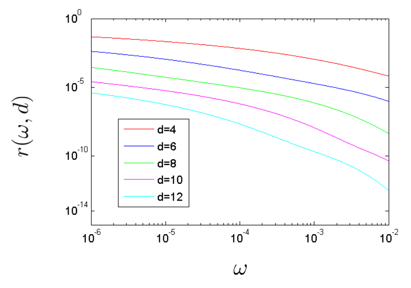
Next let us describe an explicit construction of the polynomials from Lemma 2. This material is based on Refs. [16, 32, 33]. Below we assume that . Define
We shall need Jacobi elliptic functions and . They are defined for by
where is the unique solution of
For each define
| (67) |
Define
Then
| (68) |
The coefficients can be easily computed using any computer algebra system such as MATLAB. We plot the worst-case relative error
| (69) |
as a function of for a few small values of on Fig. 1.
Finally, let us point out that can be approximated by a rational function of a given degree on the full interval . However, in this case the approximation error decays exponentially with . A simple example of such approximation has been proposed by Newman [35] (although Ref. [35] concerns with approximating the function, a simple change of variable shows that the same results hold for ). In contrast, Zolotarev’s approximation holds only on the interval but the approximation error decays exponentially with . Ref. [35] also demonstrates that rational approximations can be exponentially more accurate compared with the polynomial approximations of the same degree.
3.3 Approximation by low-rank Gaussian states
In this section we derive two corollaries of Theorem 2 that characterize ground states of quantum impurity models. Let be some ground state of the full Hamiltonian and be the covariance matrix of defined in Theorem 2. It is not hard to see that, roughly speaking, eigenvalues of are related to the number of bath excitations present in . For example, is the expected value of the number operator in the state . In the extreme case when the ground state itself is a Gaussian state (the ground state of ). More generally, the exponential decay stated in Theorem 2 is sufficient to show that is approximated by a relatively small number of Gaussian states. Furthermore, all excitations present in the bath can be “localized” on a small subset of modes by some Gaussian unitary operator. Recall that denotes the spectral gap of .
Corollary 1.
There exists a ground state of such that the following holds. For any there exists an integer
| (70) |
a Gaussian unitary operator , and some (non-Gaussian) state such that
| (71) |
Proof.
Let and be the state and corresponding matrix from Theorem 2. Let be a unitary operator such that
Define a new set of fermi modes such that . Then
| (72) |
Define a projector so that . Then and thus
where in the last inequality we used Theorem 2. Thus
for given by Eq. (70). Choose
where is the normalizing coefficient. The above shows that . Thus approximates within error . Finally, since projects onto a subspace in which the mode is empty, the state is the vacuum state for the subset of fermi modes . Therefore for some Gaussian unitary operator and some (non-Gaussian) state . ∎
From Eq. (71) one infers that is -close to a superposition of Gaussian states where is defined by Eq. (70). The next corollary states our best asymptotic upper bound on the number of Gaussian states one needs to approximate an exact ground state within a specified precision. This corollary provides a partial justification for the variational algorithm of Section 5 that minimizes the energy of over low-rank superpositions of Gaussian states. It also confirms our intuition (stated above) that eigenvalues of are related to the number of bath excitations in the ground state.
Corollary 2.
There exists a ground state of such that the following holds. For any there exists a normalized state such that and
| (73) |
where are orthonormal Gaussian states. Each state is an eigenvector of the particle number operator such that
| (74) |
Here is a universal constant. Furthermore, the projector
| (75) |
commutes with .
Proof.
We shall reuse some definitions and notation from the proof of Theorem 2 (repeated here for convenience). For any complex vector define a fermionic operator
Each canonical bath mode can be written as a linear combination of Majorana modes . Recall that the impurity is formed by the first modes . Define a linear subspace such that iff the expansion of in terms of the Majorana operators does not include .
As noted in Eqs. (30,29) we have for all and . Define to be the projector onto . Let and be as in Theorem 2. Write
for the eigenvalues of . By Cauchy’s interlacing theorem and Theorem 2 we have
where is the -th largest eigenvalue of . Let be an orthonormal basis of eigenvectors of , with
and . Define a new set of creation-annihilation operators such that
We have
| (76) |
Now divide up the set of positive integers into intervals of size . That is, let and define
Let . For each positive integer define
There are of these operators which are nonzero. Also note that Eq. (76) implies
| (77) |
for all . We have
| (78) |
where is another universal constant. Since the operators mutually commute, we can view as inducing a probability distribution given by
where is the projector onto Fock basis states with simultaneous eigenvalues for operators . Define
where is another universal constant. From Markov’s inequality and Eq. (78) we obtain
Applying a union bound we arrive at
Let us choose so that
| (79) |
i.e., . Then
Given a binary string let be the Fock basis vector with respect to the modes . In other words, for all . Define a projector onto a linear subspace
| (80) |
From the above we have . Defining we therefore have
Thus is -close to . We now show that projects onto a space of dimension upper bounded as
Fock basis states in the image of are indexed by bit strings of length where the last bits are unrestricted while the first bits are divided up into the intervals . The hamming weight of in interval is required to be at most when . Letting denote the number of bit strings of length with hamming weight at most we obtain
where in the second inequality we used the fact that . Recall that . Since for all we may bound
where is the binary entropy function. Therefore
| (81) |
Now using the inequality we get
Plugging this into Eq. (81) and using the fact that and gives
which completes the proof of Eq. (73). Here we take and to be the set of Fock basis states which span the image of , so that .
For future reference, let us summarize properties of that follow trivially from Corollary 2:
| (82) |
3.4 Energy distribution
Suppose is a ground state of the full Hamiltonian . In general, is not a ground state of the bath Hamiltonian . However, Corollary 2 of Theorem 2 implies that the average number of excitations in the bath is small as long as has a non-negligible spectral gap. Can we make a similar statement without any assumptions on the gap of ? In this section we prove a partial result along these lines that concerns the energy of excitations present in the bath. Namely, we show that any ground state of has most of its weight on a certain low-energy subspace of . Surprisingly, the energy cutoff that defines this low-energy subspace is independent of the strength of . The following theorem was inspired by an analogous theorem proved for quantum spin systems by Arad et al [19].
See 3
Proof.
Let us first establish some additional notation and conventions. Recall
where is given by Eq. (3) for some antisymmetric real matrix . We shall assume without loss of generality that has smallest eigenvalue equal to zero. Indeed, we may always add a constant times the identity to to ensure that this holds, and the statement of the theorem is identical before and after such a transformation. Without loss of generality we can also assume that
| (83) |
that is, the impurity modes are only coupled to the modes . Indeed, suppose is arbitrary. Let be the submatrix of formed by the first columns and the last rows. Choose an orthogonal matrix of size such that is an upper triangular matrix. Let . Then has zero matrix elements for and . Let be the Gaussian unitary operator such that , see Eq. (17). By definition, acts trivially on the impurity modes and the transformed bath Hamiltonian has a form Eq. (3) where satisfies Eq. (83).
We shall often work with a truncated version of the bath Hamiltonian defined as
| (84) |
where is a matrix obtained from by setting to zero the first rows and columns. By definition, acts trivially on the impurity modes and has ground energy zero.
Finally, define a Hamiltonian
From Eq. (83) one infers that acts non-trivially only on modes . Its norm is bounded as
| (85) |
where we used the triangle inequality, the fact that has rank at most , and .
The following lemma asserts that any ground state of the full Hamiltonian has most of its weight on a properly chosen low-energy subspace of that depends only on .
Lemma 3.
Let be the projector onto a subspace spanned by eigenvectors of with energy at most . Let be any ground state of . Then
| (86) |
Furthermore, for all one has
| (87) |
Here .
Proof.
Define a function
Then
| (88) |
Let be the ground energy of the full Hamiltonian. Note that since by assumption and . Computing the derivative of over one gets
By construction, commutes with , so that is hermitian. Furthermore, since we assumed that , one has . We arrive at
| (89) |
where
Let . Then
| (90) |
We claim that
| (91) |
for all . Indeed, since , it suffices to consider . By definition of one has
The fact that is quadratic in Majorana operators implies , where is a hermitian matrix of size (recall that and are anti-hermitian). Therefore
This implies
| (92) |
where in the second inequality we recalled that has rank at most .
From Eq. (92) we infer that and thus
| (93) |
Substituting this into Eq. (89) yields
| (94) |
Since is a ground energy of the full Hamiltonian, it is upper bounded by the energy of a tensor product of ground states of and . By assumption, and have zero ground energy, so
see Eq. (85), that is,
| (95) |
Since , one gets
| (96) |
Substituting this into Eq. (88) and choosing gives
| (97) |
which proves Eq. (86).
We proceed to proving Eq. (87). The first inequality in Eq. (87) simply states that the energy of a normalized state cannot be smaller than the ground energy of . Thus it suffices to prove the second inequality. Since commutes with and , one has
Using the above identity and the eigenvalue equation one gets
Recalling that , see Eq. (85) and using Eq. (86) leads to
Here we noted that for due to Eq. (86). ∎
We are now ready to complete the proof of Theorem 3. Let us first show that for all one has
| (98) |
Indeed, from and one gets
| (99) |
Let . Then
| (100) |
We may bound the first term in the righthand side of Eq. (100) as
| (101) |
Denote . Then Eq. (100) becomes
| (102) |
The same arguments as in the proof of Lemma 3 show that . Therefore
Since , this yields . Substituting this into Eq. (99) and choosing one gets Eq. (98).
4 Algorithms and complexity
In this section we consider the problem of approximating the ground energy of a quantum impurity model. We begin in Section 4.1 with some technical tools used in subsequent sections: a decoupling lemma which describes how to identify and decouple canonical bath modes which commute with the impurity, and a truncation lemma which shows that the ground energy can change by at most if we take all single-particle energies of below and round them up to . In Section 4.2 we present and analyze our quasipolynomial algorithm for approximating the ground energy of a quantum impurity model (that is, we prove Theorem 1). In Section 4.2 we consider the case where the full Hamiltonian has a constant spectral gap and in this case we give a polynomial time algorithm (proving Theorem 4). Finally, in Section 4.4 we present the proof of Theorem 5, that is, we show that the problem of estimating the ground energy of a quantum impurity model to inverse polynomial precision is contained in the complexity class QCMA.
4.1 Bath decoupling and truncation
In this Section we present two tools for simplifying quantum impurity problems.
The first tool is a decoupling lemma which is useful when the single-particle spectrum contains degeneracy. We say that a fermi mode is coupled to the impurity if . The decoupling lemma states that we may choose a set of fermi modes which diagonalize the bath Hamiltonian and such that at most of the modes with a given single-particle energy are coupled to the impurity.
Lemma 4 (Decoupling Lemma).
Let be a quantum impurity model, and write
| (106) |
where are the distinct single particle energies and contains all modes with energy . We may choose fermion operators such that is diagonalized as
| (107) |
where for all , and
| (108) |
A particle-number conserving Gaussian unitary such that for all can be computed in time.
Proof.
Suppose that the operators in Eq. (106) do not already satisfy the additional constraints in the Lemma. We will show how a Gaussian unitary transformation gives a new set of operators which satisfy these constraints.
Each operator can itself be expressed as a linear combination of the Majorana operators . For all we have
where is a complex matrix. A QR decomposition gives a unitary such that is in reduced row echelon form. We may compute using arithmetic operations. Setting
| (109) |
we see that the new creation and annihilation operators satisfy the fermion anticommutation relations and that
and therefore satisfies Eq. (106) with replaced by . From Eq. (109) we see that the Gaussian unitary which maps is associated with a linear transformation of fermion operators given by the block diagonal unitary . The total runtime for computing all blocks of this unitary is .
Now focus on a fixed , look at Eq. (109) and recall that is in reduced row echelon form. We see that there are at most modes in the set for which the right-hand side of Eq. (109) has a nonzero coefficient for the impurity Majorana modes . We partition where indexes these modes. Eq. (108) then follows, using the fact that acts non-trivially only on the modes and includes only even weight Majorana monomials. ∎
The second tool is a truncation lemma which bounds the change in the ground energy of when we truncate the single particle energies of the bath below a given threshold. Let a target precision be given and let index the single particle energies of which are at most , i.e.,
Define a truncated impurity model
| (110) |
Here we have set all energies to be equal to . Write for the ground energy of .
Lemma 5 (Truncation lemma).
Proof.
First define another Hamiltonian
and let its ground energy be . We have the operator inequality and thus . To prove the proposition we now show that . Let be a ground state of such that
It is always possible to choose such a ground state since all but of the modes in can be decoupled from the impurity. That is, lemma 4 implies that we may define new fermi modes such that
and for all and . This implies we may choose a ground state of such that for all and thus
Now
Therefore
∎
4.2 Quasipolynomial algorithm for general impurity models
In this Section we describe the quasipolynomial algorithm for approximating the ground energy and prove Theorem 1, restated here for convenience.
See 1
We begin by introducing some additional notation used in this section. Define an operator
which counts the number of excitations of the bath. For any define to be the subspace spanned by all eigenvectors of with eigenvalue at most . Corollary 2 states that (at least one) ground state of an impurity model is approximated to precision by a state in whenever
for some universal constant . In this section we are interested in approximating the ground energy rather than the ground state itself. We use corollary 2 and lemma 5 to prove the following lemma.
Lemma 6.
Let be a precision parameter. We have
| (111) |
whenever
| (112) |
where is a universal constant.
Proof.
The lower bound in Eq. (111) is trivial; below we prove the upper bound. Recall that we write for the spectral gap of the bath Hamiltonian , that is, all nonzero single-particle excitation energies are in the interval . Let be the desired precision.
As a first step we give a reduction to the special case where . The reduction is based on the truncation lemma (lemma 5). Let be given as in Eq. (110). By definition the bath Hamiltonian has spectral gap . We have the operator inequality and therefore
| (113) |
Suppose that lemma 6 holds for precision and Hamiltonian . Then, using lemma 5 and Eq. (113) we get
| (114) |
whenever
| (115) |
where is another universal constant. Eqs. (114,115) complete the reduction; they are Eqs. (111,112) for the original Hamiltonian , precision , and constant . Thus we have shown Lemma 6 follows from its special case where .
To complete the proof, we now establish the lemma assuming . Fix some and let be a normalized ground state of from Corollary 2. Let be the projector defined in Eq. (75). Corollary 2 states that , and that with , which implies . Using these facts we get
| (116) |
where in the last line we used . Now and, since both operators are diagonal over the same basis we also have . Using this fact and Eq. (82) we get
| (117) |
for some constant . In the last equality we substituted . Since and we have and therefore
| (118) |
where is another universal constant. Combining Eqs. (116,118) we get
| (119) |
Now we choose such that the right hand side is at most . It suffices to take
| (120) |
where is any universal constant satisfying . Indeed, with this choice we have
| (121) |
where we used the fact that the quantity in square parentheses is at most .
Thus
| (122) |
From Eqs. (82,118) we have and
where in the second inequality we used Eq. (121) and in the last inequality we used Eq. (120). This implies that the image of is contained in the subspace whenever
| (123) |
Thus, for all satisfying Eq. (123) we have
where in the second inequality we used Eq. (122). ∎
We now define a deformed impurity model. Let be a precision parameter, let be the smallest integer greater than or equal to the right hand side of Eq. (112) and consider a set of grid points
| (124) |
For each let be the smallest element of which is at least , so that
| (125) |
Define deformed Hamiltonians
Finally, define
| (126) |
The following lemma shows that is a good approximation to . Our algorithm for approximating is based on computing .
Lemma 7.
Proof.
Applying lemma 6 gives
Therefore
| (127) | ||||
| (128) |
where in the last line we used Weyl’s inequality. Here we use the notation to denote the restriction of an operator to a subspace . Now
and using Eq. (125) we arrive at
Thus
| (129) |
where in the last line we used the definition of . Plugging this into Eq. (128) completes the proof. ∎
Thus we have shown that to approximate it suffices to consider the deformed impurity model. Why is this useful to us? The total number of distinct single-particle energies is at most , which does not depend on . Since there are modes in total, we see that on average a single-particle energy of the deformed bath has degeneracy linear in . Because of this massive degeneracy, we may use the decoupling lemma to show that many of the degrees of freedom (modes) can be decoupled from the impurity.
Applying lemma 4 to the deformed impurity model we get fermion operators and subsets such that
| (130) |
such that and the modes in are decoupled from the impurity, that is,
| (131) |
For ease of notation, let us order the modes so that the decoupled ones appear first
Note that the total number of coupled modes is upper bounded by times the number of distinct single particle energy levels , that is,
| (132) |
For each define a Fock basis state with respect to the modes , i.e.,
| (133) |
Note that is an eigenstate of the operator with eigenvalue . Lemma 4 states that the decoupling transformation preserves particle number, that is,
| (134) |
By definition, the subspace is spanned by all eigenstates of the number operator Eq. (134) with eigenvalues at most . Therefore
Define a subspace
| (135) |
spanned by basis vectors where the decoupled modes are unoccupied. We now show that the minimization in Eq. (126) can be restricted to the subspace .
Lemma 8.
| (136) |
Proof.
Eqs. (130,131) imply for all and therefore
Thus the restriction is block diagonal in the basis with a block for each configuration of the decoupled modes. The smallest eigenvalue of is the smallest eigenvalue of one of the blocks. In particular, for some and we have
Now let and note that . Applying Lemma 4 we get
and therefore . Note that equality must hold since minimizes the energy of in . We have shown there exists with , which completes the proof. ∎
Let . We claim that the righthand side of Eq. (136) can be computed in time . Indeed Eq. (135) gives an orthonormal set of Gaussian states that spans . By construction, the deformed bath Hamiltonian is diagonal in this basis and one can compute a matrix element in time by summing up energies of all excitations present in . Thus one can compute the matrix of in the basis in time . Consider now the impurity Hamiltonian . By construction, is a linear combination of Majorana monomials . Using the generalized Wick’s theorem Eq. (27) one can compute a single matrix element in time . Thus one can compute the full matrix of in the basis in time . Once the matrices of and in the basis are computed, one can calculate using exact diagonalization in time . Recall that (to get rid of the factor of we may rescale the precision parameter without altering the asympotic runtime of the algorithm). This completes the proof of Theorem 1.
Remark: The above algorithm can be used to produce a low energy state of , the original (not deformed) impurity model. Indeed, in the last step of the algorithm, one may use an exact diagonalization routine which, along with the eigenvalue , computes a state satisfying . In this case we have
where we used Eq. (129). Combining this with the fact that , we see that the computed state satisfies
4.3 Efficient algorithm for gapped impurity models
Proof.
Let be the standard basis of . Let be the matrix defined in Eq. (3). Define a nested sequence of linear subspaces such that
for . We choose as the smallest integer such that . Obviously, . Let . By construction, is -invariant. Define a subspace
Let us agree that , so that . We get a direct sum decomposition
| (137) |
Note that is block-tridiagonal with respect to this decomposition, that is, whenever , , and . Indeed, assume wlog that . Then
whereas . Furthermore,
since is spanned by and .
Choose an orthonormal basis such that the first basis vectors span , the next basis vectors span and so on. The last basis vectors span . Define a new set of Majorana operators
| (138) |
Here is the -th component of . The operators obey the same commutation rules as . By construction, for and thus belongs to the algebra generated by . Transforming to the new basis we find that
| (139) |
where the two blocks have dimension and respectively. Moreover, is block-tridiagonal with non-zero matrix elements only between blocks , with . We conclude that
| (140) |
For simplicity, here we ignore the constant energy shift in Eq. (3). The terms and act on disjoint sets of modes and the ground energy of is the sum of their ground energies. Since is quadratic its ground energy is , which is easily computed from the singular value decomposition of . Thus we can concentrate on which acts on modes . Without loss of generality we shall assume is even in the following; if it is not even we may simply view as acting on modes in addition to one auxiliary Majorana mode. We can map to a Hamiltonian describing a 1D chain of qubits using the standard Jordan-Wigner transformation:
and
for . Here are the Pauli operators on the -th qubit. Since we have Majorana modes, the chain consists of qubits. We may coarse-grain the chain such that the first qubits form the first site, the next qubits form the second site, and so on (the last qudit may consist of qubits). Since is block tridiagonal with block size upper bounded as , we have
This block tridiagonal structure implies that after the Jordan-Wigner transformation the Hamiltonian describes a 1D chain of qudits with nearest-neighbor interactions. Each qudit has dimension at most
The chain has length . Since all of the above transformations are unitary, they preserve eigenvalues. Thus a gapped quantum impurity model can be efficiently mapped to a gapped 1D chain of qudits. One can approximate the ground state energy of the latter within error in time using MPS-based algorithms, see Ref. [20]. ∎
4.4 Containment in QCMA
We now consider the complexity of estimating the ground energy of a quantum impurity model to inverse polynomial precision. Formally, we consider the following decision problem (restated from Section 1.3). See Quantum impurity problem In this Section we prove the following theorem. See 5
We first review some facts concerning the representation of fermionic states on a quantum computer. Quantum states of fermionic modes are represented using qubits in the following way: for each , the Fock basis state is identified with the -qubit computational basis state . Majorana operators are represented via the Jordan-Wigner transformation:
| (141) | ||||
| (142) | ||||
| (143) | ||||
| (144) |
With this representation, a Gaussian state can be prepared efficiently on a quantum computer. A simple strategy to prepare any Gaussian state was given in Ref. [36]; we summarize it here for completeness.
Let a Gaussian state be specified up to a global phase by its covariance matrix , as defined in Eq. (18). For each and define a unitary
Using the Majorana commutation relations one can easily check that the state defined by
has covariance matrix
where is a “Givens rotation” which acts nontrivially only on the subspace spanned by basis vectors , and within this subspace its action is described by the matrix
Since is a real and antisymmetric matrix satisfying , there is an matrix such that , where is the covariance matrix of a standard basis state, see Eq. (19). The matrix can be computed efficiently using linear algebra, e.g., from the real Schur decomposition of [37]. It can then be decomposed as a product
for some angles and qubit indices , where . Such a decomposition can be computed, for example, using the strategy provided in Section 4.5.1 of the textbook Nielsen and Chuang [38] for decomposing a given unitary into two-level unitaries. We then have
for some global phase and computational basis state . From this expression it is evident that can be prepared efficiently, since the right hand side consists of unitaries , each of which is an exponential of a Pauli operator. In the following we will only need to use the slightly weaker statement that there exists a polynomial sized quantum circuit which prepares starting from .
We now give the proof of theorem 5.
Proof.
Let be given. Define and consider the truncated Hamiltonian from Eq. (110). Here where has spectral gap . The truncation lemma (lemma 5) states that
Therefore
Note . Also note that can be computed efficiently given ; we need only diagonalize the free fermion Hamiltonian which takes time . We have shown that the solution to the quantum impurity problem for with precision parameters is equivalent to the quantum impurity problem for with precision parameters . Below we give a QCMA protocol for the latter.
We use corollary 2 with (say) and Hamiltonian . Since , it implies that there exists a normalized state of the form
| (146) |
where are orthonormal Gaussian states, and where for some ground state of .
As discussed above, each Gaussian state can be prepared by a quantum circuit of size . This implies that there is also a polynomial sized quantum circuit which prepares with high probability (, say) and a flag qubit indicating success. Indeed, the unitary
can be implemented with a circuit of size (see for example Lemma 8 of Ref. [39]). Here the first register consists of ancilla qubits. Applying this unitary to the state one obtains . We may then perform the projective measurement , where
With probability we obtain the desired state . A quantum circuit which repeats this procedure times will produce with high probability.
Now we are ready to describe the QCMA protocol. The protocol begins with Merlin sending Arthur a classical description of a polynomial sized quantum circuit with an -qubit output register and a flag qubit. Ideally, Arthur would like this to be the circuit which prepares with probability (with the flag qubit indicating whether or not has been successfully prepared).
Arthur applies the given circuit to the all zeros input state and measures the flag qubit. If he obtains measurement outcome , then he performs the following test on the -qubit output register, otherwise he rejects. Using phase estimation [38] on , he measures the eigenvalue of within precision . The parameters of the phase estimation are chosen so that the probability of failure is at most (say). He accepts if the measured eigenvalue is at most .
Let us now analyze the completeness and soundness of this protocol. In the yes case Merlin can send the circuit which prepares with probability . In this case there is a ground state with energy such that , which implies . Thus, if the phase estimation succeeds, then with probability at least Arthur will measure an energy which is at most causing him to accept. Thus the total probability for Arthur to accept is the product of 0.99 (the probability that the flag qubit is measured to be ), 0.99 (the probability phase estimation succeeds), and (the probability that Arthur accepts given that phase estimation succeeds). We have shown that in the yes case Merlin can provide a classical witness which causes Arthur to accept with probability at least .
Next consider the no case. In this case the ground energy of is at least . Thus any eigenvalue of , when approximated within precision , is greater than Arthur’s threshold to accept, i.e., greater than . This means that, regardless of the circuit provided by Merlin, the only way Arthur will accept is if the phase estimation fails (which occurs with probability at most ). Thus, in the no case, Arthur rejects with probability at least .
Finally, note that Arthur’s computation has polynomial running time. He first performs the (polynomial-sized) circuit given to him by Merlin, and then performs phase estimation to precision and constant error probability. This phase estimation requires Arthur to implement Schrodinger time evolution for times . This can be done efficiently since is a sparse and efficiently row-computable Hamiltonian [40]. Indeed, since is a quantum impurity Hamiltonian it can be written as a sum of Majorana monomials, each of which corresponds to an -qubit Pauli.
∎
5 Simplified practical algorithm
In this section we describe a variational algorithm that minimizes the energy of a quantum impurity Hamiltonian over low-rank superpositions of Gaussian states. This algorithm provides an upper bound on the ground energy . We also describe an extended (less efficient) version of this algorithm that provides both upper and lower bounds on . We benchmark the method using the single impurity Anderson model [1].
Consider a system of fermi modes and a Hamiltonian composed of arbitrary quadratic and quartic Majorana monomials:
| (147) |
| (148) |
| (149) |
Here and are some real coefficients. We shall extend the range of all sums over Majorana modes to the interval assuming that unless . Since the Hamiltonian commutes with the parity operator , see Eq. (20), we can minimize the energy of in the even and the odd subspaces separately. Equivalently, one can minimize the energy of and within the even subspace. Since both minimizations are exactly the same, below we consider only the even subspace.
Our variational algorithm depends on an integer that we call a rank. Let
be a tuple of even Gaussian states with covariance matrices . The states may or may not be pairwise orthogonal. The algorithm works by minimizing an objective function defined as the smallest eigenvalue of restricted to the linear subspace spanned by states :
| (150) |
Here . Note that is uniquely determined by the covariance matrices .
We shall parameterize the covariance matrix of by a rotation such that
| (151) |
Here
is the covariance matrix of the vacuum state , see Eq. (19). Thus we have to minimize the objective function Eq. (150) over the group
where the direct product contains factors.
5.1 Rank- algorithm
Let us start from the simplest case , i.e. minimizing the energy of over all Gaussian states. This corresponds to a generalized Hartree-Fock method proposed recently by Kraus and Cirac [18] for simulation of interacting fermions on a lattice. Let . Applying Wick’s theorem Eq. (22) one gets
| (152) |
We initialize , where is chosen at random. The energy is then minimized by a greedy random walk algorithm. Each step of the walk generates a random rotation such that for some specified angle . A step is deemed successful if it decreases the value of the objective function, . In this case is replaced by . Otherwise remains unchanged. The angle is adjusted by keeping track of the fraction of successful steps . We fix some threshold value and adjust the angle as if and if . Here is a small constant. We empirically found that and works reasonably well.
5.2 Rank- algorithm
Define a Gram matrix such that . We can always choose the relative phase of and such that is a real matrix. Then
| (153) |
Here we used Eq. (23). Using the generalized Wick’s theorem Eq. (28) one gets
| (154) |
and
| (155) |
where
Using Eqs. (22,28) again one gets
| (156) |
| (157) |
Let and be hermitian operators with matrix elements
| (158) |
Here . Standard linear algebra implies that the objective function from Eq. (150) coincides with the minimum eigenvalue of a matrix
Equivalently, is the minimum eigenvalue of a generalized eigenvalue problem . Thus the above formulas allow one to compute in time . The most time consuming steps are clearly computing the inverse and the determinant of . We then minimize over using the same greedy random walk algorithm as in the rank- case. The only difference is that at each step we decide whether to rotate or at random.
5.3 Arbitrary rank
Suppose now that . Let be some fixed reference state used to compute inner products, see Section 2.4. We chose as a ground state of , but it could be an arbitrary Gaussian state. For each define
| (159) |
We can always choose the overall phase of such that are real and . Then Eq. (23) implies
| (160) |
where is the covariance matrix of the reference state. Define a Gram matrix with matrix elements , where . By normalization, one has . From Eq. (25) one gets
| (161) |
where
Note that and . Using the generalized Wick’s theorem Eq. (28) one gets
| (162) |
and
| (163) |
for all . Now we can compute by solving a generalized eigenvalue problem , where now and are hermitian operators defined by Eq. (158) and choosing the minimum eigenvalue .
We then minimize using the same greedy random walk algorithm as above. At each step of the walk we decide which matrix to rotate at random. After each rotation one has to compute the new coefficient and properly update matrices . This takes time .
5.4 SDP lower bound on the ground energy
Let be the exact ground energy of the full Hamiltonian . Clearly, the optimal value found by the variational rank- algorithm gives an upper bound on . Can we determine how good is this upper bound without computing exactly ? In this section we describe a simple extension of the rank- algorithm that gives both upper and lower bounds on . This enables us to benchmark the algorithm for large system sizes when exact diagonalization of is not feasible. We shall obtain a lower bound on using a semi-definite program (SDP) which is closely related to the 2-RDM method commonly used in the quantum chemistry [41].
Let be the set of all hermitian matrices of size . The SDP will depend on an integer and a list of operators acting on the Fock space . These operators must satisfy only two conditions. First, we require that the full Hamiltonian can be written as
| (164) |
for some coefficients . Second, we require that the identity operator on can be written as
| (165) |
for some coefficients . Define a space of linear dependencies
| (166) |
Clearly, is a linear subspace (over ). Let and fix a basis . Consider the following semi-definite program:
| (167) |
Here we view the coefficients and as matrix elements of hermitian matrices and .
Lemma 9.
For any normalized state there exists such that is a feasible solution of the SDP defined above and
| (168) |
Proof.
Choose such that for all . A direct inspection shows that obeys all constraints of the SDP and Eq. (168) holds. ∎
The lemma implies that the optimal value of the SDP provides a lower bound on the ground energy . One can easily check that this lower bound is tight for free fermion Hamiltonians defined in Eq. (3) if one chooses and for . Here are the Majorana operators defined in Eq. (1). Furthermore, one can easily check that the lower bound is tight for an arbitrary Hamiltonian if one chooses and the list of operators includes all Majorana monomials with . Our choice of the operators for quantum impurity models will be a mixture of these two extreme cases.
Let be the optimal solution of the program Eq. (167). Standard duality arguments show that whenever
| (169) |
for some . Here and are Lagrangian multipliers for the constraints and . Thus any feasible solution of Eq. (169) gives a lower bound on the ground energy, namely, .
Consider an impurity model such that acts on the modes . How do we choose and the operators to define the above SDP ? Let be the exact ground state of . By Corollary 1, one can localize all bath excitations present in on a small subset of modes by some Gaussian unitary , that is,
| (170) |
Here is a small precision parameter and is determined by Eqs. (70). Suppose first that we can guess the integer and the Gaussian unitary operator that achieve the desired approximation precision . Empirically, we found that the following choice of the operators achieves a very good lower bound on at a reasonable computational cost. First, define an extended list of Majorana operators such that
| (171) |
and
| (172) |
Note that the state in Eq. (170) can be obtained from the vacuum by some combination of the operators . Let us choose
| (173) |
and choose the operators as
| (174) |
Here denotes the product of all operators with . One can easily check that the list Eq. (174) satisfies condition Eq. (164) for any impurity Hamiltonian with quartic interactions acting on the first modes . It is also clear that this list satisfies condition Eq. (165) since, for example, .
In practice, we can obtain a good guess of and in Eq. (170) by examining the optimal variational state found by the rank- algorithm. Namely, consider the covariance matrix
Using the generalized Wick’s theorem Eq. (28) one can compute in time since is specified as a superposition of Gaussian states. Let eigenvalues of be , where
are singular values of . If were the exact ground state, Theorem 2 implies66 6 In this paper we use two versions of a covariance matrix – one for Majorana operators, see Eq. (18), and the other for creation-annihilation operators, see Eq. (4). If the latter has eigenvalues then the former has eigenvalues , where . that the singular values rapidly approach one as increases. We found empirically that this is also true for the optimal variational state . Let be the smallest integer such that for all , where is some fixed precision parameter. In our simulations we choose . One can always transform into a block-diagonal form such that
for some . Let be the Gaussian unitary that implements the rotation , see Eq. (17). Then
that is, all bath excitations present in the state are ”localized” on the first modes and we can write for some -mode state .
We define the SDP according to Eqs. (171,172,173,174), where is the Gaussian unitary constructed above. This defines the SDP lower bound on the ground energy for a given variational state and a precision parameter .
To benchmark the variational algorithm and the SDP method we chose the single impurity Anderson model [1]. This model has a Hamiltonian , where
for some . This corresponds to the impurity of size (we note that is the smallest impurity size that gives rise to a non-trivial impurity model since any even Hamiltonian acting on Majorana modes must be quadratic). For simplicity, we chose as the critical Majorana chain [28] with periodic boundary conditions:
It is well-known [42, 43] that has a unique ground state with parity and the spectral gap proportional to .
Let be the ground energy of . For each choice of and we numerically computed two numbers and such that
The upper bound is the minimum energy found by the rank- variational algorithm. In our simulations we only used and . The lower bound was computed using a combination of the rank- variational algorithm and the SDP method with as described above. The corresponding SDP has size , see Eq. (173,174). Figure 2 shows the gap as a function of the system size for several values of . In all cases the rank- algorithm approximates the ground energy within an additive error less than and we were able to estimate within the first eight significant digits, see Eq. (175).

|
|
(175) |
References
- [1] P. W. Anderson. Localized magnetic states in metals. Phys. Rev., 124:41–53, 1961.
- [2] Jun Kondo. Resistance minimum in dilute magnetic alloys. Progress of Theoretical Physics, 32(1):37–49, 1964.
- [3] Kenneth G Wilson. The renormalization group: Critical phenomena and the Kondo problem. Reviews of Modern Physics, 47(4):773, 1975.
- [4] L. Kouwenhoven and L. Glazman. Revival of the Kondo effect. Physics World, 14(1):33, 2001.
- [5] W.J. De Haas and G.J Van Den Berg. The electrical resistance of gold and silver at low temperatures. Physica, 3(6):440–449, 1936.
- [6] Antoine Georges. Strongly correlated electron materials: Dynamical mean field theory and electronic structure. AIP Conference Proceedings, 715(1):3–74, 2004.
- [7] G. Kotliar, S. Savrasov, K. Haule, V. Oudovenko, O. Parcollet, and C. Marianetti. Electronic structure calculations with dynamical mean-field theory. Reviews of Modern Physics, 78(3):865, 2006.
- [8] B. Bauer, D. Wecker, A. J. Millis, M. B. Hastings, and M. Troyer. Hybrid quantum-classical approach to correlated materials, 2015. arXiv:1510.03859.
- [9] J. M Kreula, L. García-Álvarez, L. Lamata, S. R Clark, E. Solano, and D. Jaksch. Few-qubit quantum-classical simulation of strongly correlated lattice fermions. arXiv:1606.04839, 2016.
- [10] S. Gharibian, Y. Huang, Z. Landau, and S. W. Shin. Quantum Hamiltonian complexity. Found. Trends Theor. Comput. Sci., 10(3):159–282, 2015.
- [11] A. Yu. Kitaev, A. H. Shen, and M. N. Vyalyi. Classical and Quantum Computation. American Mathematical Society, Boston, MA, USA, 2002.
- [12] N. Schuch and F. Verstraete. Computational complexity of interacting electrons and fundamental limitations of density functional theory. Nature Physics, 5(10):732–735, 2009.
- [13] D. Bini and V. Y. Pan. Computing matrix eigenvalues and polynomial zeros where the output is real. SIAM Journal on Computing, 27(4):1099–1115, 1998.
- [14] P.B. Wiegmann and A.M. Tsvelick. Exact solution of the Anderson model: I. J. of Physics C: Solid State Physics, 16(12):2281, 1983.
- [15] N. Kawakami and A. Okiji. Exact expression of the ground-state energy for the symmetric Anderson model. Phys. Lett. A, 86(9):483–486, 1981.
- [16] E. Zolotarev. Application of elliptic functions to questions of functions deviating least and most from zero. Zap. Imp. Akad. Nauk. St. Petersburg, 30(5):1–59, 1877.
- [17] D. J. Brod and A. M. Childs. The computational power of matchgates and the XY interaction on arbitrary graphs. Quant. Inf. & Comp., 14(11-12):901–916, 2014.
- [18] C. Kraus and J.I. Cirac. Generalized Hartree-Fock theory for interacting fermions in lattices: numerical methods. New J. of Phys., 12(11):113004, 2010.
- [19] I. Arad, T. Kuwahara, and Z. Landau. Connecting global and local energy distributions in quantum spin models on a lattice. Journal of Statistical Mechanics: Theory and Experiment, 3:033301, March 2016. arXiv:1406.3898.
- [20] Z. Landau, U. Vazirani, and T. Vidick. A polynomial time algorithm for the ground state of one-dimensional gapped local Hamiltonians. Nature Physics, 11(7):566–569, 2015.
- [21] D. Aharonov and T. Naveh. Quantum NP - A Survey. arXiv:quant-ph/0210077, 2002.
- [22] S. Bravyi and D. Gosset. Improved classical simulation of quantum circuits dominated by clifford gates. Phys. Rev. Lett., 116:250501, Jun 2016.
- [23] B. M. Terhal and D. P. DiVincenzo. Classical simulation of noninteracting-fermion quantum circuits. Phys. Rev. A, 65(3):032325, 2002.
- [24] S. Bravyi. Lagrangian representation for fermionic linear optics. Quant. Inf. and Comp., 5(3):216–238, 2005.
- [25] M. Wimmer. Efficient numerical computation of the Pfaffian for dense and banded skew-symmetric matrices. arXiv:1102.3440, 2011.
- [26] J. Rubow and U. Wolff. A factorization algorithm to compute Pfaffians. Computer Physics Communications, 182(12):2530–2532, 2011.
- [27] J. Schliemann, J. I. Cirac, M. Kuś, M. Lewenstein, and D. Loss. Quantum correlations in two-fermion systems. Physical Review A, 64(2):022303, 2001.
- [28] A. Yu. Kitaev. Unpaired Majorana fermions in quantum wires. Physics-Uspekhi, 44(10S):131, 2001.
- [29] Per-Olov Löwdin. Quantum theory of many-particle systems I. Physical Review, 97(6):1474, 1955.
- [30] A. Kennedy. Approximation theory for matrices. Nuclear Physics B-Proceedings Supplements, 128:107–116, 2004.
- [31] T.-W. Chiu, T.-H. Hsieh, C.-H. Huang, and T.-R. Huang. Note on the Zolotarev optimal rational approximation for the overlap Dirac operator. Phys. Rev. D, 66(11):114502, 2002.
- [32] A.A. Gončar. Zolotarev problems connected with rational functions. Sbornik: Mathematics, 7(4):623–635, 1969.
- [33] Y. Nakatsukasa and R. W. Freund. Computing fundamental matrix decompositions accurately via the matrix sign function in two iterations: The power of Zolotarev’s functions. http://eprints.ma.man.ac.uk/2414/01/papersirevrevrevf_tosiam.pdf, 2015.
- [34] G. D. Anderson, M. K. Vamanamurthy, and M. Vuorinen. Functional inequalities for complete elliptic integrals and their ratios. SIAM Journal on Mathematical Analysis, 21(2):536–549, 1990.
- [35] D.J. Newman. Rational approximation to . The Michigan Mathematical Journal, 11(1):11–14, 1964.
- [36] D. Wecker, M. B. Hastings, N. Wiebe, B. K. Clark, C. Nayak, and M. Troyer. Solving strongly correlated electron models on a quantum computer. Phys. Rev. A, 92(6):062318, 2015.
- [37] G.H. Golub and C.F. Van Loan. Matrix Computations. Johns Hopkins Studies in the Mathematical Sciences. Johns Hopkins University Press, 1996.
- [38] M.A. Nielsen and I.L. Chuang. Quantum Computation and Quantum Information. Cambridge Series on Information and the Natural Sciences. Cambridge University Press, 2000.
- [39] A. M. Childs, R. Kothari, and R. D. Somma. Quantum linear systems algorithm with exponentially improved dependence on precision. arXiv:1511.02306, 2015.
- [40] D. Aharonov and A. Ta-Shma. Adiabatic quantum state generation and statistical zero knowledge. In Proceedings of the Thirty-fifth Annual ACM Symposium on Theory of Computing, STOC ’03, pages 20–29, New York, NY, USA, 2003. ACM.
- [41] D. A. Mazziotti. Variational two-electron reduced density matrix theory for many-electron atoms and molecules: Implementation of the spin-and symmetry-adapted T2 condition through first-order semidefinite programming. Phys. Rev. A, 72(3):032510, 2005.
- [42] T. D. Schultz, D. C. Mattis, and E.H. Lieb. Two-dimensional Ising model as a soluble problem of many fermions. Reviews of Modern Physics, 36(3):856, 1964.
- [43] Pierre Pfeuty. The one-dimensional Ising model with a transverse field. Annals of Physics, 57(1):79–90, 1970.
- [44] Philippe Francesco, Pierre Mathieu, and David Sénéchal. Conformal field theory. Springer Science & Business Media, 2012.
- [45] R. Cleve, D. Leung, L. Liu, and C. Wang. Near-linear constructions of exact unitary 2-designs. arXiv:1501.04592, 2015.
- [46] Thomas Koshy. Catalan Numbers with Applications. Oxford University Press, USA, 2008.
Appendix A Proof of the inner product formulas
In this appendix we prove the inner product formulas and the generalized Wick’s theorem of Section 2.4. Let be an arbitrary operator acting on the Fock space . Expanding in the basis of Majorana monomials , , one gets
for some coefficients . Here and in the rest of this section all sums over binary strings have range . An operator as above can be described by a generating function
where are formal variables obeying commutation rules of the Grassmann algebra, that is,
An integral over Grassmann variables is a linear functional defined by
The action of extends by linearity to an arbitrary function by expanding in the basis of Grassmann monomials . More details on the formalism of Grassmann variables can be found in [44, 24]. Let be an anti-symmetric matrix of size . We shall consider as a column vector and write for the corresponding row vector. Then
Suppose is a Gaussian state with a covariance matrix and let . Wick’s theorem Eq. (22) can be rephrased as
| (176) |
We shall need the following well-known formulas for Gaussian integrals:
| (177) |
| (178) |
Here is another vector of Grassmann variables.
Now we can easily prove Eq. (23). Define a bilinear form
Here . Then if and if . Furthermore,
if and the integral is zero if . Here both and are vectors of Grassmann variables and . Let , be arbitrary operators on and , be their generating functions. The above shows that
| (179) |
Suppose now that are projectors onto some pure Gaussian states with covariance matrices and parity . Substituting Eq. (176) into Eq. (179), taking the integral over using Eq. (178) and taking the integral over using Eq. (177) one gets
Here we noted that .
Next let us prove Eq. (24). Consider any even-weight strings such that
| (180) |
Here and below addition of binary strings is performed modulo two. Let be the total parity operator defined in Eq. (20). A simple algebra shows that
| (181) |
Furthermore, the trace is zero whenever .
Suppose are vectors of Grassmann variables. Let . A simple algebra shows that
| (182) |
Furthermore, the integral is zero whenever .
We shall say that an operator acting on is even if its expansion in the basis of Majorana monomials includes only even-weight monomials. Let be any even operators on and , , be their generating functions. Comparing Eqs. (181,182) one concludes that
| (183) |
Suppose now that are projectors onto some pure Gaussian states with covariance matrices respectively. Recall that any Gaussian state has a fixed parity, that is, for some . Clearly unless all states have the same parity: . Using Eqs. (176,177) one gets
This is equivalent to Eq. (24). To prove Eq. (25) let us come back to Eq. (183) and take a partial integral over . Applying Eq. (178) and noting that one gets
Next let us take a partial integral over . Applying Eq. (178) one gets
where
Taking into account that one can rewrite as
Finally, taking the integral over using Eq. (177) yields
This is equivalent to Eq. (25) since .
Next let us prove the generalized Wick’s theorem Eq. (27). Choose a Gaussian unitary such that , where is the Hamming weight of . Let be the corresponding rotation defined by Eq. (17). Replacing each state by is equivalent to replacing the covariance matrix by . Thus suffices to prove Eq. (27) for the special case .
Define . We would like to compute the generating function describing . Using the standard Wick’s theorem Eq. (22) one gets
Here we noted that and . Therefore
It follows that has a generating function
Here is a vector of Grassmann variables. Let us construct a linear map acting on Grassmann monomials such that
for all . This would imply that
It will be convenient to represent , where has length and has length . Then simple algebra shows that
| (184) |
Here is a vector of Grassmann variables. Let and be the generating functions of projectors onto and . Applying Eq. (183) and using the new definition of one arrives at
| (185) |
and
| (186) |
Combining Eqs. (184,186) one arrives at
Evaluating the integral using Eq. (177) gives
| (187) |
where is a matrix of size such that if is the position of the -th nonzero of and otherwise. Furthermore, is a diagonal matrix of size such that . Combining this and Eq. (185) proves the generalized Wick’s theorem Eq. (27).
Appendix B Fast norm estimation
Here we describe an algorithm for estimating the norm of a state represented as a superposition of Gaussian states. It is a Gaussian version of an algorithm presented in Ref. [22] for superpositions of stabilizer states. Suppose our goal is to compute the norm of a state
where and are normalized Gaussian states. The states are not assumed to be orthogonal. We assume that we are explicitly given the coefficients and that each Gaussian state is specified by its covariance matrix and its inner product with a reference Gaussian state .
A naive classical algorithm for computing is to expand
and then to compute each term in the sum using the inner product algorithm from Section 2.4. The runtime of this naive algorithm scales quadratically with . Below we present a Monte Carlo algorithm which estimates with runtime scaling only linearly with . In particular, we prove the following lemma. In the lemma it is assumed that the state is classically represented as described above.
Lemma 10.
Let where are Gaussian states and . There is a classical algorithm which takes as input a precision parameter , a failure probability , and the state and outputs an estimate such that, with probabilty at least we have
The runtime of the algorithm is .
In the remainder of this Appendix we prove the lemma. As noted above, this result is a Gaussian analog of a similar norm estimation algorithm given in Ref. [22] for superpositions of stabilizer states. However, while that algorithm uses the fact that stabilizer states form a -design, one can show that, strictly speaking, no ensemble of Gaussian states has this property. To prove lemma 10 we follow a technique from Ref. [45] which established a criterion called Pauli mixing for an ensemble of Clifford unitaries to form a -design. We define an analogous criterion which we call Majorana mixing for ensembles of Gaussian unitaries and we show how to use this criterion (rather than the -design property) in the norm estimation algorithm.
B.1 Symmetric tensor products of Gaussian states
Recall that the Majorana monomials
form a basis (over ) for the space of Hermitian operators acting on the Hilbert space of fermi modes. For any state we denote for the coefficients of its expansion
| (188) |
Define an operator
which acts on , and write for its null space. To construct a basis for first note that the commuting operators can be simultaneously diagonalized. We define a complete orthonormal basis of , where
A subset of these basis vectors span
| (189) |
and the projector onto is
| (190) |
We now derive a set of constraints on the coefficients of a state .
Proposition 2.
There exist real numbers such that
for all with .
Proof.
We are interested in the subspace because it contains any symmetric tensor product of fermionic Gaussian states.
Proposition 3.
Let where is a fermionic Gaussian state. Then .
Proof.
First consider the special case in which is a standard basis state. Here . In this case follows directly from
For general Gaussian , let be a Gaussian unitary and such that . Then for some , and
Therefore
∎
B.2 Ensembles of Gaussian unitaries and Majorana mixing
In this section we consider probability distributions over Gaussian unitaries and we define a notion of Majorana mixing for such ensembles. We then show that a certain channel derived from any Majorana mixing ensemble satisfies
The definitions and proof strategy are based on reference [45] where a similar notion of Pauli mixing is shown to be sufficient for an ensemble of Clifford unitaries to form a unitary -design.
For each define
Definition 1.
A probability distribution over Gaussian unitaries is said to be Majorana mixing if
for all .
Let us now present a simple example of an ensemble which is Majorana mixing. To begin we define an ensemble of matrices. To choose a matrix from this ensemble we simply select a uniformly random permutation and let be the corresponding permutation matrix. Next define where is a Gaussian unitary such that . To see that is Majorana mixing, note that
Here the permutation associated to permutes the bits of . In our ensemble the permutation is uniformly random and therefore is mapped to where is uniformly random among bit strings with the same Hamming weight as . This shows that is Majorana mixing.
For any distribution we define a channel which consists of first applying a uniformly random symmetric Majorana monomial and then applying where is a random Gaussian unitary drawn from . In other words
| (193) |
Lemma 11.
Let with and let be an ensemble of Gaussian unitaries which is Majorana mixing. Then
| (194) |
Proof.
The proof is based on Appendix D of [45]. We use the expansion (188) and linearity of . We first show that whenever . Note that since we have or . Without loss of generality suppose . We shall use the following fact
Proposition 4.
For all with and there exists such that and .
Proof.
The Majorana monomials satisfy
The desired bit-string is therefore a solution to linear equations in variables over , namely and . Equivalently,
where and . To show there exists a solution for we must show that the vectors defined by and satisfy and . Note follows from our assumption that . Since we have whenever . On the other hand if then by definition we have
which shows . ∎
So let satisfy and . Then
Next consider . Since
for all we get
where in the last equality we used the fact that is Majorana mixing. Using linearity we arrive at
| (195) |
where are the coefficients defined in Proposition 2. It remains to show that the right-hand sides of Eqs. (195,194) are equal up to normalization. Inspecting Eq. (190) we see that monomials with do not appear and that monomials corresponding to a given Hamming weight appear with equal weight, i.e.,
| (196) |
where are some coefficients. Finally, applying Proposition 2 to the density matrix forces , which completes the proof. ∎
B.3 Estimating the norm of a superposition of Gaussian states
Let
where are Gaussian states. Define a random variable
| (197) |
Here is a random Gaussian state of the form
| (198) |
where is chosen uniformly at random and is a random Gaussian unitary chosen from a Majorana mixing ensemble . For concreteness in the following we will assume it is taken from the ensemble defined in the previous section. Since Eq. (197) is insensitive to the global phase of , we obtain the same random variable by choosing
| (199) |
where is chosen uniformly at random and is a random Gaussian unitary chosen from .
The expected value of is
We now use the results of the previous section to upper bound the variance of .
Lemma 12.
.
Proof.
Now consider an estimator
where each is an independently chosen random state of the form Eq. (198). Then has expected value and variance
Applying Chebyshev’s inequality we obtain
Choosing
| (200) |
ensures that with probability at least we have
Finally, let us describe the algorithm which computes .
The first step is to choose the random Gaussian states . To choose each Gaussian state we select a random bit string and a random Gaussian unitary from the ensemble . Recall from the previous section that is chosen by selecting a uniformly random permutation matrix . Letting be the covariance matrix of the basis state , the covariance matrix of is which can be computed in time .
The second step is to compute for each . We have
where each term of the sum can be computed in time using the inner product formula from Section 2.4. This step therefore requires time for each . Computing from this data is then straightforward.
The total runtime to compute using this algorithm is