The double-layer structure of overscreened surfaces by smeared-out ions
Abstract
The present work focuses on the structure of a double-layer of overscreened charged surfaces by smeared-out charges and probes the link between the structure of a double-layer and the bulk properties of an electrolyte with special view to the role of the Kirkwood crossover. Just as the Kirkwood line divides a bulk solution into a fluid with monotonic and oscillatory decaying correlations, it similarly separates charge inversion into two broad domains, with and without oscillating charge density profile. As initially oscillations may appear like a far-field occurrence, eventually they develop into a full fledged layering of a charge density.
I Introduction
In our previous work we reported the possibility of charge inversion for ions with charge distribution [1, 2] (the so called smeared-out ions). Because the phenomenon was captured within the mean-field model, correlations have no role in this behavior. Rather the explanation lies in reduced interactions at short separations due to elimination of a divergence in the Coulomb functional form, which permit more compact structure of counterions. This is in contrast to point charges, , where charge inversion occurs when strong correlations give rise to lateral ordering of counterions within a double-layer. Such a correlation-based mechanism can only arise within an improved theory beyond the mean-field [3, 4, 5, 6].
In Refs. [1, 2] we laid primary stress on the fact that a charge density profile (and an electrostatic potential) changes sign as a function of distance from a charged surface and gave less attention to the far-field region, especially the presence in that region of oscillations. Our interest in the far-field region was recently revived by a demonstration in Ref. [7] of the existence of the Kirkwood crossover – a point where a charge-charge correlation function changes from a monotonically to an oscillatorily decaying profile – and a possible connection to our own results in Ref. [1]. As oscillations in charge density profile around zero imply charge inversion (or rather an entire sequence of inversions), we began to wonder about a possible role of the Kirkwood crossover in the mechanism of charge inversion. If indeed charge inversion is coextensive with the onset of oscillatory decay, one may conclude that inversion is triggered by the Kirkwood crossover, and, therefore, is completely determined by the properties of a bulk electrolyte and independent of a charged surface. If, however, there exists a possibility of charge inversion for monotonically decaying profile, then the picture is more subtle.
The aim of the present work is to investigate charge inversion of smeared-out ions with special attention to the far-field region and the connection with the Kirkwood crossover. Before proceeding, however, we review some basic ideas that will sketch a larger context and help to understand our motivations and perplexities about the far-field region.
A characteristic of a fluid is a short-range translational order whereby correlations of a fluctuating variable decay exponentially as , where implies the correlation length and is some algebraic function. Now, if we turn to an inhomogeneous fluid, we find that a density perturbation falls off exponentially as it merges with a uniform fluid, , with the same exponential decay as that for correlations. ( depends on the geometry of a perturbation). This universality of an exponential decay is a consequence of the linear response theory wherein a perturbation is expressed as a superposition of fluctuations. Nonlinear effects of a larger perturbation do not invalidate this interpretation as in the region where a perturbation merges with a bulk fluid a perturbation is again small and the linear regime recovered.
A picture becomes more interesting if one considers dense fluids where the short-range translational order attains some degree of organization and the profile of a density-density correlation function develops a regular oscillating structure, albeit, that still decays exponentially. There are now two parameters describing a decay of correlations: a correlation lenght and a wavelength . The point where oscillations first appear is known as the Fisher-Widom crossover [8, 9]. It is a crossover in a sense that it does not entail any macroscopic changes nor generate discontinuities in thermodynamic quantities. Discontinuous behavior, however, is observed in the scaling of the correlation length : before the Fisher-Widom line decreases as a function of increasing density, after the crossover the trend changes and increases with a denser fluid. Now, if we turn to inhomogeneous fluids, we find a similar structure in a density decay: an exponentially decaying oscillatory profile.
An analogous picture emerges for electrolytes, except now the relevant quantities are a charge density and a charge-charge correlation function. Here we also encounter a crossover from a monotonic to oscillatory decay that goes by the name of the Kirkwood crossover [10, 11, 12]. An interesting consequence of having oscillations in a charge density around zero is a repetitive charge inversion. This type of charge inversion depends only on the conditions of a bulk that control the quantities and and cannot be induced by a surface charge or any specific feature of a perturbation.
On the other hand, we have a more ”conventional” mechanism for charge inversion, wherein charge inversion is regarded as an effect of a renormalized effective charge and does not assume any change in the far-field decay, which remains monotonic. (The idea of an ”effective charge” entails the idea of a ”dressed surface”, a surface comprised of a bare surface charge plus an adjacent layer of counterions that together reduce an absolute value of a bare charge). As the present work is entirely devoted to the mean-field analysis, any renormalization of an effective charge comes from nonlinear contributions of the mean-field theory, wherein the scaling of an effective charge corresponds to the scaling of a magnitude of a monotonically decaying profile. Such nonlinear renormalization of an effective charge carried out for point-ions does not lead to charge inversion but merely to charge saturation. To capture charge inversion for point-ions one needs to go beyond the mean-field level of description [3, 4, 5, 2].
This work is organized as follows. In section II we formulate the mean-field theory for smeared-out ions. In section III we carry out the linear analysis to obtain the screening parameters and the location of the Kirkwood crossover for Gaussian distributed charges. In section IV we consider the full mean-field theory and focus on the renormalization of an effective surface charge for monotonically decaying profiles (prior to the Kirkwood crossover) and mark the region where charge inversion due to renormalization becomes possible. In section V we make connection to a related system of dumbbell ions. Finally, in section VI we conclude the work.
II The mean-field description
Within the standard representation, an electrolyte is made up of different species of point-charges, and the Poisson equation is given by
| (1) |
where is the electrostatic potential, and is a number density and a charge of a species , respectively, and is the dielectric constant of a solvent medium. If we move away from a point-charge description and consider ions represented as smeared-out charges within a spherically symmetrical distribution and normalized as , then the Poisson equation is
| (2) |
and the case recovers the Poisson equation for point charges. Note that since an ion has an extension, it does not need to be at to contribute to a charge density at . Contributions come from a distribution centered at , leading to a nonlocal term.
The mean-field expression for a number density of smeared-out ions is
| (3) |
where in is the bulk concentration of a species , and . The nonlocality reflects the idea of an entire ion interacting with an electrostatic potential .
Inserting the mean-field number density into the Poisson equation of Eq. (2) yields a modified Poisson-Boltzmann equation for smeared-out ions,
| (4) |
Not surprisingly, correlational contributions diminish with increasing size of an ion. Consequently, the mean-field theory becomes virtually an exact model for representing ions with broad charge distributions. Our interest lies specifically in such a mean-field regime, where correlational contributions are minimal, so that any deviations from the point-charge model can be exclusively attributed to finite size.
III Linear analysis
As mentioned in the introduction, to determine an asymptotic region within any theory (here we have in mind screening parameters or a correlation length) the linear analysis is sufficient. Nonlinear contributions of the full mean-field model do not modify these parameters, while the linearized version of any theory is simpler and easier to handle.
Keeping only the linear terms of the modified PB equation in Eq. (4) we get
| (5) |
For a symmetric monovalent electrolyte, where the net charge of an ion is ( is the fundamental charge), the distributions are , and is the salt concentration in a bulk, the above equation further simplifies as
| (6) |
We perturb the uniform system by fixing a single ion at the origin, then obtain an electrostatic potential from the linear theory,
| (7) | |||||
Note that a fixed particle is taken to be positive. Fourier transforming the above equation yields
| (8) |
and the potential in the Fourier space is
| (9) |
At this point we introduce more convenient reduced units,
| (10) |
where , is the Bjerrum length, and is the Debye screening parameter. The electrostatic potential in real space is then obtained from inverse Fourier transform,
| (11) |
For the case of point charges and the above integral evaluates to a familiar screened potential .
For particles with an arbitrary distribution , the integral in Eq. (11) can be conveniently handled using the residue theorem. To adopt the method to the present problem, we alter the limits of the integration as
| (12) |
which is allowed as long as is an even function, in which case the imaginary part cancels out. The need to alter the integration limits will become clear as we outline the details of the method.
In complex analysis the value of an integral along a closed curve can be expressed as a sum of residues inside the region enclosed by ,
| (13) |
In this case is a complex variable, and is a residue of at a pole . A value of a residue corresponds to a coefficient in the expansion
| (14) |
carried out in the neighborhood of a pole . A pole is said to be simple if .
In order to use Eq. (13) to evaluated the integral in Eq. (12), the curve should incorporate the real axis, while the integral along the remaining curve (let’s say a half circle with radius ) should evaluate to zero. If satisfied, then a potential can be represented as
| (15) |
with the integrand given by
| (16) |
Poles, being singularities of the complex plane, correspond to zeros of the denominator of ,
| (17) |
If poles enclosed by are simple, and by representing as a quotient of two functions , the residues are given by
| (18) |
Together with Eq. (12) and Eq. (13), an electrostatic potential is then given by
| (19) |
It is now clear that the poles, expressed as,
| (20) |
characterize a screening parameter and a wavenumber of each term in Eq. (19). Since the linear theory accurately describes only a far-field region, we are only interested in the dominant term, that is, the pole with the smallest .
Note that only a strictly imaginary yields a monotonically decaying function. On the other hand, a strictly real yields a solid like structure with a long-range translational order. A fully complex pole determines an oscillating exponentially decaying profile.
III.1 as a Gaussian distributed function
As a specific case, we consider ions with a Gaussian distributed charge,
| (21) |
whose Fourier transform is
| (22) |
and an electrostatic potential within a linearized mean-field theory is given by
| (23) |
The poles satisfy
| (24) |
or, after rearrangement,
| (25) |
where appears as a function of . But being interested in as a function of , we look for an inverted relation that, in fact, is provided by the Lambert multivalued function [13, 14]
| (26) |
where denotes a particular branch, with being the principal branch. The Lambert function is the inverse relation of the function . It turns out that this function is quite ubiquitous in nature. For example, it provides an exact solution to the quantum-mechanical double-well Dirac delta function model for equal charges [13].
The poles are now expressed as
| (27) |
and the electrostatic potential within the linear mean-field theory is
| (28) |
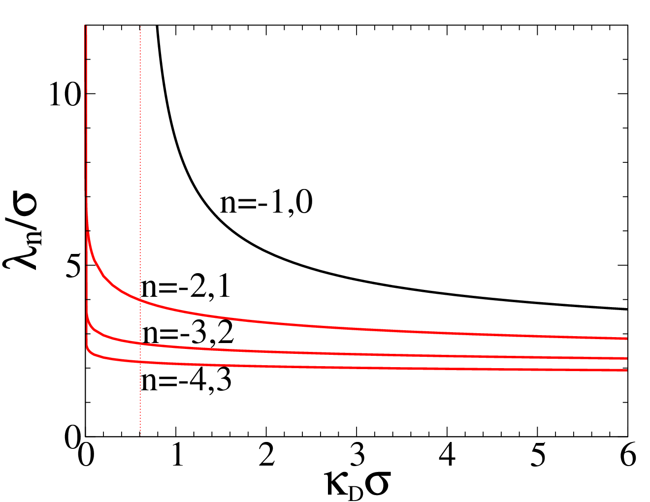
In Fig. (1) we plot the screening parameters , obtained from poles, , and given by
| (29) |
for a number of initial branches as a function of . The Kirkwood crossover occurs at . At the crossover there is a discontinuity in the scaling behavior for and , the two lowest branches that determine decay.
 |
In Fig. (2) we plot the wavelengths where
| (30) |
for a number of initial branches. At the Kirkwood crossover, as approaches from above, (and ) diverges, indicating the absence of oscillations for . All the remaining diverge only as .
 |
The crucial result of this section is the location of the Kirkwood crossover at and the precise determination of parameters governing the far-field decay, and . The Kirkwood crossover splits an electrolyte into two domains. Beyond the crossover the far-field decay of a charge density profile changes from monotonic to oscillatory. The onset of oscillations in a charge density necessarily implies a repetitive charge inversion. Such charge inversion is fundamentally different from a more conventional charge inversion that results from renormalization of an effective charge, firstly, because of its oscillating nature, and, secondly, because it depends on bulk properties alone. In contrast, conventional charge inversion happens for monotonically decaying profiles (prior to the Kirkwood crossover) and is triggered by strong correlations between counterions near a charged surface, therefore, the magnitude of a surface charge plays an important role [3, 4, 5].
In Fig. (3) we plot charge density profiles generated by a fixed ion (but excluding a charge density of that ion) and obtained from the Fourier transform of
| (31) |
which in real space yields, using the residue theorem,
| (32) |
 |
IV The Full mean-field
Having determined the screening parameters and the location of the Kirkwood crossover, we consider next the full nonlinear mean-field. We are interested in the region before the Kirkwood crossover, , where we determine the nonlinear renormalization of an effective surface charge. We still consider Gaussian distributed ions.
Before considering smeared-out ions, we first review some results for point-ions, whose mean-field description corresponds to the standard Poisson-Boltzmann equation, which for the wall model is given by
| (33) |
After adapting the Debye screening length as a length scale (a dimensionless length is ) the above equation becomes
| (34) |
It now becomes clear that the functional form of depends on a single parameter . Within the linear regime given by
| (35) |
the solution is
| (36) |
The nonlinear contributions do not renormalize the screening parameter, and the only parameter that is modified is the magnitude of the far-field decay, or, as mentioned before, the ”effective” surface charge , which is obtained by fitting the far-field potential to the functional form
| (37) |
or in a shorter form
| (38) |
where is a single fitting parameter. Because Eq. (34) for point-ions admits an analytical solution,
| (39) |
which far away from a charged surface reduces to
| (40) |
the expression for is given by
| (41) |
where the boundary conditions were used.
In Fig. (4) we plot the coefficient as a function of . The linear regime (indicated by a dotted line) breaks down already around , where the nonlinear contributions reduce the effective surface charge, eventually leading to saturation of . Saturation implies that a charged surface no longer releases counterions into a solution but keeps them as part of a ”dressed surface”. Apart from saturation, however, there is no charge inversion, which for point-ions requires a more elaborate theory [3, 4, 5].
 |
We consider next smeared-out ions. The modified Poisson-Boltzmann equation in Eq. (4) for the wall geometry becomes
| (42) | |||||
where the unit of length is taken to be the size of an ion, (where and is a vector in reduced units). The functional form of now depends on two parameters, and , resulting in a more complicated solution than that for point-ions. This additional degree of freedom provides an alternative route to charge inversion without contributions from correlations.
In Fig. (5) we plot the coefficient as a function of prior to the Kirkwood line, for Gaussian smeared-out ions. was obtained by fitting a far-field potential to the functional form , where
| (43) |
As compared with a similar plot for point-ions in Fig. (4), the nonlinear renormalization of is considerably stronger. After an incipient growth reaches a maximum at then at it changes sign, indicating the onset of charge inversion. The inverted effective charge, however, does not increase indefinitely, and attains a minimum at after which it approaches zero for the second time, leading eventually to a subsequent charge inversion.
 |
In Fig. (6) we show a similar plot but for . Apart from the increased magnitude there is also a shift in the position of charge inversion.
 |
In Fig. (7) we construct a diagram in the plane and demarcate the regions where charge inversion is possible. The region represents the region beyond the Kirkwood crossover, where charge inversion occurs by virtue of an oscillating profile. Prior to the Kirkwood line is the region , where charge inversion is the outcome of nonlinear renormalization of an effective charge.
 |
As in the region I charge inversion occurs only through renormalization of an effective charge, and in a low part of the region II (where nonlinear contributions are still weak) by virtue of an oscillating profile, the situation becomes more complex when the two contributions become significant. In Fig. (8) we plot charge density profiles for for different values of corresponding to different points in the diagram in Fig. (7). The curvature for exhibits charge inversion without oscillations. For oscillations become a dominant feature of the profile. Here oscillations grow into a full fledged layering of a charge density, a situation that is akin to the layering of oppositely charged polyelectrolytes as they become adsorbed onto a charged surface [15, 16].
 |
To further characterize charge inversion, in Fig. (9) we plot the shortest distance from a wall at which a potential changes sign, . At the onset of charge inversion, as approaches the point of inversion from above, . Within the linear theory, divergence coincides with the Kirkwood crossover. On the other hand, the nonlinear contributions of the full mean-field theory push the divergence beyond the Kirkwood crossover.
 |
V Dumbbell ions
To place smeared-out ions in a larger perspective, we consider dumbbell ions that consist of two point charges spatially separated and intended to represent some class of organic ions used as DNA condensing agents or short stiff polyelectrolytes [17, 18, 19, 20, 2]. These ions have been shown to effect bridging, and therefore attraction, between two same charged plates. As this phenomena, too, has been captured by the mean-field, automatically we know that correlations are not involved and spatial extension alone bears responsibility. Based on these previous findings, we expect dumbbells to undergo charge inversion similar to that for spherically smeared-out ions. In this case, however, we have the complication of orientation: dumbbells with parallel to a charged surface orientations within the mean-field are indistinguishable from point-ions. Only configurations deviating from parallel orientation can effect charge inversion.
Below we develop the mean-field framework for a dumbbell model. The normalized distribution of a single dumbbell is
| (44) |
and depends on orientation , where is the unit vector. If the mean-field orientation dependent density is
| (45) |
then a number density is obtained by averaging over an angular degree of freedom,
| (46) |
By considering a wall model the above expression becomes
| (47) |
Finally, for a symmetric electrolyte with charges and a bulk concentration , the charge density becomes
| (48) |
and the modified Poisson-Boltzmann equation in its dimensionless version is
| (49) |
In Fig. (10) (a) we plot a potential for two types of angular behavior. The black line shows results for ions whose orientation is unimpeded by a hard wall. We call these ions ”free”. These ions clearly overscreen a charged surface and the potential becomes negative. If, however, we allow a wall to limit possible orientations of nearby ions, (dashed line) we still find overscreening, however, considerably weaker. We can understand the situation by looking at the results in Fig. (10) (b) which plots the quantity
| (50) |
as a function of a distance from a wall. For perfect alignment , for random orientation , and indicates the preference for parallel orientations. It is clear that if orientations become limited by a nearby wall, ions are forced into parallel orientations, lowering by the same toke the finite size effects.
 |
 |
VI Conclusion
In the present work we have shown that charge inversion, normally linked to restructuring of counterions near a charged surface due to interactions between surface charges and counterions, can occur through an alternative mechanism that depends on bulk properties of an electrolyte and exhibits qualitatively different behavior characterized by charge oscillations. The situation becomes more complex when the two mechanisms overlap and one has to distinguish between different contributions. In such a situation charge oscillations are no longer a far-field feature but produce full fledged layering of a charge density.
The findings and conclusions of the present study need not be limited to smeared out charges but may apply to any type of electrolyte with Kirkwood crossover. A primitive model would be one possible example. Here the onset of oscillations is linked to the problem of hard-sphere packing [21]. A look into available literature reveals a number of studies having reported such an oscillating behavior [22], without an explicit link to the Kirkwood crossover.
Acknowledgements.
This research was supported by the Chinese National Science Foundation, the grant number 11574198. Some computations were done using machines of the Laboratoire de Physico-Chime Théorique, ESPCI.References
- [1] D. Frydel and Y. Levin, J. Chem. Phys. 138, 174901 (2013).
- [2] D. Frydel, Adv. Chem. Phys. 160, 209 (2016).
- [3] G. Téllez, (2005), J. Stat. Phys. 122, 787 (2005).
- [4] G. Téllez, Europhys. Lett., 76, 1186 (2006).
- [5] L. Šamaj, J. Stat. Phys. 124, 1179 (2006).
- [6] D. Frydel and M. Ma, Phys. Rev. E 93, 062112 (2016).
- [7] A. Nikoubashman, J.-P. Hansen, and G. Kahl, J. Chem. Phys. 137, 094905 (2012).
- [8] R. Evans, R. J. F. Leote de Carvalho, J-R. Henderson, D.C. Hoyle, J. Chem. Phys. 100, 591 (1994).
- [9] A. J. Archer and R. Evans, Phys. Rev. E 64, 041501 (2001).
- [10] J. G. Kirkwood, Chem. Rev. 19, 275 (1936).
- [11] R. J. F. Leote de Carvalho and R. Evans, Mol. Phys. 83, 619 (1994).
- [12] J. Ulander and R. Kjellander, J. Chem. Phys. 109, 9508 (1998).
- [13] R. M. Corless, G. H. Gonnet, D. E. G. Hare, D. J. Jeffrey, D. E. Knuth, Adv. Comp. Math. 5, 329 (1996).
- [14] T. Dence, App. Math. 4, 887 (2013).
- [15] R. Netz, D. Andelman, Phys. Rep. 380, 1 (2003).
- [16] Istvan Szilagyi, Gregor Trefalt, Alberto Tiraferri, Plinio Maroni and Michal Borkovec, Soft Matter 10, 2479 (2014).
- [17] Y. W. Kim, J. Yi, and P. A. Pincus, Phys. Rev. Lett. 101, 208305 (2008).
- [18] J. Urbanija, K. Bohinc, A. Bellen, S. Maset, A. Iglić, J. Chem. Phys. 129, 105101 (2008).
- [19] V. B. Teifa, K. Bohinc, Prog. Biophys. Mol. Biol. 105 208 (2011).
- [20] K. Bohinc, Kem. Ind. 63, 93 (2014).
- [21] For a systematic study of correlations within primitive models see M. Ding, Y. Liang, B. Lu, and X. Xing, https://arxiv.org/pdf/1502.06687.pdf.
- [22] Y.-X. Yua, J. Wu, G.-H. Gao, J. Chem. Phys. 120, 7223 (2004).