跳到论文正文
W Papers独立论文阅读器 arXiv:1609.00482 论文正文 计算阅读时间 · 0%
引用这篇论文根据当前论文元数据生成,正式投稿前建议核对。


License: arXiv.org perpetual non-exclusive license
arXiv:1609.00482v2 [quant-ph] 09 May 2017

Fidelity of dynamical maps

Mikko Tukiainen Affiliation: Turku Centre for Quantum Physics, Department of Physics and Astronomy, University of Turku, FI-20014 Turun yliopisto, Finland    Henri Lyyra Affiliation: Turku Centre for Quantum Physics, Department of Physics and Astronomy, University of Turku, FI-20014 Turun yliopisto, Finland    Gniewomir Sarbicki Affiliation: Institute of Physics, Nicolaus Copernicus University, Grudzia̧dzka 5/7, 87–100 Toruń, Poland    Sabrina Maniscalco Affiliation: Turku Centre for Quantum Physics, Department of Physics and Astronomy, University of Turku, FI-20014 Turun yliopisto, Finland Affiliation: Centre for Quantum Engineering, Department of Applied Physics, School of Science, Aalto University, P.O. Box 11000, FIN-00076 Aalto, Finland
Abstract

We introduce the concept of fidelity for dynamical maps in an open quantum system scenario. We derive an inequality linking this quantity to the distinguishability of the inducing environmental states. Our inequality imposes constraints on the allowed set of dynamical maps arising from the microscopic description of system plus environment. Remarkably, the inequality involves only the states of the environment and the dynamical map of the open system and, therefore, does not rely on the knowledge of either the microscopic interaction Hamiltonian or the environmental Hamiltonian characteristic parameters. We demonstrate the power of our result by applying it to two different scenarios: quantum programming and quantum probing. In the first case we use it to derive bounds on the dimension of the processor for approximate programming of unitaries. In the second case we present an intriguing proof-of-principle demonstration of the ability to extract information on the environment via a quantum probe without any a priori assumption on the form of the system-environment coupling Hamiltonian.

I Introduction

Quantum systems are extremely sensitive to noise arising from the interaction with their surroundings. This feature is at the very heart of the transition between the quantum and the classical description of the world and, at the same time, imposes limitations on the efficiency of quantum devices for quantum technologies. For this reason, a number of theoretical and experimental approaches focus on the modelization, characterization and reduction of noise induced by the environment, both by increasing the isolation of the system and by suitable engineering of the environment.

A key quantity in the dynamical description of open quantum systems is the dynamical map, a time-parametrized family of quantum channels [1]. Formally, the exact description of the dynamical map can be obtained starting from a microscopic Hamiltonian model of the system, the environment and their interaction. In many practical circumstances, however, one does not have accurate knowledge of the microscopic details of either the interaction or the environmental Hamiltonian. In addition, it is well known that different environments and couplings can lead to the same dynamical map. It is therefore clear that, both from an experimental and from a theoretical perspective, it is crucial to develop approaches able to i) discriminate between different dynamical maps; ii) identify the restrictions imposed on the form of the dynamical map from the specific choices of the environmental state, Hamiltonian and coupling, and iii) develop techniques to probe the environment without ideally any a priori assumption on its microscopic properties and on the way it is coupled to the system.

In this paper we address these issues by introducing a new family of channel fidelities which generalize the familiar (Uhlmann) fidelity of quantum states. Endowed with these quantifiers, we prove a powerful inequality between the fidelities of the two environmental states inducing the dynamics and the corresponding dynamical maps. More precisely, the introduced fidelity quantifies the difference between two dynamical maps by measuring how distinguishable they render a pair of initially identical (or more generally non-orthogonal) states, which are initially uncorrelated from their dynamics-inducing environments. This addresses point i). The derived inequality, on the other hand, allows us to answer the points ii) and iii) since, contrarily to the probing approaches existing in the literature [2, 3, 4, 5, 6, 7, 8, 9, 10], it does not rely on the knowledge of either the system-environment interaction Hamiltonian or the characteristic parameters of the environmental Hamiltonian. We prove the usefulness of our inequality by applying it to two different scenarios both highly relevant for the development of quantum technologies, namely quantum programming and quantum probing.

A programmable quantum processor, or gate array, is a device that implements different quantum channels on one system (the data register) depending on the state of another quantum system (the program register). The third element of this device is a fixed array of gates acting on both the data and the program register. The virtue of this arrangement is its versatility: one can realize various maps simply by controlling the state of program register. The alteration of the programming state to perform the desired operation is called quantum programming. Programmable quantum processors were first considered by Nielsen and Chuang in the late 90’s [11]. Remarkably, these authors showed that a deterministic universal programmable processor cannot be realised. The reason for this impossibility is that any two states of the program register implementing a pair of inequivalent unitary transformations need to be orthogonal [11, 12, 13, 14]. Therefore, the programming resources, bounded by the dimension of the program register, are insufficient to implement all unitaries, comprising an uncountable set.

The no-programming theorem above holds only if the programming is deterministic. Indeed, it was shown already in Ref. [11] that it is possible to successfully implement any one-qubit unitary operation with 1/41/4 probability, thus proving the existence of probabilistic universal quantum processors. This result was generalized in Refs. [15, 16], where it was proven that the probability of success is p=1−εp=1-\varepsilon and the error ε\varepsilon can be made arbitrarily small; the results were later extend for qudits in Refs. [17, 18]. Probabilistic programming, however, tells little about programming states of general quantum transformations, described by completely positive and trace preserving (CPTP) maps. This is, however, important as all realistic implementations of quantum devices are subjected to environmental noise. In this more realistic scenario, known as approximate quantum programming, maps are near to, but not exactly, unitary.

Approximate quantum programming has been studied in Refs. [15, 12, 13]. In particular, in Refs. [12, 13] relations between the overlap of pure programming states and the programmed channels are presented. Our inequality, on the other hand, sets a novel upper bound for the programming states in terms of the programmed channels and is independent of the choice of the processor. This independence is important since, as we argued above, the microscopic description of the environmental noise affecting the processor may not be known. In addition, unlike in the previously proposed relations, our inequality holds for general (mixed) programming states. In other words, our bound is universally valid and enables us to tackle efficiently problems such as finding size bounds for quantum circuit designs able to implement the desired transformations in full generality.

The second application is in the framework of quantum probing. One particularly renowned quantum feature is summarized by the statement no information without disturbance. Namely, any measurement producing meaningful information generally transforms the state of the measured system. An observer is thus faced with a dilemma: how to ascertain and assign values to properties of the measured system since they may be, and typically are, altered due to the measurement? One way of obtaining some information on the system of interest without predisposing it to a direct measurement is to let it temporarily interact with a smaller ancillary quantum system and then perform a measurement on it: this technique is known as quantum probing. The system of interest in this framework acts as the environment of the quantum probe, and the induced probe dynamics carries information on the properties of the environment. If the coupling between the probe and the system of interest is sufficiently weak, measurements on the probe only lead to small perturbations on the system. In addition, measuring the full probe dynamics ideally allows one to extract even complete information on the system while leading to only minimal disturbance [2, 3, 4, 5, 6, 7, 8].

Typical quantum probing strategies assume the knowledge of the microscopic system-probe interaction as well as the system Hamiltonian. The novelty of our method is to use the quantum programming perspective in order to go beyond these existing probing approaches. Namely, by comparing the dynamics induced by an unknown environmental state with the one of a calibration state, some properties on the measured system can be extracted with none or minimal a priori assumptions.Indeed, we provide examples in which such a probing protocol can be used for parameter estimation without knowing anything about the system-probe coupling or the probe Hamiltonian.

The paper is structured as follows. In Sect. II we introduce the mathematical methods and the notation used throughout this work and provide the main result of this paper: the inequality between the channel-fidelity of two state transformations and the fidelity of the corresponding two inducing states. In Sect. III we present four applications that capture the power of this result from different perspectives. Finally, in Sect. IV we summarize our results and present conclusions.

II Inequality between inducing states and open system dynamics

We denote a complex separable Hilbert space by ℋ\mathcal{H} and the trace class operators on ℋ\mathcal{H} by 𝒯⁡(ℋ)\mathcal{T(H)}. A quantum state is represented as a positive operator ϱ∈𝒯⁡(ℋ)\varrho\in\mathcal{T(H)} with tr​[ϱ]=1\textrm{tr}\left[\varrho\right]=1 and the set of quantum states of ℋ\mathcal{H} is denoted by 𝒮⁡(ℋ)\mathcal{S(H)}. We indicate with supp​(ϱ)\textrm{supp}(\varrho) the support of the state ϱ\varrho and say that ϱ1\varrho_{1} and ϱ2\varrho_{2} are orthogonal, i.e. ϱ1⟂ϱ2\varrho_{1}\perp\varrho_{2}, when the sets supp​(ϱ1)\textrm{supp}(\varrho_{1}) and supp​(ϱ2)\textrm{supp}(\varrho_{2}) are orthogonal. The extremal elements of 𝒮⁡(ℋ)\mathcal{S(H)} are called pure and such element can be written as ϱ=|φ⟩​⟨φ|\varrho=|\varphi\rangle\langle\varphi| for some unit vector |φ⟩∈ℋ|\varphi\rangle\in\mathcal{H}. The transformations of quantum states are represented by linear mappings ℰ:𝒯⁡(ℋ)→𝒯⁡(ℋ′)\mathcal{E}:\mathcal{T(H)}\rightarrow\mathcal{T(H^{\prime})} that are completely positive and trace-preserving: such transformations are called quantum channels. In particular, a channel 𝒰\mathcal{U} is called a unitary channel whenever it is of the form 𝒰⁡(ϱ)=U​ϱ​U†\mathcal{U}(\varrho)=U\varrho U^{\dagger} for some unitary operator UU on ℋ\mathcal{H} and for all ϱ∈𝒮⁡(ℋ)\varrho\in\mathcal{S(H)}.

The dynamics of a closed quantum system with initial state ϱ\varrho is described by a tt-parametrized group of unitary operators U(t)U^{(t)} as 𝒰(t)​(ϱ)=U(t)​ϱ​U(−t)\mathcal{U}^{(t)}(\varrho)=U^{(t)}\varrho U^{(-t)}, t≥0t\geq 0. In reality every physically realizable quantum system SS, with Hilbert space ℋS\mathcal{H}_{S}, interacts with some environment, EE, with Hilbert space ℋE\mathcal{H}_{E}, such that the pair S+ES+E can be considered a closed system, represented by ℋS⊗ℋE\mathcal{H}_{S}\otimes\mathcal{H}_{E}. One commonly assumes that the system and the environment are initially uncorrelated, that is ϱS+E=ϱ⊗ξ\varrho_{S+E}=\varrho\otimes\xi. The reduced dynamics of the system state can be calculated from the total system dynamics 𝒰(t)​(ϱ⊗ξ)\mathcal{U}^{(t)}(\varrho\otimes\xi) as a partial trace over ℋE\mathcal{H}_{E}:

ℰ(t)​(ϱ)=trE​[𝒰(t)​(ϱ⊗ξ)].\displaystyle\mathcal{E}^{(t)}(\varrho)=\text{tr}_{E}[\mathcal{U}^{(t)}(\varrho\otimes\xi)]\,. (1)

In particular, we say that the dynamics ℰ(t)​(ϱ)\mathcal{E}^{(t)}(\varrho) is induced by the environmental state ξ\xi.

The amount of information ascribed in the state ϱ\varrho is measured in terms of entropy. In our investigation, we are focusing on a class of α\alpha-Rényi entropies Sα​(ϱ)≐11−α​ln⁡tr​[ϱα]S_{\alpha}(\varrho)\doteq\frac{1}{1-\alpha}\ln\textrm{tr}\left[\varrho^{\alpha}\right], α∈(0,1)∪(1,∞)\alpha\in(0,1)\cup(1,\infty). The α\alpha-Rényi entropies generate a one-parameter family of divergences, that from a certain axiomatic point of view for classical random variables X1X_{1} and X2X_{2} takes the unique form

Dα(X1||X2)=1α−1∑i=1nln[p1(xi)αp2(xi)1−α],\displaystyle D_{\alpha}(X_{1}||X_{2})=\frac{1}{\alpha-1}\sum_{i=1}^{n}\ln\big[p_{1}(x_{i})^{\alpha}p_{2}(x_{i})^{1-\alpha}\big]\,, (2)

where the two probability measures p1p_{1} and p2p_{2} measure the probabilities for outcome xix_{i}, i=1,…,ni=1,\ldots,n, occurring in X1X_{1} and X2X_{2}, respectively [19]. In a quantum scenario, however, the uniqueness of the formulation of the divergences arising from the same set axioms is not guaranteed, and two divergent extensions of Eq. (2) to the quantum setting have been proposed in the literature

S~α(ϱ1||ϱ2)≐{1α−1​ln⁡[tr​[ϱ1α​ϱ21−α]],ϱ1⟂̸ϱ2∞,otherwise,\displaystyle\widetilde{S}_{\alpha}(\varrho_{1}||\varrho_{2})\doteq\left\{\begin{array}[]{ll}\frac{1}{\alpha-1}\ln\left[\textrm{tr}\left[\varrho_{1}^{\alpha}\varrho_{2}^{1-\alpha}\right]\right],&\varrho_{1}\not\perp\varrho_{2}\\ \infty,&\text{otherwise},\end{array}\right.\qquad

and

Sα(ϱ1||ϱ2)≐\displaystyle S_{\alpha}\left(\varrho_{1}||\varrho_{2}\right)\doteq
{1α−1​ln⁡[tr​[(ϱ21−α2​α​ϱ1​ϱ21−α2​α)α]],when​ϱ1⟂̸ϱ2∞,otherwise,\displaystyle\left\{\begin{array}[]{ll}\frac{1}{\alpha-1}\ln\left[\textrm{tr}\left[\left(\varrho_{2}^{\frac{1-\alpha}{2\alpha}}\varrho_{1}\,\varrho_{2}^{\frac{1-\alpha}{2\alpha}}\right)^{\alpha}\right]\right],&\text{when}\ \varrho_{1}\not\perp\varrho_{2}\\ \infty,&\text{otherwise,}\end{array}\right.

defined for α∈(0,1)\alpha\in(0,1) and a pair of quantum states ϱ1,ϱ2∈𝒮⁡(ℋS)\varrho_{1},\varrho_{2}\in\mathcal{S}(\mathcal{H}_{S}) [20, 21]. In this study, we will be focusing for the latter definition SαS_{\alpha} and call it the quantum α\alpha-Rényi divergence. It is, however, worth mentioning that all the results we will present in this Article could be also formulated in the context of S~α\widetilde{S}_{\alpha} and furthermore, since the SαS_{\alpha} and S~α\widetilde{S}_{\alpha} coincide for commuting states [ϱ1,ϱ2]=0\big[\varrho_{1},\varrho_{2}\big]=0 [20], most of these results are in fact equivalent for the two definitions.

Importantly, many of the most commonly used quantum (relative) entropies, such as the common (relative) entropy, the min- and the max-(relative)-entropies, can be derived from the quantum α\alpha-Rényi divergence as special cases; for the properties of α\alpha-Rényi divergence we refer the reader to [22, 23, 24, 25] and references therein. For our purposes, we recall here the following features

  • (S1)

    Sα(ϱ1||ϱ2)≥0S_{\alpha}\big(\varrho_{1}||\varrho_{2}\big)\geq 0, where the equality holds if and only if ϱ1=ϱ2\varrho_{1}=\varrho_{2},

  • (S2)

    Sα(ϱ1⊗ξ1||ϱ2⊗ξ2)=Sα(ϱ1||ϱ2)+Sα(ξ1||ξ2)S_{\alpha}\big(\varrho_{1}\otimes\xi_{1}||\varrho_{2}\otimes\xi_{2}\big)=S_{\alpha}\big(\varrho_{1}||\varrho_{2}\big)+S_{\alpha}\big(\xi_{1}||\xi_{2}\big),

  • (S3)

    Sα(𝒰(ϱ1)||𝒰(ϱ2))=Sα(ϱ1||ϱ2)S_{\alpha}\big(\mathcal{U}(\varrho_{1})||\mathcal{U}(\varrho_{2})\big)=S_{\alpha}\big(\varrho_{1}||\varrho_{2}\big)

for all α∈(0,1)\alpha\in(0,1) and ϱ1,ϱ2∈𝒮⁡(ℋS)\varrho_{1},\varrho_{2}\in\mathcal{S}(\mathcal{H}_{S}), ξ1,ξ2∈𝒮⁡(ℋE)\xi_{1},\xi_{2}\in\mathcal{S}(\mathcal{H}_{E}) and for all unitary channels 𝒰\mathcal{U}. Notice, that the order of inputs is important, since in general Sα​(ϱ1,ϱ2)≠Sα​(ϱ2,ϱ1)S_{\alpha}\big(\varrho_{1},\varrho_{2}\big)\neq S_{\alpha}\big(\varrho_{2},\varrho_{1}\big). Additionally, for all α∈[1/2,1)\alpha\in[1/2,1), the α\alpha-Rényi divergence satisfies the data processing inequality

  • (S4)

    Sα(ℰ(ϱ1)||ℰ(ϱ2))≤Sα(ϱ1||ϱ2)S_{\alpha}\big(\mathcal{E}(\varrho_{1})||\mathcal{E}(\varrho_{2})\big)\leq S_{\alpha}\big(\varrho_{1}||\varrho_{2}\big),

for all ϱ1,ϱ2∈𝒮⁡(ℋS)\varrho_{1},\varrho_{2}\in\mathcal{S}(\mathcal{H}_{S}) and for arbitrary quantum channels ℰ:𝒯⁡(ℋS)→𝒯⁡(ℋS′)\mathcal{E}:\mathcal{T}(\mathcal{H}_{S})\rightarrow\mathcal{T}(\mathcal{H}_{S}^{\prime}).

From Eq. (1) it is clear that altering the inducing state ξ∈𝒮⁡(ℋE)\xi\in\mathcal{S}(\mathcal{H}_{E}), while keeping the coupling interaction fixed, may lead to different channels. A question then arises: How do the two different inducing states and the corresponding induced channels relate to each other? The following proposition provides insight into this question.

Proposition 1.

Suppose that two (different) channels ℰ1\mathcal{E}_{1} and ℰ2:𝒯⁡(ℋS)→𝒯⁡(ℋS)\mathcal{E}_{2}:\mathcal{T}(\mathcal{H}_{S})\rightarrow\mathcal{T}(\mathcal{H}_{S}) are induced by states ξ1\xi_{1} and ξ2∈𝒮⁡(ℋE)\xi_{2}\in\mathcal{S}(\mathcal{H}_{E}), respectively, from some fixed (unitary) coupling 𝒰:𝒯⁡(ℋS⊗ℋE)→𝒯⁡(ℋS⊗ℋE)\mathcal{U}:\mathcal{T}(\mathcal{H}_{S}\otimes\mathcal{H}_{E})\rightarrow\mathcal{T}(\mathcal{H}_{S}\otimes\mathcal{H}_{E}); see Eq. (1). Then for all α∈[1/2,1)\alpha\in[1/2,1) and ϱ1,ϱ2∈𝒮⁡(ℋS)\varrho_{1},\varrho_{2}\in\mathcal{S}(\mathcal{H}_{S})

Sα(ℰ1(ϱ1)||ℰ2(ϱ2))−Sα(ϱ1||ϱ2)≤Sα(ξ1||ξ2).\displaystyle S_{\alpha}\big(\mathcal{E}_{1}(\varrho_{1})||\mathcal{E}_{2}(\varrho_{2})\big)-S_{\alpha}\big(\varrho_{1}||\varrho_{2}\big)\leq S_{\alpha}\big(\xi_{1}||\xi_{2}\big). (9)
Proof.

The claim follows from the properties (S1)-(S4), namely

Sα(ϱ1||ϱ2)+Sα(ξ1||ξ2)\displaystyle S_{\alpha}\big(\varrho_{1}||\varrho_{2}\big)+S_{\alpha}\big(\xi_{1}||\xi_{2}\big) (10)
=\displaystyle= Sα(𝒰(ϱ1⊗ξ1)||𝒰(ϱ2⊗ξ2))\displaystyle S_{\alpha}\big(\mathcal{U}(\varrho_{1}\otimes\xi_{1})||\mathcal{U}(\varrho_{2}\otimes\xi_{2})\big)
≥\displaystyle\geq Sα(trE[𝒰(ϱ1⊗ξ1)]||trE[𝒰(ϱ2⊗ξ2)])\displaystyle S_{\alpha}\big(\text{tr}_{E}\left[\mathcal{U}(\varrho_{1}\otimes\xi_{1})\right]||\text{tr}_{E}\left[\mathcal{U}(\varrho_{2}\otimes\xi_{2})\right]\big)
=\displaystyle= Sα(ℰ1(ϱ1)||ℰ2(ϱ2)).\displaystyle S_{\alpha}\big(\mathcal{E}_{1}(\varrho_{1})||\mathcal{E}_{2}(\varrho_{2})\big)\,.

∎

We will use a short hand notation

Fα​(ϱ1,ϱ2)≐tr​[(ϱ21−α2​α​ϱ1​ϱ21−α2​α)α],\displaystyle F_{\alpha}\big(\varrho_{1},\varrho_{2}\big)\doteq\textrm{tr}\left[\left(\varrho_{2}^{\frac{1-\alpha}{2\alpha}}\varrho_{1}\,\varrho_{2}^{\frac{1-\alpha}{2\alpha}}\right)^{\alpha}\right], (11)

since it will often appear in the following, and call the quantity FαF_{\alpha} the α\alpha-fidelity of states 11 1 In one of the founding papers [21], this quantity goes by the name “sandwiched quasi-relative entropy”.. In the particular case α=1/2\alpha=1/2, F1/2F_{1/2} corresponds to the usual (Uhlmann) fidelity of states. Using this notation and the monotonicity of the logarithm function the Ineq. (9) implies

Fα​(ϱ1,ϱ2)​Fα​(ξ1,ξ2)≤Fα​(ℰ1​(ϱ1),ℰ2​(ϱ2)),\displaystyle F_{\alpha}\big(\varrho_{1},\varrho_{2}\big)F_{\alpha}\big(\xi_{1},\xi_{2}\big)\leq F_{\alpha}\big(\mathcal{E}_{1}(\varrho_{1}),\mathcal{E}_{2}(\varrho_{2})\big), (12)

for α∈[1/2,1)\alpha\in[1/2,1), which can be seen as a generalization of the data processing inequality Fα​(ϱ1,ϱ2)≤Fα​(ℰ⁡(ϱ1),ℰ⁡(ϱ2))F_{\alpha}\big(\varrho_{1},\varrho_{2}\big)\leq F_{\alpha}\big(\mathcal{E}(\varrho_{1}),\mathcal{E}(\varrho_{2})\big), for α∈[1/2,1)\alpha\in[1/2,1). Motivated by this inequality, for α∈(0,1)\alpha\in(0,1), we define

ℱα​(ℰ1,ℰ2)≐infϱ1,ϱ2∈𝒮⁡(ℋS)Fα​(ℰ1​(ϱ1),ℰ2​(ϱ2))Fα​(ϱ1,ϱ2),\displaystyle\mathcal{F}_{\alpha}(\mathcal{E}_{1},\mathcal{E}_{2})\doteq\inf_{\varrho_{1},\varrho_{2}\in\mathcal{S}(\mathcal{H}_{S})}\frac{F_{\alpha}\big(\mathcal{E}_{1}(\varrho_{1}),\mathcal{E}_{2}(\varrho_{2})\big)}{F_{\alpha}\big(\varrho_{1},\varrho_{2}\big)}, (13)

and call it the α\alpha-fidelity of channels ℰ1\mathcal{E}_{1} and ℰ2\mathcal{E}_{2}. We justify the terminology, since ℱα\mathcal{F}_{\alpha} shares many of the basic properties of fidelity-measures as we shall verify next.

Proposition 2.

For all α∈(0,1)\alpha\in(0,1) and channels ℰi:𝒯⁡(ℋS)→𝒯⁡(ℋS)\mathcal{E}_{i}:\mathcal{T}(\mathcal{H}_{S})\to\mathcal{T}(\mathcal{H}_{S}), i=1,2i=1,2, α\alpha-fidelity of channels ℱα​(ℰ1,ℰ2)\mathcal{F}_{\alpha}(\mathcal{E}_{1},\mathcal{E}_{2}) has the following properties:

  • (F1)

    ℱα​(ℰ1,ℰ2)∈[0,1]\mathcal{F}_{\alpha}(\mathcal{E}_{1},\mathcal{E}_{2})\in[0,1],

  • (F2)

    ℱα​(ℰ1,ℰ2)=ℱα​(𝒰∘ℰ1∘𝒱,𝒰∘ℰ2∘𝒱)\mathcal{F}_{\alpha}(\mathcal{E}_{1},\mathcal{E}_{2})=\mathcal{F}_{\alpha}(\mathcal{U}\circ\mathcal{E}_{1}\circ\mathcal{V},\mathcal{U}\circ\mathcal{E}_{2}\circ\mathcal{V}), for all unitary channels 𝒰\mathcal{U} and 𝒱\mathcal{V}.

Additionally, for α∈[1/2,1)\alpha\in[1/2,1),

  • (F3)

    ℱα​(ℰ1,ℰ2)=1\mathcal{F}_{\alpha}(\mathcal{E}_{1},\mathcal{E}_{2})=1 iff ℰ1=ℰ2\mathcal{E}_{1}=\mathcal{E}_{2},

  • (F4)

    ℱα​(ℰ1,ℰ2)≤ℱα​(ℰ∘ℰ1,ℰ∘ℰ2)\mathcal{F}_{\alpha}(\mathcal{E}_{1},\mathcal{E}_{2})\leq\mathcal{F}_{\alpha}(\mathcal{E}\circ\mathcal{E}_{1},\mathcal{E}\circ\mathcal{E}_{2}), for all channels ℰ:𝒯⁡(ℋS)→𝒯⁡(ℋS′)\mathcal{E}:\mathcal{T}(\mathcal{H}_{S})\rightarrow\mathcal{T}(\mathcal{H}_{S}^{\prime}),

  • (F5)

    ℱα​(ℰ1,ℰ2)≤ℱα​(ℰ1∘ℰ,ℰ2∘ℰ)\mathcal{F}_{\alpha}(\mathcal{E}_{1},\mathcal{E}_{2})\leq\mathcal{F}_{\alpha}(\mathcal{E}_{1}\circ\mathcal{E},\mathcal{E}_{2}\circ\mathcal{E}), for all channels ℰ:𝒯⁡(ℋS′)→𝒯⁡(ℋS)\mathcal{E}:\mathcal{T}(\mathcal{H}_{S}^{\prime})\rightarrow\mathcal{T}(\mathcal{H}_{S}).

Proof.

Clearly ℱα​(ℰ1,ℰ2)\mathcal{F}_{\alpha}(\mathcal{E}_{1},\mathcal{E}_{2}) is non-negative by definition. Since Fα​(ϱ1,ϱ2)≤1F_{\alpha}(\varrho_{1},\varrho_{2})\leq 1 for all ϱ1,ϱ2∈𝒮⁡(ℋS)\varrho_{1},\varrho_{2}\in\mathcal{S}(\mathcal{H}_{S}), as verified from (S1) of α\alpha-Rényi divergence , ℱα​(ℰ1,ℰ2)≤infϱ1,ϱ2Fα​(ϱ1,ϱ2)−1=1\mathcal{F}_{\alpha}\big(\mathcal{E}_{1},\mathcal{E}_{2}\big)\leq\inf_{\varrho_{1},\varrho_{2}}F_{\alpha}(\varrho_{1},\varrho_{2})^{-1}=1 proving (F1). Using the properties (S3) and (S4) of α\alpha-Rényi divergence, the monotonicity of the logarithm function and the fact 𝒮⁡(ℋS)≃𝒰⁡(𝒮⁡(ℋS))\mathcal{S}(\mathcal{H}_{S})\simeq\mathcal{U}\big(\mathcal{S}(\mathcal{H}_{S})\big) we conclude (F2) and (F4). Since Fα​(ϱ1,ϱ2)≤Fα​(ℰ⁡(ϱ1),ℰ⁡(ϱ2))F_{\alpha}\big(\varrho_{1},\varrho_{2}\big)\leq F_{\alpha}\big(\mathcal{E}(\varrho_{1}),\mathcal{E}(\varrho_{2})\big), for all channels ℰ\mathcal{E} when α∈[1/2,1)\alpha\in[1/2,1), we confirm ℱα​(ℰ,ℰ)=1\mathcal{F}_{\alpha}(\mathcal{E},\mathcal{E})=1. Assume on the other hand that ℱα​(ℰ1,ℰ2)=1\mathcal{F}_{\alpha}(\mathcal{E}_{1},\mathcal{E}_{2})=1, but make a counter assumption ℰ1≠ℰ2\mathcal{E}_{1}\neq\mathcal{E}_{2}. Then there exists a state ϱ∈𝒮⁡(ℋS)\varrho\in\mathcal{S}(\mathcal{H}_{S}) such that ℰ1​(ϱ)≠ℰ2​(ϱ)\mathcal{E}_{1}(\varrho)\neq\mathcal{E}_{2}(\varrho) and therefore by (S1) Fα​(ℰ1​(ϱ),ℰ2​(ϱ))<1F_{\alpha}\big(\mathcal{E}_{1}(\varrho),\mathcal{E}_{2}(\varrho)\big)<1. Since 1=ℱα​(ℰ1,ℰ2)≤Fα​(ℰ1​(ϱ),ℰ2​(ϱ))<11=\mathcal{F}_{\alpha}(\mathcal{E}_{1},\mathcal{E}_{2})\leq F_{\alpha}\big(\mathcal{E}_{1}(\varrho),\mathcal{E}_{2}(\varrho)\big)<1 this leads to a contradiction and we get (F3). Lastly we prove (F5). From the properties above we get the inequality

Fα​((ℰ1∘ℰ)​(ϱ1),(ℰ2∘ℰ)​(ϱ2))Fα​(ℰ⁡(ϱ1),ℰ⁡(ϱ2))≤\displaystyle\frac{F_{\alpha}\big((\mathcal{E}_{1}\circ\mathcal{E})(\varrho_{1}),(\mathcal{E}_{2}\circ\mathcal{E})(\varrho_{2})\big)}{F_{\alpha}\big(\mathcal{E}(\varrho_{1}),\mathcal{E}(\varrho_{2})\big)}\leq
Fα​((ℰ1∘ℰ)​(ϱ1),(ℰ2∘ℰ)​(ϱ2))Fα​(ϱ1,ϱ2),\displaystyle\frac{F_{\alpha}\big((\mathcal{E}_{1}\circ\mathcal{E})(\varrho_{1}),(\mathcal{E}_{2}\circ\mathcal{E})(\varrho_{2})\big)}{F_{\alpha}\big(\mathcal{\varrho}_{1},\varrho_{2}\big)}\,, (14)

which together with ℰ⁡(𝒮⁡(ℋS′))⊂𝒮⁡(ℋS)\mathcal{E}(\mathcal{S}(\mathcal{H}_{S}^{\prime}))\subset\mathcal{S}(\mathcal{H}_{S}) implies that

ℱα​(ℰ1,ℰ2)\displaystyle\mathcal{F}_{\alpha}(\mathcal{E}_{1},\mathcal{E}_{2}) ≤\displaystyle\leq infℰ⁡(ϱ1),ℰ⁡(ϱ2)Fα​(ℰ1​(ℰ⁡(ϱ1)),ℰ2​(ℰ⁡(ϱ2)))Fα​(ℰ⁡(ϱ1),ℰ⁡(ϱ2))\displaystyle\inf_{\mathcal{E}(\varrho_{1}),\mathcal{E}(\varrho_{2})}\frac{F_{\alpha}\big(\mathcal{E}_{1}(\mathcal{E}(\varrho_{1})),\mathcal{E}_{2}(\mathcal{E}(\varrho_{2}))\big)}{F_{\alpha}\big(\mathcal{E}(\varrho_{1}),\mathcal{E}(\varrho_{2})\big)} (15)
=\displaystyle= infϱ1,ϱ2Fα​((ℰ1∘ℰ)​(ϱ1),(ℰ2∘ℰ)​(ϱ2))Fα​(ℰ⁡(ϱ1),ℰ⁡(ϱ2))\displaystyle\inf_{\varrho_{1},\varrho_{2}}\frac{F_{\alpha}\big((\mathcal{E}_{1}\circ\mathcal{E})(\varrho_{1}),(\mathcal{E}_{2}\circ\mathcal{E})(\varrho_{2})\big)}{F_{\alpha}\big(\mathcal{E}(\varrho_{1}),\mathcal{E}(\varrho_{2})\big)}
≤\displaystyle\leq infϱ1,ϱ2Fα​((ℰ1∘ℰ)​(ϱ1),(ℰ2∘ℰ)​(ϱ2))Fα​(ϱ1,ϱ2)\displaystyle\inf_{\varrho_{1},\varrho_{2}}\frac{F_{\alpha}\big((\mathcal{E}_{1}\circ\mathcal{E})(\varrho_{1}),(\mathcal{E}_{2}\circ\mathcal{E})(\varrho_{2})\big)}{F_{\alpha}\big(\mathcal{\varrho}_{1},\varrho_{2}\big)}
=\displaystyle= ℱα​(ℰ1∘ℰ,ℰ2∘ℰ).\displaystyle\mathcal{F}_{\alpha}(\mathcal{E}_{1}\circ\mathcal{E},\mathcal{E}_{2}\circ\mathcal{E}).

∎

Different fidelity measures of pairs of quantum channels have been formulated including the process fidelity measuring the distinguishability of the corresponding Choi-states [26], the minimax fidelity [27] with operational connection to the single-shot discrimination of channels done with the so-called process POVMs [28, 29] and the plethora of gate fidelities considered in [30, 31]. All of these channel fidelities have a common feature: they measure the distinguishability of pair of quantum channels in different operational scenarios. The α\alpha-fidelity of channels we propose does not, however, admit operational connection to the above channel discrimination tasks due to a peculiar property the other channel fidelities do not share. Namely, as we will see shortly, it vanishes for any pair of different unitary channels. This unique feature makes our fidelity particularly appealing in quantum programming.

We note that the double infima in Eq. (13) can make ℱα\mathcal{F}_{\alpha} difficult to evaluate. It is, however, readily verified that ℱα​(ℰ1,ℰ2)≤infϱFα​(ℰ1​(ϱ),ℰ2​(ϱ))\mathcal{F}_{\alpha}\big(\mathcal{E}_{1},\mathcal{E}_{2}\big)\leq\inf_{\varrho}F_{\alpha}\big(\mathcal{E}_{1}(\varrho),\mathcal{E}_{2}(\varrho)\big), where the latter quantity also sets an upper bound for the inducing states and it is much easier to handle. Furthermore, since it has been shown in [32] that FαF_{\alpha} is jointly concave for α∈[1/2,1)\alpha\in[1/2,1), that is in particular for an arbitrary ϱ=∑iλi​|i⟩​⟨i|\varrho=\sum_{i}\lambda_{i}|i\rangle\langle i| it satisfies Fα​(ℰ1​(∑iλi​|i⟩​⟨i|),ℰ2​(∑iλi​|i⟩​⟨i|))≥∑iλi​Fα​(ℰ1​(|i⟩​⟨i|),ℰ2​(|i⟩​⟨i|))F_{\alpha}\big(\mathcal{E}_{1}(\sum_{i}\lambda_{i}|i\rangle\langle i|),\mathcal{E}_{2}(\sum_{i}\lambda_{i}|i\rangle\langle i|)\big)\geq\sum_{i}\lambda_{i}F_{\alpha}\big(\mathcal{E}_{1}(|i\rangle\langle i|),\mathcal{E}_{2}(|i\rangle\langle i|)\big) for α∈[1/2,1)\alpha\in[1/2,1), it can be concluded that it is enough to consider the infimum over the set of pure states. In the special case α=1/2\alpha=1/2 the quantity Fmin​(ℰ1,ℰ2)≐infϱF1/2​(ℰ1​(ϱ),ℰ2​(ϱ))F_{\text{min}}(\mathcal{E}_{1},\mathcal{E}_{2})\doteq\inf_{\varrho}F_{1/2}\big(\mathcal{E}_{1}(\varrho),\mathcal{E}_{2}(\varrho)\big) is known as the minimal gate fidelity [30, 31]. We leave it as an open problem, whether also in ℱα\mathcal{F}_{\alpha} it is sufficient to evaluate the infima over the set pure states or not.

Above an ordering ℱ1/2≤Fmin\mathcal{F}_{1/2}\leq F_{\text{min}} was pointed out, and one may wish to reveal such relations between other fidelities also, e.g. between α\alpha-fidelity and the commonly used process fidelity defined for channels ℰi:𝒯⁡(ℋS)→𝒯⁡(ℋS),\mathcal{E}_{i}:\mathcal{T}(\mathcal{H}_{S})\to\mathcal{T}(\mathcal{H}_{S}), i=1,2,i=1,2, via Fproc​(ℰ1,ℰ2)≐F1/2​(ℰ1⊗ℐ⁡(Ω),ℰ2⊗ℐ⁡(Ω))F_{\text{proc}}(\mathcal{E}_{1},\mathcal{E}_{2})\doteq F_{1/2}(\mathcal{E}_{1}\otimes\mathcal{I}(\Omega),\mathcal{E}_{2}\otimes\mathcal{I}(\Omega)), where ℐ:𝒯⁡(ℋS)→𝒯⁡(ℋS)\mathcal{I}:\mathcal{T}(\mathcal{H}_{S})\to\mathcal{T}(\mathcal{H}_{S}) is the identity channel and Ω=1dim(ℋS)​∑n,m=1dim(ℋS)|n​n⟩​⟨m​m|\Omega=\frac{1}{\dim(\mathcal{H}_{S})}\sum_{n,m=1}^{\dim(\mathcal{H}_{S})}|nn\rangle\langle mm| is the maximally entangled state in ℋS⊗ℋS\mathcal{H}_{S}\otimes\mathcal{H}_{S} with respect to an orthonormal basis {|n⟩,n=1,…​dim(ℋS)}\{|n\rangle,\,n=1,\ldots\dim(\mathcal{H}_{S})\}. Such an ordering cannot, however, be established. Namely, it can be confirmed that for the one-qubit channels ℰ1=ℐ\mathcal{E}_{1}=\mathcal{I} and ℰ2(ϱ)=1/3∑i=13σiϱσi†\mathcal{E}_{2}(\varrho)=1/3\sum_{i=1}^{3}\sigma_{i}\varrho\sigma_{i}^{\dagger}, where σi\sigma_{i}, i=1,2,3,i=1,2,3, are the Pauli matrices, the process fidelity vanishes, Fproc​(ℰ1,ℰ2)=0F_{\text{proc}}(\mathcal{E}_{1},\mathcal{E}_{2})=0, or more generally Fα​(ℰ1⊗ℐ,ℰ2⊗ℐ⁡(Ω))=0F_{\alpha}\big(\mathcal{E}_{1}\otimes\mathcal{I},\mathcal{E}_{2}\otimes\mathcal{I}(\Omega)\big)=0 for all α∈(0,1)\alpha\in(0,1). On the other hand, by writing ϱm→=12​(𝟙+m→⋅σ→),\varrho_{\vec{m}}=\frac{1}{2}(\mathbbm{1}+\vec{m}\cdot\vec{\sigma}), where m→⋅σ→=∑i=13mi​σi\vec{m}\cdot\vec{\sigma}=\sum_{i=1}^{3}m_{i}\sigma_{i} and m→∈ℝ3\vec{m}\in\mathbb{R}^{3} has ‖m→‖≤1||\vec{m}||\leq 1, we see that ℰ2​(ϱm→)=23⋅(12​𝟙)+13⋅ϱ−m→\mathcal{E}_{2}(\varrho_{\vec{m}})=\frac{2}{3}\cdot(\frac{1}{2}\mathbbm{1})+\frac{1}{3}\cdot\varrho_{-\vec{m}} and therefore

ℱα​(ℰ1,ℰ2)\displaystyle\mathcal{F}_{\alpha}(\mathcal{E}_{1},\mathcal{E}_{2}) =\displaystyle= infϱn→,ϱm→Fα​(ϱn→,23⋅(12​𝟙)+13⋅ϱ−m→)Fα​(ϱn→,ϱm→)\displaystyle\inf_{\varrho_{\vec{n}},\varrho_{\vec{m}}}\frac{F_{\alpha}(\varrho_{\vec{n}},\frac{2}{3}\cdot(\frac{1}{2}\mathbbm{1})+\frac{1}{3}\cdot\varrho_{-\vec{m}})}{F_{\alpha}(\varrho_{\vec{n}},\varrho_{\vec{m}})} (16)
≥\displaystyle\geq 23​infϱn→Fα​(ϱn→,12​𝟙)+13​infϱn→,ϱm→Fα​(ϱn→,ϱ−m→)Fα​(ϱn→,ϱm→)\displaystyle\frac{2}{3}\inf_{\varrho_{\vec{n}}}F_{\alpha}(\varrho_{\vec{n}},\frac{1}{2}\mathbbm{1})+\frac{1}{3}\inf_{\varrho_{\vec{n}},\varrho_{\vec{m}}}\frac{F_{\alpha}(\varrho_{\vec{n}},\varrho_{-\vec{m}})}{F_{\alpha}(\varrho_{\vec{n}},\varrho_{\vec{m}})}
=\displaystyle= 23​(12)1−α≠0,\displaystyle\frac{2}{3}(\frac{1}{2})^{1-\alpha}\neq 0\,,

for α∈[1/2,1)\alpha\in[1/2,1), where the estimation follows from the joint concavity of the α\alpha-fidelity [32]. Therefore, there exist channels ℰ1\mathcal{E}_{1} and ℰ2\mathcal{E}_{2} for which Fproc​(ℰ1,ℰ2)<ℱα​(ℰ1,ℰ2)F_{\text{proc}}(\mathcal{E}_{1},\mathcal{E}_{2})<\mathcal{F}_{\alpha}(\mathcal{E}_{1},\mathcal{E}_{2}) for all α∈[1/2,1)\alpha\in[1/2,1). However, in Prop. 4 we will show that ℱα​(𝒰1,𝒰2)=0\mathcal{F}_{\alpha}(\mathcal{U}_{1},\mathcal{U}_{2})=0 for any pair of unitary channels 𝒰1≠𝒰2\mathcal{U}_{1}\neq\mathcal{U}_{2}, which does not hold for FprocF_{\text{proc}} in general [26]. In conclusion, there is no ordering between ℱα\mathcal{F}_{\alpha} and FprocF_{\text{proc}}. Furthermore, since the process fidelity and the minimax fidelity [27] Fmm​(ℰ1,ℰ2)≐infϱ∈𝒮⁡(ℋS)tr​[|ℰ1⊗ℐ⁡(Ω)​ 1⊗ϱ​ℰ2⊗ℐ⁡(Ω)|]F_{\text{mm}}(\mathcal{E}_{1},\mathcal{E}_{2})\doteq\inf_{\varrho\in\mathcal{S}(\mathcal{H}_{S})}\textrm{tr}\left[|\sqrt{\mathcal{E}_{1}\otimes\mathcal{I}(\Omega)}\,\mathbbm{1}\otimes\varrho\,\sqrt{\mathcal{E}_{2}\otimes\mathcal{I}(\Omega)}|\right] satisfy Fmm≤FprocF_{\text{mm}}\leq F_{\text{proc}}, and since there exist unequal unitary channels 𝒰i\mathcal{U}_{i}, i=1,2i=1,2, such that Fmm​(𝒰1,𝒰2)≠0F_{\text{mm}}(\mathcal{U}_{1},\mathcal{U}_{2})\neq 0, it may be concluded that the channel fidelities FmmF_{\text{mm}} and ℱα\mathcal{F}_{\alpha} are not related either. As a corollary, we can prove that the α\alpha-fidelity of channels is not (sub)multiplicative for separable channels.

Proposition 3.

ℱα\mathcal{F}_{\alpha} does not satisfy the multiplicativity property

ℱα​(ℰ1,ℰ2)​ℱα​(𝒞1,𝒞2)=ℱα​(ℰ1⊗𝒞1,ℰ2⊗𝒞2),\displaystyle\mathcal{F}_{\alpha}\big(\mathcal{E}_{1},\mathcal{E}_{2}\big)\,\mathcal{F}_{\alpha}\big(\mathcal{C}_{1},\mathcal{C}_{2}\big)=\mathcal{F}_{\alpha}\big(\mathcal{E}_{1}\otimes\mathcal{C}_{1},\mathcal{E}_{2}\otimes\mathcal{C}_{2}\big)\,, (17)

for all channels ℰi:𝒯⁡(ℋS)→𝒯⁡(ℋS)\mathcal{E}_{i}:\mathcal{T}(\mathcal{H}_{S})\to\mathcal{T}(\mathcal{H}_{S}), 𝒞i:𝒯⁡(ℋS′)→𝒯⁡(ℋS′)\mathcal{C}_{i}:\mathcal{T}(\mathcal{H}^{\prime}_{S})\to\mathcal{T}(\mathcal{H}^{\prime}_{S}), i=1,2i=1,2.

Proof.

It is easily seen, that ℱα​(ℰ1,ℰ2)​ℱα​(𝒞1,𝒞2)≥ℱα​(ℰ1⊗𝒞1,ℰ2⊗𝒞2)\mathcal{F}_{\alpha}(\mathcal{E}_{1},\mathcal{E}_{2})\,\mathcal{F}_{\alpha}(\mathcal{C}_{1},\mathcal{C}_{2})\geq\mathcal{F}_{\alpha}(\mathcal{E}_{1}\otimes\mathcal{C}_{1},\mathcal{E}_{2}\otimes\mathcal{C}_{2}), since 𝒮⁡(ℋS)⊗𝒮⁡(ℋS′)⊂𝒮⁡(ℋS⊗ℋS′)\mathcal{S}(\mathcal{H}_{S})\otimes\mathcal{S}(\mathcal{H}^{\prime}_{S})\subset\mathcal{S}(\mathcal{H}_{S}\otimes\mathcal{H}^{\prime}_{S}). The other direction, however, leads to a contradiction. Namely, assume that ℱα​(ℰ1,ℰ2)​ℱα​(𝒞1,𝒞2)≤ℱα​(ℰ1⊗𝒞1,ℰ2⊗𝒞2)\mathcal{F}_{\alpha}(\mathcal{E}_{1},\mathcal{E}_{2})\mathcal{F}_{\alpha}(\mathcal{C}_{1},\mathcal{C}_{2})\leq\mathcal{F}_{\alpha}(\mathcal{E}_{1}\otimes\mathcal{C}_{1},\mathcal{E}_{2}\otimes\mathcal{C}_{2}) holds for all channels ℰi:𝒯⁡(ℋS)→𝒯⁡(ℋS)\mathcal{E}_{i}:\mathcal{T}(\mathcal{H}_{S})\to\mathcal{T}(\mathcal{H}_{S}), 𝒞i:𝒯⁡(ℋS′)→𝒯⁡(ℋS′)\mathcal{C}_{i}:\mathcal{T}(\mathcal{H}^{\prime}_{S})\to\mathcal{T}(\mathcal{H}^{\prime}_{S}), i=1,2i=1,2. Then in particular

ℱα​(ℰ1,ℰ2)\displaystyle\mathcal{F}_{\alpha}\big(\mathcal{E}_{1},\mathcal{E}_{2}\big) ≤\displaystyle\leq ℱ1/2​(ℰ1⊗ℐ,ℰ2⊗ℐ)\displaystyle\mathcal{F}_{1/2}\big(\mathcal{E}_{1}\otimes\mathcal{I},\mathcal{E}_{2}\otimes\mathcal{I}\big) (18)
≤\displaystyle\leq Fα​(ℰ1⊗ℐ⁡(Ω),ℰ2⊗ℐ⁡(Ω)),\displaystyle F_{\alpha}\big(\mathcal{E}_{1}\otimes\mathcal{I}(\Omega),\mathcal{E}_{2}\otimes\mathcal{I}(\Omega)\big)\,,

which we have noted before does not hold in general. ∎

We observe, that similar calculations to those above can be used to verify that FminF_{\text{min}} is not multiplicative either.

So far we have only considered static quantum channels, however, the calculations above hold as well for dynamical maps. The emerging inequality

Fα​(ξ1,ξ2)≤ℱα​(ℰ1(t),ℰ2(t)),α∈[1/2,1),t≥0,\displaystyle F_{\alpha}\big(\xi_{1},\xi_{2}\big)\leq\mathcal{F}_{\alpha}\big(\mathcal{E}_{1}^{(t)},\mathcal{E}_{2}^{(t)}\big),\,\,\alpha\in[1/2,1),\,\,t\geq 0, (19)

has the following twofold interpretation. Firstly, if the initial environmental states ξi\xi_{i}, i=1,2i=1,2, induce dynamics ℰi(t)\mathcal{E}^{(t)}_{i}, respectively, then ℱα​(ℰ1(t),ℰ2(t))\mathcal{F}_{\alpha}\big(\mathcal{E}^{(t)}_{1},\mathcal{E}^{(t)}_{2}\big) cannot decrease below Fα​(ξ1,ξ2)F_{\alpha}\big(\xi_{1},\xi_{2}\big) for any t≥0t\geq 0. This sets limitations on what dynamics are compatible with the inducing environmental states. On the other hand, since inft≥0ℱα​(ℰ1(t),ℰ2(t))\inf_{t\geq 0}\mathcal{F}_{\alpha}\big(\mathcal{E}_{1}^{(t)},\mathcal{E}_{2}^{(t)}\big) majorises Fα​(ξ1,ξ2)F_{\alpha}\big(\xi_{1},\xi_{2}\big), it is possible to gain some information about the environment by measuring the open system dynamics, i.e. by probing. Remarkably, these two strategies work even if the environment and the interaction were not specified. The next section is devoted to examples that demonstrate these properties.

III Applications of the inequality

In the following we will present three applications of Ineq. (12) for quantum programming and quantum probing purposes. Figure 1 illustrates the quantum probing and quantum programming protocols. Despite their apparent similarity, the main objectives in the two protocols are complementary: in quantum programming the aim is to induce different channels for the data register in a controlled way, whereas in quantum probing the goal is to extract information of the system of interest which induced the dynamics.

Refer to caption
Figure 1: Quantum programming and probing. (a) In a quantum programming scheme one varies the state ξi\xi_{i} of the program register (ℋE\mathcal{H}_{E}) coupled to the data register (ℋS\mathcal{H}_{S}). By varying ξi\xi_{i} we can induce multiple different channels ℰi\mathcal{E}_{i} on the data register. In this scenario emphasis in interest is on ℋS\mathcal{H}_{S}. (b) In a quantum probing scheme, on the other hand, the system of interest is ℋE\mathcal{H}_{E} which is coupled to the probe ℋS\mathcal{H}_{S}. Different initial states, ξi\xi_{i}, of the system lead to different dynamics, ℰi\mathcal{E}_{i}, of the probe. By measuring the probe dynamics ℰi\mathcal{E}_{i} we can obtain some information of the corresponding inducing state ξi\xi_{i}.

III.1 Quantum programming

The altering of the inducing state ξ∈𝒮⁡(ℋE)\xi\in\mathcal{S}(\mathcal{H}_{E}) in Eq. (1) is an action known as quantum programming and accordingly, the pair ⟨ℋE,𝒰⟩\langle\mathcal{H}_{E},\mathcal{U}\rangle formed by the program space ℋE\mathcal{H}_{E} and the (unitary) coupling 𝒰\mathcal{U} between ℋS\mathcal{H}_{S} and ℋE\mathcal{H}_{E} is called a programmable processor.

From the inequality

Fα​(ξ1,ξ2)≤ℱα​(ℰ1,ℰ2),α∈[1/2,1),\displaystyle F_{\alpha}\big(\xi_{1},\xi_{2}\big)\leq\mathcal{F}_{\alpha}\big(\mathcal{E}_{1},\mathcal{E}_{2}\big),\qquad\alpha\in[1/2,1), (20)

we get a limit for the fidelity of the inducing states in terms of the induced channels. We recall once again that a sharp equality between the inducing states and the induced channels has been introduced in [33]. This equality depends on the programmable processor. In Ineq. (20), on the contrary, no such dependence is present.

In the case α=1/2\alpha=1/2, Ineq. (20) has a particularly nice interpretation, viz. F1/2​(ξ1,ξ2)F_{1/2}(\xi_{1},\xi_{2}) measures the distinguishability of the states ξi\xi_{i}, i=1,2i=1,2. Also ℱ1/2\mathcal{F}_{1/2} has a similar interpretation: ℱ1/2​(ℰ1,ℰ2)=infϱ1,ϱ2F1/2​(ℰ1​(ϱ1),ℰ2​(ϱ2))F1/2​(ϱ1,ϱ2)\mathcal{F}_{1/2}(\mathcal{E}_{1},\mathcal{E}_{2})=\inf_{\varrho_{1},\varrho_{2}}\frac{F_{1/2}\left(\mathcal{E}_{1}(\varrho_{1}),\mathcal{E}_{2}(\varrho_{2})\right)}{F_{1/2}(\varrho_{1},\varrho_{2})} quantifies the mutual distinguishability of the channels ℰ1,ℰ2\mathcal{E}_{1},\mathcal{E}_{2} by measuring how distinguishable these channels can render a pair of initially non-orthogonal states ϱ1\varrho_{1} and ϱ2\varrho_{2}. The inequality then naturally stems from the fact that the distinguishabilities should not increase under physical processes, such as programming. We connect Ineq. (20) to earlier known programming results [11, 12, 13, 14] by proving that unitary channels are, in this sense, the most distinguishable.

Proposition 4.

Let 𝒰1\mathcal{U}_{1} and 𝒰2\mathcal{U}_{2} be two unitary channels. If 𝒰1≠𝒰2\mathcal{U}_{1}\neq\mathcal{U}_{2} then ℱα​(𝒰1,𝒰2)=0\mathcal{F}_{\alpha}(\mathcal{U}_{1},\mathcal{U}_{2})=0 for all α∈(0,1)\alpha\in(0,1). In particular, the inducing states of different unitary channels must be orthogonal regardless of the choice of the processor ⟨ℋE,𝒰⟩\langle\mathcal{H}_{E},\mathcal{U}\rangle.

Proof.

We first prove the proposition for α=1/2\alpha=1/2. Using the properties of fidelity of pure states we have F1/2​(𝒰1​(|φ1⟩​⟨φ1|),𝒰2​(|φ2⟩​⟨φ2|))=|⟨φ1|U1†​U2​φ2⟩|F_{1/2}\big(\mathcal{U}_{1}(|\varphi_{1}\rangle\langle\varphi_{1}|),\mathcal{U}_{2}(|\varphi_{2}\rangle\langle\varphi_{2}|)\big)=|\langle\varphi_{1}|U_{1}^{\dagger}U_{2}\varphi_{2}\rangle|. It suffices to show that for any operator U≠c⋅𝟙ℋSU\neq c\cdot\mathbbm{1}_{\mathcal{H}_{S}}, |c|=1|c|=1, there exists non-orthogonal unit vectors |φ1⟩,|φ2⟩∈ℋS|\varphi_{1}\rangle,|\varphi_{2}\rangle\in\mathcal{H}_{S} such that ⟨φ1|U​φ2⟩=0\langle\varphi_{1}|U\varphi_{2}\rangle=0. Make a counter-assumption that ⟨φ1|U​φ2⟩≠0\langle\varphi_{1}|U\varphi_{2}\rangle\neq 0 whenever ⟨φ1|φ2⟩≠0\langle\varphi_{1}|\varphi_{2}\rangle\neq 0. One can express |φ2⟩=α⁡|φ1⟩+β⁡|η⟩|\varphi_{2}\rangle=\alpha|\varphi_{1}\rangle+\beta|\eta\rangle, where ⟨φ1|η⟩=0\langle\varphi_{1}|\eta\rangle=0 and |α|2+|β|2=1|\alpha|^{2}+|\beta|^{2}=1. Fix |φ1⟩|\varphi_{1}\rangle such that |⟨φ1|U​φ1⟩|≠1|\langle\varphi_{1}|U\varphi_{1}\rangle|\neq 1. We can then choose a unit vector |η⟩=(U†​φ1−⟨φ1|U†​φ1⟩​φ1)/1−|⟨φ1|U​φ1⟩|2|\eta\rangle=\big(U^{\dagger}\varphi_{1}-\langle\varphi_{1}|U^{\dagger}\varphi_{1}\rangle\varphi_{1}\big)/\sqrt{1-|\langle\varphi_{1}|U\varphi_{1}\rangle|^{2}} orthogonal to φ1\varphi_{1}. With the above choices we have 0≠⟨φ1|U​φ2⟩=α⁡⟨φ1|U​φ1⟩+β​1−|⟨φ1|U​φ1⟩|20\neq\langle\varphi_{1}|U\varphi_{2}\rangle=\alpha\langle\varphi_{1}|U\varphi_{1}\rangle+\beta\sqrt{1-|\langle\varphi_{1}|U\varphi_{1}\rangle|^{2}} for all α\alpha and β\beta. Since α=1−|⟨φ1|U​φ1⟩|2\alpha=\sqrt{1-|\langle\varphi_{1}|U\varphi_{1}\rangle|^{2}} and β=−⟨φ1|U​φ1⟩\beta=-\langle\varphi_{1}|U\varphi_{1}\rangle contradict this while satisfying |α|2+|β|2=1|\alpha|^{2}+|\beta|^{2}=1, the counter-assumption is falsified. Going the other way around, for any unit vector |φ1⟩|\varphi_{1}\rangle such that |⟨φ1|U​φ1⟩|≠1|\langle\varphi_{1}|U\varphi_{1}\rangle|\neq 1 we find that the unit vector

|φ2⟩\displaystyle|\varphi_{2}\rangle =1−|⟨φ1|U​φ1⟩|2​|φ1⟩\displaystyle=\sqrt{1-|\langle\varphi_{1}|U\varphi_{1}\rangle|^{2}}\,|\varphi_{1}\rangle
−⟨φ1|U​φ1⟩1−|⟨φ1|U​φ1⟩|2​(U†​|φ1⟩−⟨φ1​|U†​φ1⟩|φ1⟩)\displaystyle-\frac{\langle\varphi_{1}|U\varphi_{1}\rangle}{\sqrt{1-|\langle\varphi_{1}|U\varphi_{1}\rangle|^{2}}}\big(U^{\dagger}|\varphi_{1}\rangle-\langle\varphi_{1}|U^{\dagger}\varphi_{1}\rangle|\varphi_{1}\rangle\big) (21)

which satisfies ⟨φ1|U​φ2⟩=0\langle\varphi_{1}|U\varphi_{2}\rangle=0 and ⟨φ1|φ2⟩≠0\langle\varphi_{1}|\varphi_{2}\rangle\neq 0. Fixing U=U1†​U2U=U_{1}^{\dagger}U_{2} proves that ℱ1/2​(𝒰1,𝒰2)=0\mathcal{F}_{1/2}\big(\mathcal{U}_{1},\mathcal{U}_{2}\big)=0. For general α∈(0,1)\alpha\in(0,1) the claim follows from the above considerations when noticing that Fα​(ϱ1,ϱ2)=0F_{\alpha}\big(\varrho_{1},\varrho_{2})=0 if and only if ϱ1⟂ϱ2\varrho_{1}\perp\varrho_{2}; see Eq.(II).

∎

It should be stressed that for any pair of quantum channels ℰi\mathcal{E}_{i}, i=1,2i=1,2 acting on a same Hilbert space one can find a processor ⟨ℋE,𝒰⟩\langle\mathcal{H}_{E},\mathcal{U}\rangle from which the two channels can be induced. To see this, let us recall that any channel ℰ:𝒯⁡(ℋS)→𝒯⁡(ℋS)\mathcal{E}:\mathcal{T}(\mathcal{H}_{S})\rightarrow\mathcal{T}(\mathcal{H}_{S}) admits a Stinespring dilation of the form ℰ⁡(ϱ)=trℋS​[G​ϱ⊗|η⟩​⟨η|​G†]\mathcal{E}(\varrho)=\text{tr}_{\mathcal{H}_{S}}\left[G\,\varrho\otimes|\eta\rangle\langle\eta|\,G^{\dagger}\right], where GG is a unitary on ℋS⊗ℋS\mathcal{H}_{S}\otimes\mathcal{H}_{S} and |η⟩∈ℋS|\eta\rangle\in\mathcal{H}_{S} is some fixed unit vector. We can therefore assume without loss of generality that ℰi​(ϱ)=trℋS​[Gi​ϱ⊗|η⟩​⟨η|​Gi†]\mathcal{E}_{i}(\varrho)=\text{tr}_{\mathcal{H}_{S}}\left[G_{i}\,\varrho\otimes|\eta\rangle\langle\eta|\,G_{i}^{\dagger}\right] for unitaries GiG_{i}, i=1,2i=1,2. Consider any pair of orthogonal unit vectors |ϕ1⟩|\phi_{1}\rangle and |ϕ2⟩|\phi_{2}\rangle, ⟨ϕ1|ϕ2⟩=0\langle\phi_{1}|\phi_{2}\rangle=0 in a two dimensional Hilbert space ℂ2\mathbb{C}^{2}. Then it is easily verified that U=G1⊗|η⟩​⟨η|⊗|ϕ1⟩​⟨ϕ1|+G2⊗|η⟩​⟨η|⊗|ϕ2⟩​⟨ϕ2|+𝟙ℋS⊗(𝟙ℋS−|η⟩​⟨η|)⊗𝟙ℂ2U=G_{1}\otimes|\eta\rangle\langle\eta|\otimes|\phi_{1}\rangle\langle\phi_{1}|+G_{2}\otimes|\eta\rangle\langle\eta|\otimes|\phi_{2}\rangle\langle\phi_{2}|+\mathbbm{1}_{\mathcal{H}_{S}}\otimes\big(\mathbbm{1}_{\mathcal{H}_{S}}-|\eta\rangle\langle\eta|\big)\otimes\mathbbm{1}_{\mathbb{C}^{2}} defines a unitary operator on ℋS⊗(ℋS⊗ℂ2)\mathcal{H}_{S}\otimes\big(\mathcal{H}_{S}\otimes\mathbb{C}^{2}\big). It follows that, by defining ℋE=ℋS⊗ℂ2\mathcal{H}_{E}=\mathcal{H}_{S}\otimes\mathbb{C}^{2} and 𝒰⁡(⋅)=U⋅U†\mathcal{U}(\cdot)=U\cdot U^{\dagger}, the vectors |η⊗ϕi⟩|\eta\otimes\phi_{i}\rangle program the two channels ℰi\mathcal{E}_{i}, i=1,2i=1,2, via processor ⟨ℋE,𝒰⟩\langle\mathcal{H}_{E},\mathcal{U}\rangle. As a result, any pair of quantum channels, even identical ones, can be programmed with orthogonal programming states. On the other hand, we showed above that for identical quantum channels the channel α\alpha-fidelity reaches its maximum value 1. Importantly, this example alludes that is impossible to generally talk about the tightness of Ineq. (20).

In connection to the above, there are two complementary questions related to the tightness of Ineq. (20) that we would like to address. Firstly, one may wonder if for any pair of programming states ξi∈𝒮⁡(ℋE)\xi_{i}\in\mathcal{S}(\mathcal{H}_{E}) there exists a processor ⟨ℋE,𝒰⟩\langle\mathcal{H}_{E},\mathcal{U}\rangle realizing channels ℰi\mathcal{E}_{i}, i=1,2i=1,2, respectively, that would satisfy Fα​(ξ1,ξ2)=ℱα​(ℰ1,ℰ2)F_{\alpha}(\xi_{1},\xi_{2})=\mathcal{F}_{\alpha}\big(\mathcal{E}_{1},\mathcal{E}_{2}\big). The answer is affirmative, namely any quantum state ξ∈𝒮⁡(ℋE)\xi\in\mathcal{S}(\mathcal{H}_{E}) can be considered as the preparation channel ℰξ:𝒯⁡(ℋE)→ℂ⁡{ξ}\mathcal{E}_{\xi}:\mathcal{T}(\mathcal{H}_{E})\to\mathbb{C}\{\xi\}, ℰξ​(ϱ)=ξ,\mathcal{E}_{\xi}(\varrho)=\xi, for all ϱ∈𝒮⁡(ℋE)\varrho\in\mathcal{S}(\mathcal{H}_{E}). Moreover, any such channel may be programmed with state ξ∈𝒮⁡(ℋE)\xi\in\mathcal{S}(\mathcal{H}_{E}) by using the processor ⟨ℋE,𝒰SWAP⟩\langle\mathcal{H}_{E},\mathcal{U}_{\text{SWAP}}\rangle, where 𝒰SWAP​(T1⊗T2)=T2⊗T1\mathcal{U}_{\text{SWAP}}(T_{1}\otimes T_{2})=T_{2}\otimes T_{1}, for all Ti∈𝒯⁡(ℋE)T_{i}\in\mathcal{T}(\mathcal{H}_{E}), that is ℰξ​(ϱ)=trℋE​[𝒰SWAP​(ϱ⊗ξ)]\mathcal{E}_{\xi}(\varrho)=\text{tr}_{\mathcal{H}_{E}}\left[\mathcal{U}_{\text{SWAP}}(\varrho\otimes\xi)\right], for all ϱ∈𝒮⁡(ℋE)\varrho\in\mathcal{S}(\mathcal{H}_{E}). It is evident that in this case ℱα​(ℰξ1,ℰξ2)=Fα​(ξ1,ξ2)\mathcal{F}_{\alpha}\big(\mathcal{E}_{\xi_{1}},\mathcal{E}_{\xi_{2}}\big)=F_{\alpha}\big(\xi_{1},\xi_{2}\big), for all α∈(0,1)\alpha\in(0,1). It is natural to ask if the contrary also holds, that is, if for any channels ℰi\mathcal{E}_{i} one can find some processor and programming states ξi\xi_{i}, i=1,2i=1,2, respectively, such that Fα​(ξ1,ξ2)=ℱα​(ℰ1,ℰ2)F_{\alpha}(\xi_{1},\xi_{2})=\mathcal{F}_{\alpha}\big(\mathcal{E}_{1},\mathcal{E}_{2}\big)? It turns out that the answer in this case is negative. To confirm this, we recall that the programming states ξi∈𝒮⁡(ℋE)\xi_{i}\in\mathcal{S}(\mathcal{H}_{E}), i=1,2,i=1,2, resulting into a unitary and any other different extremal channel are necessarily orthogonal to each other, that is, in particular, F1/2​(ξ1,ξ2)=0F_{1/2}(\xi_{1},\xi_{2})=0; see Ref. [14, Prop. 8]. It is, however, possible find a unitary channel 𝒰\mathcal{U} and an extremal channel ℰ≠𝒰\mathcal{E}\neq\mathcal{U} with ℱ1/2​(𝒰,ℰ)≠0\mathcal{F}_{1/2}\big(\mathcal{U},\mathcal{E})\neq 0. Indeed, let us choose 𝒰\mathcal{U} as the one-qubit identity channel and for any ϱm→∈𝒮⁡(ℂ2)\varrho_{\vec{m}}\in\mathcal{S}(\mathbb{C}^{2}) define ℰ⁡(ϱm→)=12​(𝟙+m2​σ2)\mathcal{E}(\varrho_{\vec{m}})=\frac{1}{2}(\mathbbm{1}+m_{2}\,\sigma_{2}). The extremality of ℰ\mathcal{E} can be verified by using results of Ref. [34], and furthermore using inequalities found in Ref. [35] one can shown that

ℱ1/2​(𝒰,ℰ)≥\displaystyle\mathcal{F}_{1/2}\big(\mathcal{U},\mathcal{E})\geq
inf‖n→‖≤1,‖m→‖≤1tr​[ϱn→​ℰ​(ϱm→)]tr​[ϱn→​ϱm→]+(1−tr​[ϱn→2])​(1−tr​[ϱm→2])=1/2.\displaystyle\inf_{\begin{subarray}{c}||\vec{n}||\leq 1,\\ ||\vec{m}||\leq 1\phantom{,}\end{subarray}}\frac{\textrm{tr}\left[\varrho_{\vec{n}}\,\mathcal{E}(\varrho_{\vec{m}})\right]}{\textrm{tr}\left[\varrho_{\vec{n}}\,\varrho_{\vec{m}}\right]+\sqrt{(1-\textrm{tr}\left[\varrho_{\vec{n}}^{2}\right])(1-\textrm{tr}\left[\varrho_{\vec{m}}^{2}\right])}}=1/2\,.

We conclude that Ineq. (20) fails to be tight in general.
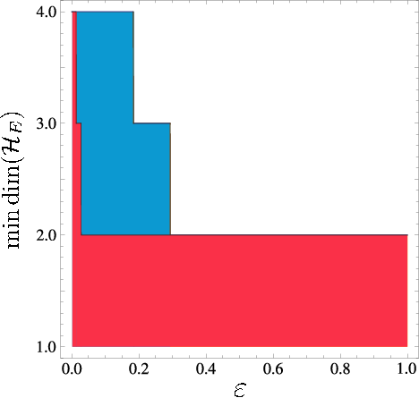
Refer to caption
Figure 2: Dimension of programmable processor in approximate programming. We consider the dimension of a processor capable of implementing the four noisy unitary channels ℰi:ϱ↦(1−ε)​σi​ϱ​σi†+ε​12​𝟙,\mathcal{E}_{i}:\varrho\mapsto(1-\varepsilon)\sigma_{i}\varrho\sigma_{i}^{\dagger}+\varepsilon\frac{1}{2}\mathbbm{1}, i=0,…,3i=0,\ldots,3, in terms of the noise parameter ε∈[0,1]\varepsilon\in[0,1]. It may be confirmed that the process fidelity satisfies Fproc​(σi⋅σi†,ℰi)≥1−εF_{\text{proc}}\big(\sigma_{i}\cdot\sigma_{i}^{\dagger},\mathcal{E}_{i}\big)\geq 1-\varepsilon for all i=0,…,3i=0,\ldots,3. Accordingly, an analysis done in Ref. [13] implies that any processor implementing ℰi\mathcal{E}_{i}, i=0,…,3i=0,\ldots,3, is at least four dimensional for 0≤ε<[3​(13+2​42)]−10\leq\varepsilon<\left[3(13+2\sqrt{42})\right]^{-1}, at least three dimensional for [3​(13+2​42)]−1≤ε<[2​(9+4​5)]−1\left[3(13+2\sqrt{42})\right]^{-1}\leq\varepsilon<\left[2(9+4\sqrt{5})\right]^{-1} and at least two dimensional for [2​(9+4​5)]−1≤ε<1\left[2(9+4\sqrt{5})\right]^{-1}\leq\varepsilon<1 excluding the dimensions within the red area. However, our approach results to tighter limits which we have denoted in blue: the processor is necessarily at least four dimensional for 0≤ε<13​(3−6)0\leq\varepsilon<\frac{1}{3}(3-\sqrt{6}), at least three dimensional for 13​(3−6)≤ε<12​(2−2)\frac{1}{3}(3-\sqrt{6})\leq\varepsilon<\frac{1}{2}(2-\sqrt{2}) and at least two dimensional for 12​(2−2)≤ε<1\frac{1}{2}(2-\sqrt{2})\leq\varepsilon<1.

Nevertheless, the channel α\alpha-fidelity ℱα\mathcal{F}_{\alpha} is a genuinely important figure of merit in quantum programming, as we will see in the following. According to the previous proposition, programming NN different unitary channels requires dim(ℋE)≥N\dim(\mathcal{H}_{E})\geq N. The processor’s dimension may, however, be lowered if some error is accepted. Let us denote d=dim(ℋS)d=\dim(\mathcal{H}_{S}). Suppose we wish to program the approximate unitary channels ℰUi​(ϱ)=(1−ε)​𝒰j​(ϱ)+ε​1d​𝟙ℋS\mathcal{E}_{U_{i}}(\varrho)=(1-\varepsilon)\mathcal{U}_{j}(\varrho)+\varepsilon\frac{1}{d}\mathbbm{1}_{\mathcal{H}_{S}} with programming vectors |ϕi⟩|\phi_{i}\rangle, respectively, where UiU_{i}, i=1,…,Ni=1,\ldots,N are unequal unitaries and ε∈[0,1]\varepsilon\in[0,1] describes a fixed error rate. From Ref. [35] we find that F1/2​(ℰUj​(ϱ1),ℰUk​(ϱ2))≤tr​[ℰUj​(ϱ1)​ℰUk​(ϱ2)]+(1−tr​[ℰUj​(ϱ1)2])​(1−tr​[ℰUk​(ϱ2)2]).F_{1/2}\big(\mathcal{E}_{U_{j}}(\varrho_{1}),\mathcal{E}_{U_{k}}(\varrho_{2})\big)\leq\textrm{tr}\left[\mathcal{E}_{U_{j}}(\varrho_{1})\,\mathcal{E}_{U_{k}}(\varrho_{2})\right]+\sqrt{\big(1-\textrm{tr}\left[\mathcal{E}_{U_{j}}(\varrho_{1})^{2}\right]\big)\big(1-\textrm{tr}\left[\mathcal{E}_{U_{k}}(\varrho_{2})^{2}\right]\big)}. Choosing ϱi=|φi⟩​⟨φi|\varrho_{i}=|\varphi_{i}\rangle\langle\varphi_{i}|, i=1,2i=1,2 simplifies this inequality yielding F1/2​(ℰUj​(ϱ1),ℰUk​(ϱ2))F1/2​(ϱ1,ϱ2)≤(1−ε)2​|⟨Uj​φ1|Uk​φ2⟩|2|⟨φ1|φ2⟩|+(2−ε)​ε|⟨φ1|φ2⟩|.\frac{F_{1/2}\big(\mathcal{E}_{U_{j}}(\varrho_{1}),\mathcal{E}_{U_{k}}(\varrho_{2})\big)}{F_{1/2}(\varrho_{1},\varrho_{2})}\leq\frac{(1-\varepsilon)^{2}|\langle U_{j}\varphi_{1}|U_{k}\varphi_{2}\rangle|^{2}}{|\langle\varphi_{1}|\varphi_{2}\rangle|}+\frac{(2-\varepsilon)\varepsilon}{|\langle\varphi_{1}|\varphi_{2}\rangle|}. In particular, choosing φ2\varphi_{2} as in Eq. (21) for U=Uj†​UkU=U_{j}^{\dagger}U_{k} implies

F1/2​(ϕj,ϕk)\displaystyle F_{1/2}(\phi_{j},\phi_{k}) ≤\displaystyle\leq inf|φ1⟩(2−ε)​ε1−|⟨Uj​φ1|Uk​φ1⟩|2\displaystyle\inf_{|\varphi_{1}\rangle}\frac{(2-\varepsilon)\varepsilon}{\sqrt{1-|\langle U_{j}\varphi_{1}|U_{k}\varphi_{1}\rangle|^{2}}}
=\displaystyle= (2−ε)​ε1−infϱF1/2​(𝒰j​(ϱ),𝒰k​(ϱ))≐gj​k​(ε),\displaystyle\frac{(2-\varepsilon)\varepsilon}{\sqrt{1-\inf_{\varrho}F_{1/2}\big(\mathcal{U}_{j}(\varrho),\mathcal{U}_{k}(\varrho)\big)}}\doteq g_{jk}(\varepsilon),

when j≠kj\neq k. We may use this bound to solve for the largest set of linearly independent programming vectors using the following result: if |ϕj⟩,j=1,…,K|\phi_{j}\rangle,\,j=1,\ldots,K, are unit vectors and F1/2​(ϕj,ϕk)≤1K−1F_{1/2}(\phi_{j},\phi_{k})\leq\frac{1}{K-1} whenever j≠kj\neq k, then the vectors |ϕj⟩,j=1,…,K|\phi_{j}\rangle,\,j=1,\ldots,K, are linearly independent [12]. Let us denote with KεK_{\varepsilon} the largest integer such that Kε<maxj≠k∈{1,…​N}⁡(1/gj​k​(ε)+1)K_{\varepsilon}<\max_{j\neq k\in\{1,\ldots N\}}\big(1/g_{jk}(\varepsilon)+1\big). The previous result then implies that any set of vectors whose size is less than or equal to KεK_{\varepsilon} is linearly independent. Therefore, if N≤KεN\leq K_{\varepsilon}, then all of the programming vectors are linearly independent and dim(ℋE)≥N\dim(\mathcal{H}_{E})\geq N. On the other hand if N>KεN>K_{\varepsilon}, then dim(ℋE)≥Kε\dim(\mathcal{H}_{E})\geq K_{\varepsilon} [13].

As an example, let us consider approximate programming of qubit unitaries σi\sigma_{i}, i=0,…,3i=0,\ldots,3, where σ0=𝟙ℂ2\sigma_{0}=\mathbbm{1}_{\mathbb{C}^{2}}. For all pairs the quantity infϱF1/2​(σj​ϱ​σj,σk​ϱ​σk)\inf_{\varrho}F_{1/2}\big(\sigma_{j}\varrho\sigma_{j},\sigma_{k}\varrho\sigma_{k}\big) vanishes. Therefore, according to Eq. (III.1) the processor in approximate programming of the above unitaries is at least four dimensional for 0≤ε<13​(3−6)0\leq\varepsilon<\frac{1}{3}(3-\sqrt{6}), at least three dimensional for 13​(3−6)≤ε<12​(2−2)\frac{1}{3}(3-\sqrt{6})\leq\varepsilon<\frac{1}{2}(2-\sqrt{2}) and at least two dimensional for 12​(2−2)≤ε<1\frac{1}{2}(2-\sqrt{2})\leq\varepsilon<1. In Fig. 2 these bounds have been compared to those previously solved in Ref. [13]. It is noteworthy that our approach gives tighter limits for the amount of noise necessary to be present in order to approximately implement the four unitary channels σi\sigma_{i}, i=0,…,3i=0,\ldots,3.

III.2 Ruling out incompatible environmental properties

Let us consider a general thermal environment ℋE\mathcal{H}_{E} and two initial states of the environment in different temperatures T1T_{1} and T2T_{2}. The environmental states therefore attain the Gibbs form ξ⁡(βi)≐exp​[−βi​𝖧E]/Z⁡(βi,𝖧E)\xi(\beta_{i})\doteq\textrm{exp}[-\beta_{i}\mathsf{H}_{E}]/Z(\beta_{i},\mathsf{H}_{E}), i=1,2i=1,2, where βi=(kB​Ti)−1\beta_{i}=(k_{B}T_{i})^{-1}, where 𝖧E\mathsf{H}_{E} is a Hamiltonian of the environment and Z⁡(βi,𝖧E)≐tr​[exp​[−βi​𝖧E]]Z(\beta_{i},\mathsf{H}_{E})\doteq\textrm{tr}\left[\textrm{exp}[-\beta_{i}\mathsf{H}_{E}]\right] are the corresponding partition functions for i=1,2i=1,2.

Our goal is to exclude some properties of environment inscribed in the spectrum of the Hamiltonian 𝖧E\mathsf{H}_{E} that are incompatible with Ineq. (19). Since for thermal states [ξ⁡(β1),ξ⁡(β2)]=0\left[\xi(\beta_{1}),\xi(\beta_{2})\right]=0, we easily solve

Sα(ξ(β1)||ξ(β2))=1α−1(ln[Z(αβ1+(1−α)β2,𝖧E)]−αln[Z(β1,𝖧E)]−(1−α)ln[Z(β2,𝖧E)]).S_{\alpha}\big(\xi(\beta_{1})||\xi(\beta_{2})\big)=\frac{1}{\alpha-1}\big(\ln\left[Z(\alpha\beta_{1}+(1-\alpha)\beta_{2},\mathsf{H}_{E})\right]-\alpha\ln\left[Z(\beta_{1},\mathsf{H}_{E})\right]-(1-\alpha)\ln\left[Z(\beta_{2},\mathsf{H}_{E})\right]\big). (24)

In particular, for all α∈[12,1)\alpha\in[\frac{1}{2},1) Ineq. (19) implies the following inequality

ln⁡[Z⁡(α​β1+(1−α)​β2,𝖧E)]−α​ln​[Z⁡(β1,𝖧E)]−(1−α)​ln​[Z⁡(β2,𝖧E)]≤inft≥0ln⁡[ℱα​(ℰ1(t),ℰ2(t))].\ln\left[Z(\alpha\beta_{1}+(1-\alpha)\beta_{2},\mathsf{H}_{E})\right]-\alpha\ln\left[Z(\beta_{1},\mathsf{H}_{E})\right]-(1-\alpha)\ln\left[Z(\beta_{2},\mathsf{H}_{E})\right]\leq\inf_{t\geq 0}\ln\left[\mathcal{F}_{\alpha}\big(\mathcal{E}_{1}^{(t)},\mathcal{E}_{2}^{(t)}\big)\right]. (25)

In fact, due to the commutativity of the thermal states, we can expand this for α∈(0,1)\alpha\in(0,1) such that

ln⁡[Z⁡(α​β1+(1−α)​β2,𝖧E)]−α​ln​[Z⁡(β1,𝖧E)]−(1−α)​ln​[Z⁡(β2,𝖧E)]≤inft≥0{ln⁡[ℱα​(ℰ2(t),ℰ1(t))],for​α∈(0,12)ln⁡[ℱα​(ℰ1(t),ℰ2(t))],for​α∈[12,1).\ln\left[Z(\alpha\beta_{1}+(1-\alpha)\beta_{2},\mathsf{H}_{E})\right]-\alpha\ln\left[Z(\beta_{1},\mathsf{H}_{E})\right]-(1-\alpha)\ln\left[Z(\beta_{2},\mathsf{H}_{E})\right]\leq\inf_{t\geq 0}\left\{\begin{array}[]{cc}\ln[\mathcal{F}_{\alpha}\big(\mathcal{E}_{2}^{(t)},\mathcal{E}_{1}^{(t)}\big)],\text{for}\ \alpha\in(0,\frac{1}{2})\\ \ln[\mathcal{F}_{\alpha}\big(\mathcal{E}_{1}^{(t)},\mathcal{E}_{2}^{(t)}\big)],\text{for}\ \alpha\in[\frac{1}{2},1)\end{array}\right.. (26)

Let us consider the implications of the above inequalities. Assume that it is possible to prepare the environment in two different known temperatures and perform the full-process tomography of the two induced dynamics. This enables us to determine the values of ℱα\mathcal{F}_{\alpha} in the right-hand side of Ineq. (26). On the other hand, any hypothesis about the Hamiltonian of the environment determines the left-hand side of the inequality. If the inequality is not satisfied, the hypothesized Hamiltonian of the system can be ruled out as incompatible with the induced pair of dynamics. We highlight that in order to do so neither the system-environment coupling nor the Hamiltonian of the system needs to be specified.

As a demonstration of the power of this method, let us consider a specific example of a qubit system coupled to an environment consisting of a single harmonic oscillator: such a situation could occur, for instance, when a two-level atom is passing through an optical cavity including only a single quantized mode. Assume that the mechanism of interaction is unknown as well as the oscillator frequency which we nevertheless wish to determine. Mathematically, we only know that the Hamiltonian of the environment is of the form 𝖧E=ω⁡(b†​b+12​𝟙)\mathsf{H}_{E}=\omega\big(b^{\dagger}b+\frac{1}{2}\mathbbm{1}\big). Choosing different values for ω\omega one plots the dashed coloured curves in Fig. 3 given by the left-hand side of Ineq. (26). For a concrete example of the (exactly solvable) reduced dynamics giving the right-hand-side of Ineq. (26) and the solid black curve in Fig. 3, we consider the interaction model of the form

𝖧\displaystyle\mathsf{H} =\displaystyle= 𝖧S+𝖧E+𝖧I\displaystyle\mathsf{H}_{S}+\mathsf{H}_{E}+\mathsf{H}_{I} (27)
=\displaystyle= ω02​σ3+ω⁡(b†​b+12​𝟙)+σ3⊗(g​b†+g∗​b)\displaystyle\frac{\omega_{0}}{2}\sigma_{3}+\omega\big(b^{\dagger}b+\frac{1}{2}\mathbbm{1}\big)+\sigma_{3}\otimes\big(gb^{\dagger}+g^{*}b\big)\,

analysed in [1]. One can see, that the inequality forbids frequency values greater than 3.1 times the real frequency ω\omega. For details we refer the reader to Appendix APPENDIX B.

Refer to caption
Figure 3: Excluding the frequency values of a harmonic oscillator. (In this example we have fixed ℏ=1=kB\hbar=1=k_{B}.) We prepare the environment in two temperatures and measure the induced dynamics, which gives us right-hand-side of Ineq. (26) (black line). The three dashed coloured lines correspond to the left-hand-side of Ineq. (26) with different choices for ωk\omega_{k}, k=1,2,3k=1,2,3, in units of the actual frequency ω\omega. Knowing the two temperatures of the environment (T1/ω=0.25T_{1}/\omega=0.25) and (T2/ω=0.75T_{2}/\omega=0.75) we notice that some frequencies (ω1/ω=3\omega_{1}/\omega=3) are compatible with Ineq. (26) while others (ω2/ω=3.1\omega_{2}/\omega=3.1 and ω3/ω=3.25\omega_{3}/\omega=3.25) violate it. In fact, we see that Ineq. (26) is violated for all frequencies larger than ω2/ω=3.1\omega_{2}/\omega=3.1, and thus ω2/ω=3.1\omega_{2}/\omega=3.1 is the crossover between the compatible and incompatible frequencies. As the probe we use a qubit and the induced dynamics result from an exactly solvable model described in [1]. The optimal initial state(s) of the qubit are ϱ=|+⟩⟨+|\varrho=|+\rangle\langle+| with |+⟩=12​(|0⟩+|1⟩)|+\rangle=\frac{1}{\sqrt{2}}(|0\rangle+|1\rangle) being the eigenstate of Pauli operator σ1\sigma_{1}; for details see Appendix B.

III.3 Quantum thermometry

Let us consider the situation of the previous example from a different perspective. Suppose now that a thermal environment described by a single harmonic oscillator with Hamiltonian 𝖧E=ω⁡(b†​b+12​𝟙)\mathsf{H}_{E}=\omega\big(b^{\dagger}b+\frac{1}{2}\mathbbm{1}\big) is initially prepared at calibration temperature T0=0T_{0}=0, that is ξ⁡(β0=∞)=|0⟩​⟨0|\xi(\beta_{0}=\infty)=|0\rangle\langle 0|. Let us assume we are tasked with probing another temperature TT of the environment. The α\alpha-Rényi divergence between the states ξ⁡(β0)\xi(\beta_{0}) and ξ⁡(β=1/(kB​T))\xi(\beta=1/(k_{B}T)) now reads Sα(ξ(β0)||ξ(β))=1−αα−1(−β​ℏ​ω2−ln[Z(β,𝖧E)])S_{\alpha}\big(\xi(\beta_{0})||\xi(\beta)\big)=\frac{1-\alpha}{\alpha-1}\big(-\frac{\beta\hbar\omega}{2}-\ln[Z(\beta,\mathsf{H}_{E})]\big) and therefore after some simple algebra we solve from Ineq.(9) a lower bound for the temperature

kB​Tℏ​ω≥\displaystyle\frac{k_{B}T}{\hbar\omega}\geq
−1×{[ln⁡[1−inft≥0ℱα​(ℰT(t),ℰ0(t))1α]]−1,α∈(0,12)[ln⁡[1−inft≥0ℱα​(ℰ0(t),ℰT(t))11−α]]−1,α∈[12,1)\displaystyle-1\times\left\{\begin{array}[]{ll}\left[\ln\left[1-\inf_{t\geq 0}\mathcal{F}_{\alpha}\big(\mathcal{E}_{T}^{(t)},\mathcal{E}_{0}^{(t)}\big)^{\frac{1}{\alpha}}\right]\right]^{-1},&\alpha\in(0,\frac{1}{2})\\ \left[\ln\left[1-\inf_{t\geq 0}\mathcal{F}_{\alpha}\big(\mathcal{E}_{0}^{(t)},\mathcal{E}_{T}^{(t)}\big)^{\frac{1}{1-\alpha}}\right]\right]^{-1},&\alpha\in[\frac{1}{2},1)\end{array}\right.

for all T≥0T\geq 0. It can be confirmed, that with temperatures lower than a limiting temperature (kB​T)/(ℏ​ω)≲1.03(k_{B}T)/(\hbar\omega)\lesssim 1.03 the term −ln⁡[Z⁡(β,𝖧E)]=β​ℏ​ω2+ln⁡[1−e−β​ℏ​ω]-\ln[Z(\beta,\mathsf{H}_{E})]=\frac{\beta\hbar\omega}{2}+\ln[1-e^{-\beta\hbar\omega}] is non-negative, from which using Ineq. (9) we may also obtain an upper bound for the temperature

kB​Tℏ​ω≤\displaystyle\frac{k_{B}T}{\hbar\omega}\leq
−1/2×{[ln⁡[inft≥0ℱα​(ℰT(t),ℰ0(t))1α]]−1,α∈(0,12)[ln⁡[inft≥0ℱα​(ℰ0(t),ℰT(t))11−α]]−1,α∈[12,1)\displaystyle-1/2\times\left\{\begin{array}[]{ll}\left[\ln\left[\inf_{t\geq 0}\mathcal{F}_{\alpha}\big(\mathcal{E}_{T}^{(t)},\mathcal{E}_{0}^{(t)}\big)^{\frac{1}{\alpha}}\right]\right]^{-1},&\alpha\in(0,\frac{1}{2})\\ \left[\ln\left[\inf_{t\geq 0}\mathcal{F}_{\alpha}\big(\mathcal{E}_{0}^{(t)},\mathcal{E}_{T}^{(t)}\big)^{\frac{1}{1-\alpha}}\right]\right]^{-1},&\alpha\in[\frac{1}{2},1)\end{array}\right.\qquad

Since there is no dependency on the parameter α\alpha on the left-hand-side of the above inequalities, we optimize over this parameter. The quantities on the right-hand-side of the inequalities above can be solved (numerically) after measuring the dynamics; these observations allow us to estimate the unknown temperature TT.

The inequalities (III.3) and (III.3) may, unfortunately, be difficult to evaluate in general due to double optimization with respect to states and therefore a more accessible form is desirable. To achieve this, we use the fact that ℱα​(ℰ1,ℰ2)≤infϱFα​(ℰ1​(ϱ),ℰ2​(ϱ))\mathcal{F}_{\alpha}\big(\mathcal{E}_{1},\mathcal{E}_{2}\big)\leq\inf_{\varrho}F_{\alpha}\big(\mathcal{E}_{1}(\varrho),\mathcal{E}_{2}(\varrho)\big), for all α∈(0,1)\alpha\in(0,1). Since Sα(⋅||⋅)S_{\alpha}(\cdot||\cdot) is monotonically increasing in α\alpha [20], that is, Sα(ϱ1||ϱ2)≤Sα′(ϱ1||ϱ2)S_{\alpha}\big(\varrho_{1}||\varrho_{2}\big)\leq S_{\alpha^{\prime}}\big(\varrho_{1}||\varrho_{2}\big) whenever α≤α′\alpha\leq\alpha^{\prime}, and since the logarithm function is monotonically increasing, we conclude that Fα​(ϱ1,ϱ2)11−αF_{\alpha}(\varrho_{1},\varrho_{2})^{\frac{1}{1-\alpha}} monotonically decreases in α\alpha. On the other hand, since for all positive semidefinite linear operators A,BA,B and numbers q≥0,r≥1q\geq 0,r\geq 1 the Araki-Lieb-Thirring inequality [36, 37] states that tr​[(B1/2​A​B1/2)r​q]≤tr​[(Br/2​Ar​Br/2)q]\textrm{tr}\left[\big(B^{1/2}AB^{1/2}\big)^{rq}\right]\leq\textrm{tr}\left[\big(B^{r/2}A^{r}B^{r/2}\big)^{q}\right] holds and since Fα​(ϱ1,ϱ2)F_{\alpha}(\varrho_{1},\varrho_{2}) may be recast in the form 22 2 This follows from the fact that the operators X​X†XX^{\dagger} and X†​XX^{\dagger}X have the same non-zero eigenvalues, and therefore tr​[(X​X†)α]=tr​[(X†​X)α]\textrm{tr}\left[(XX^{\dagger})^{\alpha}\right]=\textrm{tr}\left[(X^{\dagger}X)^{\alpha}\right]. Fα​(ϱ1,ϱ2)=tr​[(ϱ11/2​ϱ2(1−α)/α​ϱ11/2)α]F_{\alpha}(\varrho_{1},\varrho_{2})=\textrm{tr}\left[\big(\varrho_{1}^{1/2}\varrho_{2}^{(1-\alpha)/\alpha}\varrho_{1}^{1/2}\big)^{\alpha}\right], we have

Fα​(ϱ1,ϱ2)\displaystyle F_{\alpha}(\varrho_{1},\varrho_{2}) =\displaystyle= tr​[(ϱ11/2​ϱ2(1−α)/α​ϱ11/2)α1−α​(1−α)]\displaystyle\textrm{tr}\left[\big(\varrho_{1}^{1/2}\varrho_{2}^{(1-\alpha)/\alpha}\varrho_{1}^{1/2}\big)^{\frac{\alpha}{1-\alpha}(1-\alpha)}\right] (32)
≤\displaystyle\leq tr​[(ϱ1α/2​(1−α)​ϱ2​ϱ1α/2​(1−α))1−α]\displaystyle\textrm{tr}\left[\big(\varrho_{1}^{\alpha/2(1-\alpha)}\varrho_{2}\varrho_{1}^{\alpha/2(1-\alpha)}\big)^{1-\alpha}\right]
=\displaystyle= F1−α​(ϱ2,ϱ1)\displaystyle F_{1-\alpha}(\varrho_{2},\varrho_{1})

and therefore Fα​(ϱ1,ϱ2)1/(1−α)≤F1−α​(ϱ2,ϱ1)1/(1−α)F_{\alpha}(\varrho_{1},\varrho_{2})^{1/(1-\alpha)}\leq F_{1-\alpha}(\varrho_{2},\varrho_{1})^{1/(1-\alpha)} whenever α≥1/2\alpha\geq 1/2 (⇔r=α1−α≥1\Leftrightarrow r=\frac{\alpha}{1-\alpha}\geq 1). To summarize

kB​Tℏ​ω\displaystyle\frac{k_{B}T}{\hbar\omega} ≥\displaystyle\geq −ln⁡[1−infϱ,t≥0limα↗1Fα​(ℰ0(t)​(ϱ),ℰT(t)​(ϱ))11−α]−1\displaystyle-\ln\left[1-\inf_{\varrho,t\geq 0}\lim_{\alpha\nearrow 1}F_{\alpha}\big(\mathcal{E}_{0}^{(t)}(\varrho),\mathcal{E}_{T}^{(t)}(\varrho)\big)^{\frac{1}{1-\alpha}}\right]^{-1} (33)
=\displaystyle= −ln[1−e−supϱ,t≥0S1(ℰ0(t)(ϱ)||ℰT(t)(ϱ))]−1,\displaystyle-\ln\left[1-e^{-\sup_{\varrho,t\geq 0}S_{1}\big(\mathcal{E}_{0}^{(t)}(\varrho)||\mathcal{E}_{T}^{(t)}(\varrho)\big)}\right]^{-1}\,,

for T≥0T\geq 0, where limα↗1Sα(ϱ1||ϱ2)=S1(ϱ1||ϱ2)≐tr[ϱ1(lnϱ1−lnϱ2)]\lim_{\alpha\nearrow 1}S_{\alpha}(\varrho_{1}||\varrho_{2}\big)=S_{1}\big(\varrho_{1}||\varrho_{2}\big)\doteq\textrm{tr}\left[\varrho_{1}\big(\ln\varrho_{1}-\ln\varrho_{2}\big)\right] is the Kullback-Leibler divergence [20]. Similarly, for the upper bound of temperature one derives

kB​Tℏ​ω\displaystyle\frac{k_{B}T}{\hbar\omega} ≤\displaystyle\leq −1/2ln[infϱ,t≥0limα↗1Fα(ℰ0(t)(ϱ),ℰT(t)(ϱ))11−α]−1\displaystyle-1/2\ln\left[\inf_{\varrho,t\geq 0}\lim_{\alpha\nearrow 1}F_{\alpha}\big(\mathcal{E}_{0}^{(t)}(\varrho),\mathcal{E}_{T}^{(t)}(\varrho)\big)^{\frac{1}{1-\alpha}}\right]^{-1} (34)
=\displaystyle= (2supϱ,t≥0S1(ℰ0(t)(ϱ)||ℰT(t)(ϱ)))−1,\displaystyle\left(2\sup_{\varrho,t\geq 0}S_{1}\big(\mathcal{E}_{0}^{(t)}(\varrho)||\mathcal{E}_{T}^{(t)}(\varrho)\big)\right)^{-1}\,,

when 0≤(kB​T)/(ℏ​ω)≲1.03.0\leq(k_{B}T)/(\hbar\omega)\lesssim 1.03.

Refer to caption
Figure 4: Estimation of temperature. We assume that the environment is prepared in two different temperatures ((kB​T0)/(ℏ​ω)=0(k_{B}T_{0})/(\hbar\omega)=0 and (kB​T)/(ℏ​ω)(k_{B}T)/(\hbar\omega)) and measure the induced dynamics. The green line represents the actual temperature (kB​T)/(ℏ​ω)(k_{B}T)/(\hbar\omega). From Ineq. (33) we solve a lower bound of (kB​T)/(ℏ​ω)(k_{B}T)/(\hbar\omega), plotted above as the blue dashed curve. The red dotted curve corresponds to the upper bound of the temperature valid whenever (kB​T)/(ℏ​ω)≲1.03(k_{B}T)/(\hbar\omega)\lesssim 1.03 given by Ineq. (34). The system that we use for probing the temperature is a qubit and the dynamics are due to Jaynes-Cummings model in the resonant case (see Ref. [38]). The initial state of the qubit that we have used for in the plot is ϱ=|+⟩⟨+|\varrho=|+\rangle\langle+|, since numerics suggest that it leads to the optimal bounds.

In Fig. 4 we have plotted (kB​T)/(ℏ​ω)(k_{B}T)/(\hbar\omega) and the optimal bounds given by the right-hand-sides of Ineqs. (33) and (34) for the resonant Jaynes-Cummings model, which describes a two-level atom interacting with a single quantized mode of radiation in an optical cavity [1, 38]; for details we refer the reader to Appendix C. In the figure, we have chosen the initial state of the qubit probe as ϱ=|+⟩⟨+|\varrho=|+\rangle\langle+|, since numerics suggest that it leads to the optimal bounds.

A standard procedure in (quantum) thermometry is to bring the thermometer into contact with a bath, let it thermalize and then read out the temperature. In the quantum scenario, we say that a qubit probe has thermalized with the bath if any initial state ϱ\varrho of the probe evolves in the long time limit t→∞t\to\infty into the equilibrium Gibbs state ϱ→ϱeq≐(1−p⁡(T))​|0⟩​⟨0|+p⁡(T)|1⟩​⟨1|\varrho\to\varrho_{\text{eq}}\doteq\big(1-p(T)\big)\,|0\rangle\langle 0|+p(T)\,|1\rangle\langle 1|, where p⁡(T)=[1+exp​(ℏ​ω/kB​T)]−1p(T)=\big[1+\text{exp}(\hbar\omega/k_{B}T)\big]^{-1}. Quantum thermometry protocols [40, 41, 39, 42] and optimality of initial probe states [43] have been studied for both fully and partially thermalizing probes. To our best knowledge all pre-existing protocols are based on knowing the exact form of the coupling. Also the optimal initial probe states have been solved in the partially thermalized probes only for fixed system-probe couplings.

In the case of fully thermalized probes, calculating the α\alpha-fidelity becomes particularly easy: limt→∞ℱα​(ℰ0(t),ℰT(t))=(1−p⁡(T))1−α\lim_{t\to\infty}\mathcal{F}_{\alpha}\big(\mathcal{E}_{0}^{(t)},\mathcal{E}_{T}^{(t)}\big)=\big(1-p(T)\big)^{1-\alpha}. Accordingly, our protocol sets the limits

−[ln[p(T)]]−1≤kB​Tℏ​ω≤−1/2[ln[1−p(T)]]−1,\displaystyle-\big[\ln[p(T)]\big]^{-1}\leq\frac{k_{B}T}{\hbar\omega}\leq-1/2\big[\ln[1-p(T)]\big]^{-1}, (35)

with the upper bound valid whenever 0≤(kB​T)/(ℏ​ω)≲1.03.0\leq(k_{B}T)/(\hbar\omega)\lesssim 1.03. It is noteworthy, that due to the special form of the state ϱeq\varrho_{\text{eq}} the temperature TT could be solved analytically from the state occupations, which shows that our protocol is the not the optimal one for thermometry under the assumption of thermalization. However, there is no a priori need to require thermalization of the probe with the bath in our protocol. This is an important advantage, since thermalization itself in a fully quantum scenario may not be a well-defined concept due to the ever present quantum fluctuations and the long time-scales needed compared to the survival time of the quantum properties of the bath.

We wish to emphasize that knowing the specific system environment coupling is not required in the above two parameter estimation protocols B and C: to the best of our knowledge, such probing approaches independent of the description of the coupling have never been proposed before. While the precisions of the frequency estimation and thermometer are clearly not optimal, these examples serve as proofs-of-principle demonstrations of the ability to extract information on certain physical quantities by means of our approach, making only minimal assumptions on the microscopic details of the system to be probed. From a broader point of view, the two protocols B and C could be applied to estimate, not only the frequency and temperature, but also other physical quantities of a system of interest. The task to probe some of such quantities could be unattainable ”conventionally”, since the description of the coupling model between the system and the probe is not either accurately known or is borderline totally missing. An ultimate example of such case is the quantum gravity, since no commonly agreed model of gravitational interaction in quantum regime exists.

III.4 Bounds for the Loschmidt Echo

In our last application we change the perspective altogether and consider a different implication of Ineq. (12). We show how from the α\alpha-fidelity of the initial environmental states we can infer certain properties of the induced dynamics, such as information back-flow (non-Markovianity). Importantly, back-flow of information can be used to protect and restore vital quantum properties of the system subjected to detrimental noise [44, 45, 46].

As an example we concentrate on one-qubit dephasing channels arising from system environment interaction. Although the method of this subsection holds generally for such channels, we demonstrate the power of the protocol by focusing on a specific situation with known solutions only for certain initial states of environment: a qubit transversely coupled to its environment, which is an Ising spin chain in a transverse field. The total evolution of such a composite system is governed by the Hamiltonian 𝖧⁡(λ,δ)=−J​Σj​(σ3(j)⊗σ3(j+1)+λ​σ1(j)+δ⁡|e⟩​⟨e|⊗σ1(j))\mathsf{H}(\lambda,\delta)=-J\,\Sigma_{j}\big(\sigma_{3}^{(j)}\otimes\sigma_{3}^{(j+1)}+\lambda\,\sigma_{1}^{(j)}+\delta\,|e\rangle\langle e|\otimes\sigma_{1}^{(j)}\big). Here the parameters JJ, λ\lambda and δ\delta characterize the strength of the nearest neighbour interactions in the Ising chain, its coupling to a transverse field and the coupling between system and environment, respectively [47, 48]. It is known, that the initial environmental state |ϕ⟩|\phi\rangle induces dynamics corresponding to a pure dephasing channel ℰϕ(t)​(ϱ)=pϕ​(t)​ϱ+(1−pϕ​(t))​σ3​ϱ​σ3\mathcal{E}^{(t)}_{\phi}(\varrho)=p_{\phi}(t)\varrho+\big(1-p_{\phi}(t)\big)\sigma_{3}\varrho\sigma_{3} with the probability pϕ​(t)p_{\phi}(t) given by

pϕ​(t)=12​(1+Lϕ​(λ,t)),\displaystyle p_{\phi}(t)=\frac{1}{2}\big(1+\sqrt{L_{\phi}(\lambda,t)}\big), (36)

where Lϕ​(λ,t)=|⟨ϕ|ei​𝖧​(λ,0)​t​e−i​𝖧​(λ+δ,0)​t​ϕ⟩|2L_{\phi}(\lambda,t)=|\langle\phi|e^{i\mathsf{H}(\lambda,0)t}e^{-i\mathsf{H}(\lambda+\delta,0)t}\phi\rangle|^{2} is the Loschmidt echo corresponding to the state |ϕ⟩|\phi\rangle. Despite the apparent simplicity, finding an analytical expression of Lϕ​(λ,t)L_{\phi}(\lambda,t) is a difficult task for a general initial state |ϕ⟩|\phi\rangle. In fact to our best knowledge, the only known analytical solution exists for the ground state |ϕ0⟩|\phi_{0}\rangle of the Hamiltonian 𝖧⁡(λ,0)\mathsf{H}(\lambda,0) for which one obtains

Lϕ0​(λ,t)=Πk>0​(1−sin2⁡(2​αk)​sin2⁡(εk​t)),\displaystyle L_{\phi_{0}}(\lambda,t)=\Pi_{k>0}\big(1-\sin^{2}(2\alpha_{k})\sin^{2}(\varepsilon_{k}t)\big), (37)

where αk\alpha_{k} are the Bogoliubov angles and εk\varepsilon_{k} the single quasiparticle excitation energies of the system with the qubit in the excited state |e⟩|e\rangle [47, 48].

Refer to caption
Figure 5: Bounding the Loschmidt echo. (a) The dynamics of the Loschmidt echo induced by the environmental ground state ϕ0\phi_{0}. The parameter values of the Hamiltonian 𝖧⁡(λ)\mathsf{H}(\lambda) are set as J=1,δ=0.1J=1,\,\delta=0.1 and N=4000N=4000. The blue dashed line corresponds to the choice λ=0.01\lambda=0.01, the green solid line corresponds to the critical value λ=0.9\lambda=0.9 and the red dotted line corresponds to the value λ=1.8\lambda=1.8 (b) - (g) The dynamics of the upper and lower bound of the unknown Loschmidt echo are represented by the curves in lighter and darker hue of the corresponding color choices of the parameter λ\lambda, respectively. The black solid line indicates the level of the first local minimum of the upper bound. In (b) and (f) the lower bounds cross the black line after the local minimum of the upper bound, which implies revivals in the Loschmidt echo and thus information back-flow. (b) λ=0.01\lambda=0.01, F1/2​(ϕ0,ϕ)=0.98F_{1/2}(\phi_{0},\phi)=0.98. (c) λ=0.01\lambda=0.01, F1/2​(ϕ0,ϕ)=0.966675F_{1/2}(\phi_{0},\phi)=0.966675. (d) λ=0.9\lambda=0.9, F1/2​(ϕ0,ϕ)=0.98F_{1/2}(\phi_{0},\phi)=0.98. (e) λ=0.9\lambda=0.9, F1/2​(ϕ0,ϕ)=0.95F_{1/2}(\phi_{0},\phi)=0.95. (f) λ=1.8\lambda=1.8, F1/2​(ϕ0,ϕ)=0.999F_{1/2}(\phi_{0},\phi)=0.999. (g) λ=1.8\lambda=1.8, F1/2​(ϕ0,ϕ)=0.99761F_{1/2}(\phi_{0},\phi)=0.99761.

Using Ineq. (12) allows us to give an estimate for the Loschmidt echo Lϕ​(λ,t)L_{\phi}(\lambda,t) that is valid for any state |ϕ⟩|\phi\rangle. Indeed, fixing an initial state ϱ=|+⟩⟨+|\varrho=|+\rangle\langle+| of the qubit, |+⟩=12​(|0⟩+|1⟩)|+\rangle=\frac{1}{\sqrt{2}}(|0\rangle+|1\rangle) being the eigenstate of σ1\sigma_{1}, we can solve

ℰϕ(t)​(ϱ)\displaystyle\mathcal{E}^{(t)}_{\phi}(\varrho) =\displaystyle= 12​(1Lϕ​(λ,t)Lϕ​(λ,t)1).\displaystyle\frac{1}{2}\left(\begin{array}[]{cc}1&\sqrt{L_{\phi}(\lambda,t)}\\ \sqrt{L_{\phi}(\lambda,t)}&1\end{array}\right).

It can be concluded that

F1/2​(ϕ0,ϕ)\displaystyle F_{1/2}\big(\phi_{0},\phi\big) ≤F1/2​(ℰϕ0(t)​(ϱ),ℰϕ(t)​(ϱ))\displaystyle\leq F_{1/2}\big(\mathcal{E}^{(t)}_{\phi_{0}}(\varrho),\mathcal{E}^{(t)}_{\phi}(\varrho)\big)
=12​(1−Lϕ0​(λ,t))​(1−Lϕ​(λ,t))\displaystyle=\frac{1}{2}\sqrt{\big(1-\sqrt{L_{\phi_{0}}(\lambda,t)}\big)\big(1-\sqrt{L_{\phi}(\lambda,t)}\big)}
+12​(1+Lϕ0​(λ,t))​(1+Lϕ​(λ,t)),\displaystyle+\frac{1}{2}\sqrt{\big(1+\sqrt{L_{\phi_{0}}(\lambda,t)}\big)\big(1+\sqrt{L_{\phi}(\lambda,t)}\big)}, (41)

from which an estimate for Lϕ​(λ,t)L_{\phi}(\lambda,t) in terms of F1/2​(ϕ0,ϕ)F_{1/2}\big(\phi_{0},\phi\big) may be solved. In Fig. 5 we have presented the results for three different values of the strength of the transverse field λ\lambda fixing the parameters δ=0.1\delta=0.1, J=1J=1 and the number of spins N=4000N=4000. In particular, we see that for those λ\lambda resulting to revivals in Loschmidt echo in the ground state |ϕ0⟩|\phi_{0}\rangle, after a certain limiting value of Flim≤F1/2​(ϕ0,ϕ)F_{\text{lim}}\leq F_{1/2}\big(\phi_{0},\phi\big) such revivals are guaranteed for the state |ϕ⟩|\phi\rangle also. The revivals of Loschmidt echo are linked to revivals of coherences via Eq. (III.4) and hence indicate back-flow of information from environment to system.

It should be pointed out, that the upper and lower bounds of the Loschmidt echo LϕL_{\phi} could be made tighter by considering general α\alpha-fidelities in the above Ineq. (41). However, since solving LϕL_{\phi} from Ineq. (41) in such a general situation can only be done numerically, we have left this examination as a topic for future investigation.

IV Conclusions and Outlook

In this paper we have introduced a novel family of α\alpha-fidelities of quantum channels. We also have derived an inequality between the α\alpha-fidelity of the initial states of the environment and the α\alpha-fidelity of the corresponding induced dynamics: Fα​(ξ1,ξ2)≤ℱα​(ℰ1(t),ℰ2(t))F_{\alpha}(\xi_{1},\xi_{2})\leq\mathcal{F}_{\alpha}\big(\mathcal{E}_{1}^{(t)},\mathcal{E}_{2}^{(t)}\big), α∈[1/2,1)\alpha\in[1/2,1). From a more practical viewpoint, the inequality was then considered in the context of four different applications: A) quantum programming, B) discrimination of environmental properties, C) quantum thermometry and in D) deriving bounds for the Loschmidt echo of a general (pure) initial state of the spin-chain.

In a nutshell, the general procedure of estimating an unknown ξ2\xi_{2} requires 1) the possibility to prepare the environment in a known ”calibration” state ξ1\xi_{1} and 2) the possibility to compare the probe dynamic ℰ1(t)\mathcal{E}_{1}^{(t)} and ℰ2(t)\mathcal{E}_{2}^{(t)} induced by these states. To apply our framework to quantum probing experimentally, as proposed in examples B), C) and D), the experimenter needs first to perform quantum process tomography and then numerical optimization for all times, which may be extremely difficult. However, the starting point underlying behind our results is the Ineq. (12), which shows that non-trivial bounds for Fα​(ξ1,ξ2)F_{\alpha}(\xi_{1},\xi_{2}) may be found for plethora of choices of initial probe states ϱ1\varrho_{1} and ϱ2\varrho_{2}; the notion of α\alpha-fidelity of dynamics was developed as the best achievable resolution of this inequality. In particular, choosing ϱi=ϱ,\varrho_{i}=\varrho, i=1,2i=1,2, simplifies the Ineq. (12) to

Fα​(ξ1,ξ2)≤Fα​(ℰ1(t)​(ϱ),ℰ2(t)​(ϱ))≤1,\displaystyle F_{\alpha}(\xi_{1},\xi_{2})\leq F_{\alpha}\big(\mathcal{E}_{1}^{(t)}(\varrho),\mathcal{E}_{2}^{(t)}(\varrho)\big)\leq 1\,, (42)

for all ϱ∈𝒮⁡(ℋS)\varrho\in\mathcal{S}(\mathcal{H}_{S}) and α∈[1/2,1)\alpha\in[1/2,1) and any given time t∈[0,∞)t\in[0,\infty). Although the resulting upper bound Fα​(ℰ1​(ϱ),ℰ2​(ϱ))F_{\alpha}\big(\mathcal{E}_{1}(\varrho),\mathcal{E}_{2}(\varrho)\big) may not be the optimal one, any choice of the initial state of ϱ∈𝒮⁡(ℋS)\varrho\in\mathcal{S}(\mathcal{H}_{S}) allows one to extract some information of system of interest via the protocols described above. In addition, the full process tomography is now reduced from the full channel tomography to mere state tomography of the evolved states of the probe ℰ1​(ϱ)\mathcal{E}_{1}(\varrho) and ℰ2​(ϱ)\mathcal{E}_{2}(\varrho).

In our theoretical framework the introduced fidelities are based on the definition of the α\alpha-Rényi divergence, given in Eq. (II), mainly because of its connection to the Uhlmann fidelity for α=1/2\alpha=1/2. However as we mentioned before, there exists another quantum divergence often encountered in the literature, namely S~α\widetilde{S}_{\alpha} defined in Eq.(II). It is known that also S~α\widetilde{S}_{\alpha} satisfies both the properties (S1)-(S3) and the data processing inequality (S4) for all α∈(0,1)\alpha\in(0,1) [20]. Hence, also for F~α​(ϱ1,ϱ2)≐tr​[ϱ1α​ϱ21−α]\widetilde{F}_{\alpha}(\varrho_{1},\varrho_{2})\doteq\textrm{tr}\left[\varrho_{1}^{\alpha}\varrho_{2}^{1-\alpha}\right], we have F~α​(ϱ1,ϱ2)​F~α​(ξ1,ξ2)≤F~α​(ℰ1(t)​(ϱ1),ℰ2(t)​(ϱ2))\widetilde{F}_{\alpha}(\varrho_{1},\varrho_{2})\widetilde{F}_{\alpha}(\xi_{1},\xi_{2})\leq\widetilde{F}_{\alpha}\big(\mathcal{E}_{1}^{(t)}(\varrho_{1}),\mathcal{E}_{2}^{(t)}(\varrho_{2})\big), α∈(0,1)\alpha\in(0,1). Furthermore, for commuting states [ϱ1,ϱ2]=0[\varrho_{1},\varrho_{2}]=0 the quantities SαS_{\alpha} and S~α\widetilde{S}_{\alpha} coincide [20]. Although it is known that F~α≤Fα\widetilde{F}_{\alpha}\leq F_{\alpha}, since Sα≤S~αS_{\alpha}\leq\widetilde{S}_{\alpha} [21, 23], an interesting question to investigate in the future is which of the two definitions F~α\widetilde{F}_{\alpha} or FαF_{\alpha} leads to a tighter inequality between the inducing states and induced dynamics – or whether such optimality even holds in general. It is noteworthy, that the results shown in Figs. 3, 4 and 5 are independent of the choice of F~α\widetilde{F}_{\alpha} or FαF_{\alpha} due to the facts that the time-evolved final states of the probe are commuting in all the three cases as well as the environment states in applications B), C), and since F~α\widetilde{F}_{\alpha} and FαF_{\alpha} coincide when comparing pure states in D).

Due to the generality of our formalism, our results can be used in different fields of physics: from quantum information theory to solid state physics, from particle physics to cosmology, from quantum gravity to atomic and molecular physics, and from quantum optics to quantum thermodynamics. Therefore our approach has the potential to pave the way to new fundamental theoretical and experimental discoveries in numerous physical scenarios.

Acknowledgements

The authors are grateful to Mário Ziman for his comments on the manuscript. S.M was supported by the EU Collaborative project QuProCS (Grant Agreement 641277) and the Academy of Finland (Project no. 287750). M.T. and H.L. acknowledge financial support from the University of Turku Graduate School (UTUGS) and M.T. additionally acknowledges the hospitality of Mathematical Physics Group in Toruń. G.S. was partially supported by the National Science Centre (project 2015/17/B/ST2/02026), the Magnus Ehrnrooth Foundation and wishes to acknowledge the hospitality of Turku Quantum Technology Group.

APPENDIX A: Evaluating α\alpha-fidelity of qubit channels

In this section we present the method that has been used to evaluate the α\alpha-fidelity of one-qubit channels. First we simplify the analytic expression to make the numeric optimization more feasible. The density matrices of two arbitrary one-qubit states ϱk\varrho_{k}, k=1,2k=1,2, can be written in the Bloch form as

ϱk\displaystyle\varrho_{k} =\displaystyle= 12​(𝟙+xk​σ1+yk​σ2+zk​σ3)\displaystyle\frac{1}{2}\left(\mathbbm{1}+x_{k}\sigma_{1}+y_{k}\sigma_{2}+z_{k}\sigma_{3}\right)
=\displaystyle= 12​(1+zkxk−i​ykxk+i​yk1−zk),\displaystyle\frac{1}{2}\left(\begin{array}[]{cc}1+z_{k}&x_{k}-iy_{k}\\ x_{k}+iy_{k}&1-z_{k}\end{array}\right)\,,

where xk,ykx_{k},\,y_{k} and zkz_{k} are real numbers satisfying xk2+yk2+zk2≤1x_{k}^{2}+y_{k}^{2}+z_{k}^{2}\leq 1 and σ1,σ2\sigma_{1},\,\sigma_{2} and σ3\sigma_{3} are the Pauli operators. The density matrices can be diagonalized as

ϱk=12​rk​(rk+zk)(rk+zk−(xk−i​yk)xk+i​ykrk+zk)×\displaystyle\varrho_{k}=\frac{1}{2r_{k}(r_{k}+z_{k})}\left(\begin{array}[]{cc}r_{k}+z_{k}&-(x_{k}-iy_{k})\\ x_{k}+iy_{k}&r_{k}+z_{k}\end{array}\right)\times
(1+rk2001−rk2)​(rk+zk−(xk−i​yk)xk+i​ykrk+zk)†,\displaystyle\left(\begin{array}[]{cc}\frac{1+r_{k}}{2}&0\\ 0&\frac{1-r_{k}}{2}\end{array}\right)\left(\begin{array}[]{cc}r_{k}+z_{k}&-(x_{k}-iy_{k})\\ x_{k}+iy_{k}&r_{k}+z_{k}\end{array}\right)^{\dagger},

where rk=xk2+yk2+zk2r_{k}=\sqrt{x_{k}^{2}+y_{k}^{2}+z_{k}^{2}}. Now by using Eq. (APPENDIX A: Evaluating α\alpha-fidelity of qubit channels) we can simplify the form of ϱk1−αα\varrho_{k}^{\frac{1-\alpha}{\alpha}} as

ϱk1−αα=12​rk​(rk​Ak++zk​Ak−(xk−i​yk)​Ak−(xk+i​yk)​A−rk​Ak+−zk​Ak−),\varrho_{k}^{\frac{1-\alpha}{\alpha}}=\frac{1}{2r_{k}}\left(\begin{array}[]{cc}r_{k}A_{k}^{+}+z_{k}A_{k}^{-}&(x_{k}-iy_{k})A_{k}^{-}\\ (x_{k}+iy_{k})A^{-}&r_{k}A_{k}^{+}-z_{k}A_{k}^{-}\end{array}\right), (54)

where Ak±=(1+rk2)1−αα±(1−rk2)1−ααA_{k}^{\pm}=\left(\frac{1+r_{k}}{2}\right)^{\frac{1-\alpha}{\alpha}}\pm\left(\frac{1-r_{k}}{2}\right)^{\frac{1-\alpha}{\alpha}}. By using Eq. (54) and the properties of trace and determinant, we can calculate the trace and determinant of the matrix product ϱ21−α2​α​ϱ1​ϱ21−α2​α\varrho_{2}^{\frac{1-\alpha}{2\alpha}}\varrho_{1}\varrho_{2}^{\frac{1-\alpha}{2\alpha}} as

T\displaystyle T :⁣=\displaystyle:= tr​[ϱ21−α2​α​ϱ1​ϱ21−α2​α]=12​A2++12​A2−​r1​r2r2,\displaystyle\text{tr}\left[\varrho_{2}^{\frac{1-\alpha}{2\alpha}}\varrho_{1}\varrho_{2}^{\frac{1-\alpha}{2\alpha}}\right]=\frac{1}{2}A^{+}_{2}+\frac{1}{2}A^{-}_{2}\frac{r_{1}r_{2}}{r_{2}}\,, (55)
D\displaystyle D :⁣=\displaystyle:= det(ϱ21−α2​α​ϱ1​ϱ21−α2​α)=(1−r224)1−αα​(1−r124).\displaystyle\det\left(\varrho_{2}^{\frac{1-\alpha}{2\alpha}}\varrho_{1}\varrho_{2}^{\frac{1-\alpha}{2\alpha}}\right)=\left(\frac{1-r_{2}^{2}}{4}\right)^{\frac{1-\alpha}{\alpha}}\left(\frac{1-r_{1}^{2}}{4}\right)\,.\qquad (56)

From Eqs. (55) and (56) we can write the eigenvalues λ+\lambda_{+} and λ−\lambda_{-} of ϱ21−α2​α​ϱ1​ϱ21−α2​α\varrho_{2}^{\frac{1-\alpha}{2\alpha}}\varrho_{1}\varrho_{2}^{\frac{1-\alpha}{2\alpha}} as

λ±=12​(T±T2−4​D).\lambda_{\pm}=\frac{1}{2}\left(T\pm\sqrt{T^{2}-4D}\right). (57)

Using these eigenvalues, we can diagonalize ϱ21−α2​α​ϱ1​ϱ21−α2​α\varrho_{2}^{\frac{1-\alpha}{2\alpha}}\varrho_{1}\varrho_{2}^{\frac{1-\alpha}{2\alpha}} as

ϱ21−α2​α​ϱ1​ϱ21−α2​α=U​R​U†,\varrho_{2}^{\frac{1-\alpha}{2\alpha}}\varrho_{1}\varrho_{2}^{\frac{1-\alpha}{2\alpha}}=URU^{\dagger}\,, (58)

where R=R= diag(λ+,λ−\lambda_{+},\lambda_{-}) and UU is the diagonalizing unitary matrix found in the same way as in Eq. (APPENDIX A: Evaluating α\alpha-fidelity of qubit channels). Finally, this allows us to express the α\alpha-fidelity of two arbitrary one-qubit states, ϱ1\varrho_{1} and ϱ2\varrho_{2}, as

Fα​(ϱ1,ϱ2)=tr​[(U​R​U†)α]=λ+α+λ−α.F_{\alpha}(\varrho_{1},\varrho_{2})=\text{tr}\left[\left(URU^{\dagger}\right)^{\alpha}\right]=\lambda_{+}^{\alpha}+\lambda_{-}^{\alpha}\,. (59)

Now we see that, in order to calculate the channel α\alpha-fidelity of one-qubit channels ℰ1\mathcal{E}_{1} and ℰ2\mathcal{E}_{2}, it is enough to minimize the quotient

Fα​(ℰ1​(ϱ1),ℰ2​(ϱ2))Fα​(ϱ1,ϱ2)=λ~+α+λ~−αλ+α+λ−α.\frac{F_{\alpha}\big(\mathcal{E}_{1}(\varrho_{1}),\mathcal{E}_{2}(\varrho_{2})\big)}{F_{\alpha}(\varrho_{1},\varrho_{2})}=\frac{\widetilde{\lambda}^{\alpha}_{+}+\widetilde{\lambda}_{-}^{\alpha}}{\lambda_{+}^{\alpha}+\lambda_{-}^{\alpha}}\,. (60)

Here λ~±\widetilde{\lambda}_{\pm} are eigenvalues of ℰ2​(ϱ2)1−α2​α​ℰ1​(ϱ1)​ℰ2​(ϱ2)1−α2​α\mathcal{E}_{2}(\varrho_{2})^{\frac{1-\alpha}{2\alpha}}\mathcal{E}_{1}(\varrho_{1})\mathcal{E}_{2}(\varrho_{2})^{\frac{1-\alpha}{2\alpha}} calculated in a similar way from the Bloch coordinates of ℰ1​(ϱ1)\mathcal{E}_{1}(\varrho_{1}) and ℰ2​(ϱ2)\mathcal{E}_{2}(\varrho_{2}), and λ±\lambda_{\pm} are the above solved eigenvalues of ϱ21−α2​α​ϱ1​ϱ21−α2​α\varrho_{2}^{\frac{1-\alpha}{2\alpha}}\varrho_{1}\varrho_{2}^{\frac{1-\alpha}{2\alpha}}, where ϱ1\varrho_{1} and ϱ2\varrho_{2} are the initial states of the qubits. The quantity to be minimized in Eq. (60) is a function of six variables x1,y1,z1,x2,y2,z2x_{1},y_{1},z_{1},x_{2},y_{2},z_{2} under the constraints x12+y12+z12≤1x_{1}^{2}+y_{1}^{2}+z_{1}^{2}\leq 1 and x22+y22+z22≤1x_{2}^{2}+y_{2}^{2}+z_{2}^{2}\leq 1.

Example: the case of pure dephasing channels

In this example the reduced dynamics is a family of dephasing channels with the same invariance basis for all values of time tt and the inverse temperature β=1/kB​T\beta=1/k_{B}T. Let Γ1​(t)\Gamma_{1}(t) and Γ2​(t)\Gamma_{2}(t) be the decoherence rates at time tt (the same for both channels) corresponding to β1\beta_{1} and β2\beta_{2}, respectively. The two dephasing channels ℰi\mathcal{E}_{i} are defined via

ϱ=12​(1+zx−i​yx+i​y1−z)\displaystyle\varrho=\frac{1}{2}\left(\begin{array}[]{cc}1+z&x-iy\\ x+iy&1-z\end{array}\right)
↦\displaystyle\mapsto ℰi(t)​(ϱ)=12​(1+zΓi​(t)​(x−i​y)Γi​(t)∗​(x+i​y)1−z).\displaystyle\mathcal{E}_{i}^{(t)}(\varrho)=\frac{1}{2}\left(\begin{array}[]{cc}1+z&\Gamma_{i}(t)(x-iy)\\ \Gamma_{i}(t)^{*}(x+iy)&1-z\end{array}\right)\,.\qquad

We have performed the numerical minimization of Eq. (60) by tools of constrained minimisation. More precisely, we have used the method SLSQP (Sequential Least Square Programming) implemented in scipy.optimize library. The numerical calculation shows, that the minimum is attained when ϱ1=ϱ2\varrho_{1}=\varrho_{2} is any pure state maximally unbiased with respect to the invariant basis, for example |+⟩⟨+|=12(𝟙+σ1)|+\rangle\langle+|=\frac{1}{2}(\mathbbm{1}+\sigma_{1}). This observation lets us write the explicit formula for α\alpha-fidelity of the dynamics:

ℱα​(ℰ1(t),ℰ2(t))\displaystyle\mathcal{F}_{\alpha}(\mathcal{E}_{1}^{(t)},\mathcal{E}_{2}^{(t)}) =\displaystyle= (1+Γ2​(t)2)1−α​(1+Γ1​(t)2)α\displaystyle\left(\frac{1+\Gamma_{2}(t)}{2}\right)^{1-\alpha}\left(\frac{1+\Gamma_{1}(t)}{2}\right)^{\alpha} (67)
+\displaystyle+ (1−Γ2​(t)2)1−α​(1−Γ1​(t)2)α.\displaystyle\left(\frac{1-\Gamma_{2}(t)}{2}\right)^{1-\alpha}\left(\frac{1-\Gamma_{1}(t)}{2}\right)^{\alpha}.\qquad

APPENDIX B

In application B) (Ruling out incompatible environmental properties) we consider a system coupled to a thermal environment with Hamiltonian 𝖧E\mathsf{H}_{E} in two different inverse temperatures βi=1/Ti\beta_{i}=1/T_{i}, i=1,2i=1,2; we have used natural units ℏ=1=kB\hbar=1=k_{B} throughout this section. We showed that the partition functions Z⁡(βi,𝖧E)Z(\beta_{i},\mathsf{H}_{E}) of the two environmental states and the corresponding induced dynamics ℰi(t)\mathcal{E}_{i}^{(t)} satisfy the inequality Ineq. (26). It was reasoned that some of the properties of the environment inscribed in 𝖧E\mathsf{H}_{E} may be ruled out by measuring the dynamics induced by two different temperatures and by testing which partition functions are (in)compatible with Ineq. (26). In a particular case of environment consisting of harmonic oscillators, that is 𝖧E=∑kωk​(bk†​bk+12​𝟙)\mathsf{H}_{E}=\sum_{k}\omega_{k}\big(b_{k}^{\dagger}b_{k}+\frac{1}{2}\mathbbm{1}\big), where bk†b^{\dagger}_{k} and bkb_{k} are the creation and annihilation operators of the environmental mode kk, respectively, the logarithms of the partition functions attain a simple form

ln⁡[Z⁡(βi,𝖧E)]=∑k(−βi​ωk2−ln⁡[1−e−βi​ωk]),\displaystyle\ln\left[Z(\beta_{i},\mathsf{H}_{E})\right]=\sum_{k}\,\big(-\frac{\beta_{i}\omega_{k}}{2}-\ln\left[1-e^{-\beta_{i}\omega_{k}}\right]\big)\,,\qquad (68)

i=1,2,i=1,2, which then only depends on the oscillators frequencies ωk\omega_{k} and the known inverse temperatures βi\beta_{i}.

Inequality  (26) holds regardless of the choice of the actual coupling between the system and the environment. As an example of our method, in Fig. 3 we have, however, deployed a particular exactly solvable system-environment model leading to the dephasing channel of the system described in Ref. [1]. In this model the system is a qubit coupled to environment consisting of harmonic oscillators and the total Hamiltonian, consisting of the Hamiltonians of the system 𝖧S\mathsf{H}_{S}, the environment 𝖧E\mathsf{H}_{E}, and the interaction Hamiltonian 𝖧I\mathsf{H}_{I}, governing the composite evolution can be written as

𝖧\displaystyle\mathsf{H} =𝖧S+𝖧E+𝖧I\displaystyle=\mathsf{H}_{S}+\mathsf{H}_{E}+\mathsf{H}_{I}
=ω02​σ3+∑kωk​(bk†​bk+12​𝟙)+∑kσ3⊗(gk​bk†+gk∗​bk),\displaystyle=\frac{\omega_{0}}{2}\sigma_{3}+\sum_{k}\omega_{k}\big(b_{k}^{\dagger}b_{k}+\frac{1}{2}\mathbbm{1}\big)+\sum_{k}\sigma_{3}\otimes\big(g_{k}b_{k}^{\dagger}+g_{k}^{*}b_{k}\big)\,, (69)

gkg_{k} describes the strength at which the system couples to different modes. Fixing the initial composite system state as ϱS+E=ϱ⊗ξ⁡(βi)\varrho_{S+E}=\varrho\otimes\xi(\beta_{i}) we get an analytical solution for the qubit system dynamics

ϱ=(ϱ00ϱ01ϱ10ϱ11)↦ℰi(t)​(ϱ)=(ϱ00Γi​(t)​ϱ01Γi​(t)​ϱ10ϱ11),\varrho=\begin{pmatrix}\varrho_{00}&\varrho_{01}\\ \varrho_{10}&\varrho_{11}\end{pmatrix}\mapsto\mathcal{E}_{i}^{(t)}(\varrho)=\begin{pmatrix}\varrho_{00}&\Gamma_{i}(t)\,\varrho_{01}\\ \Gamma_{i}(t)\,\varrho_{10}&\varrho_{11}\end{pmatrix}\,, (70)

where Γi(t)=exp[−∑k4​|gk|2ωk2coth(ωk2​Ti)[1−cos(ωkt)]]\Gamma_{i}(t)=\text{exp}\big[-\sum_{k}\frac{4|g_{k}|^{2}}{\omega_{k}^{2}}\coth\big(\frac{\omega_{k}}{2T_{i}}\big)\big[1-\cos(\omega_{k}t)\big]\big]; we refer the reader to [1] for further details of this model.

For simplicity we will only consider environment consisting of a single oscillator; this is also the case in Fig. 3. By fixing two temperatures of the environmental initial state, T1,T2T_{1},\,T_{2}, and a single oscillator frequency ω\omega which we want to probe, we obtain two dephasing channels ℰ1(t)\mathcal{E}_{1}^{(t)} and ℰ2(t)\mathcal{E}_{2}^{(t)} of the form Eq. (70) and according to (67) their α\alpha-fidelity is equal to

ℱα​(ℰ1(t),ℰ2(t))=\displaystyle\mathcal{F}_{\alpha}(\mathcal{E}^{(t)}_{1},\mathcal{E}^{(t)}_{2})=
(1+Cg​(t)coth⁡(12​ω​β2)2)1−α​(1+Cg​(t)coth⁡(12​ω​β1)2)α\displaystyle\left(\frac{1+C_{g}(t)^{\coth(\frac{1}{2}\omega\beta_{2})}}{2}\right)^{1-\alpha}\left(\frac{1+C_{g}(t)^{\coth(\frac{1}{2}\omega\beta_{1})}}{2}\right)^{\alpha}
+\displaystyle+ (1−Cg​(t)coth⁡(12​ω​β2)2)1−α​(1−Cg​(t)coth⁡(12​ω​β1)2)α,\displaystyle\left(\frac{1-C_{g}(t)^{\coth(\frac{1}{2}\omega\beta_{2})}}{2}\right)^{1-\alpha}\left(\frac{1-C_{g}(t)^{\coth(\frac{1}{2}\omega\beta_{1})}}{2}\right)^{\alpha},

for Cg​(t)=exp⁡[−4​|g|2ω2​[1−cos⁡ω​t]]C_{g}(t)=\exp\big[-\frac{4|g|^{2}}{\omega^{2}}\big[1-\cos{\omega t}\big]\big]. Importantly, the function Cg​(t)C_{g}(t) is the only term involving both the coupling strength gg and time tt. It is easily verified that for any |g|/ω≥1/8|g|/\omega\geq 1/\sqrt{8} the function Cg​(t)C_{g}(t) can be kept constant in value by choosing tt appropriately. Therefore, we can conclude that any coupling (in units of ω\omega) stronger than 1/81/\sqrt{8} can only make the number inftℱα​(ℰ1(t),ℰ2(t))\inf_{t}\mathcal{F}_{\alpha}(\mathcal{E}^{(t)}_{1},\mathcal{E}^{(t)}_{2}) smaller and consequently our protocol to work better. For demonstration we have chosen |g|/ω=1|g|/\omega=1, T1/ω=0.25T_{1}/\omega=0.25 and T2/ω=0.75T_{2}/\omega=0.75. We can therefore plot inftln⁡[ℱα​(ℰ1(t),ℰ2(t))]\inf_{t}\ln\big[\mathcal{F}_{\alpha}(\mathcal{E}^{(t)}_{1},\mathcal{E}^{(t)}_{2})\big] as a function of α\alpha, which is the r.h.s. of Ineq. (26). Also, by using the same temperatures T1,T2T_{1},\,T_{2} and varying the frequency value in Eq. (68) we can plot the l.h.s. of Ineq. (26) as a function of α\alpha and compare it with the plot of the r.h.s. Whenever we see violation of Ineq. (26), we know that these frequency values cannot have lead to the induced dynamics. In accordance, plots with frequencies satisfying and violating Ineq. (26) are presented in Fig. 3.

APPENDIX C

In application C) (Quantum thermometry) we continue on considering a system coupled to a thermal environment. This time we assume to know the oscillator frequencies of the Hamiltonian 𝖧E=∑kωk​(bk†​bk+12​𝟙)\mathsf{H}_{E}=\sum_{k}\omega_{k}\big(b_{k}^{\dagger}b_{k}+\frac{1}{2}\mathbbm{1}\big) and again we check the induced dynamics for two different temperatures: T0=0T_{0}=0 and TT that is unknown. Since ξ⁡(∞)=⨂k|0⟩​⟨0|\xi(\infty)=\bigotimes_{k}|0\rangle\langle 0|, the α\alpha-Rényi divergence between the initial states of the environment in the inverse temperatures β0=∞\beta_{0}=\infty and β=1/kB​T\beta=1/k_{B}T can be calculated that

Sα​(ξ⁡(β0),ξ⁡(β))\displaystyle S_{\alpha}\big(\xi(\beta_{0}),\xi(\beta)\big) (72)
=\displaystyle= 1α−1​ln⁡[tr​[(ξ​(β)1−α2​α​ξ​(β0)​ξ​(β)1−α2​α)α]]\displaystyle\frac{1}{\alpha-1}\ln\left[\textrm{tr}\left[\left(\xi(\beta)^{\frac{1-\alpha}{2\alpha}}\,\xi(\beta_{0})\,\xi(\beta)^{\frac{1-\alpha}{2\alpha}}\right)^{\alpha}\right]\right]
=\displaystyle= 1−αα−1ln[e−12∑kβℏωk/Z(β,𝖧E)]\displaystyle\frac{1-\alpha}{\alpha-1}\ln\left[e^{-\frac{1}{2}\sum_{k}\beta\hbar\omega_{k}}/Z(\beta,\mathsf{H}_{E})\right]
=\displaystyle= 1−αα−1​ln⁡[∏k(1−e−β​ℏ​ωk)],\displaystyle\frac{1-\alpha}{\alpha-1}\ln\left[\prod_{k}\big(1-e^{-\beta\hbar\omega_{k}}\big)\right]\,,

with β=1/kB​T\beta=1/k_{B}T and the last equality follows from inserting Z⁡(β,𝖧E)Z(\beta,\mathsf{H}_{E}) from Eq. (68). Similarly, we confirm that

Sα​(ξ⁡(β),ξ⁡(β0))\displaystyle S_{\alpha}\big(\xi(\beta),\xi(\beta_{0})\big) =\displaystyle= αα−1​ln⁡[∏k(1−e−β​ωk)].\displaystyle\frac{\alpha}{\alpha-1}\ln\left[\prod_{k}\big(1-e^{-\beta\omega_{k}}\big)\right]\,. (73)

Consequently, from Ineq. (9) one confirms that

∏k(1−e−ℏωk/kBT)\displaystyle\prod_{k}\,\big(1-e^{-\hbar\omega_{k}/k_{B}T}\big)
≤\displaystyle\leq inft≥0{ℱα​(ℰT(t),ℰ0(t))1α,for​α∈(0,12)ℱα​(ℰ0(t),ℰT(t))11−α,for​α∈[12,1),\displaystyle\inf_{t\geq 0}\left\{\begin{array}[]{lc}\mathcal{F}_{\alpha}\big(\mathcal{E}_{T}^{(t)},\mathcal{E}_{0}^{(t)}\big)^{\frac{1}{\alpha}},&\text{for}\ \alpha\in(0,\frac{1}{2})\\ \mathcal{F}_{\alpha}\big(\mathcal{E}_{0}^{(t)},\mathcal{E}_{T}^{(t)}\big)^{\frac{1}{1-\alpha}},&\text{for}\ \alpha\in[\frac{1}{2},1)\end{array}\right.,

where ℰ0(t)\mathcal{E}_{0}^{(t)} and ℰT(t)\mathcal{E}_{T}^{(t)} are the dynamics induced by β0\beta_{0} and βT\beta_{T}, respectively. From this inequality the temperature TT can be numerically estimated. For simplicity, we again consider the case of only a single harmonic oscillator mode. In this case the above relation can be solved in terms of the temperature TT analytically: the solution is presented in Ineq. (III.3).

Notice, that the above Ineq. (APPENDIX C) holds model-independently even without a priori knowledge of the coupling between the system and the environment. As a concrete example, in Fig. 4 we have demonstrated the power of our method by considering the Jaynes-Cummings -model of a qubit coupled to a thermal environment consisting of a single harmonic oscillator. In such a model the total Hamiltonian of the system-environment composite reads

𝖧\displaystyle\mathsf{H} =\displaystyle= 𝖧S+𝖧E+𝖧I\displaystyle\mathsf{H}_{S}+\mathsf{H}_{E}+\mathsf{H}_{I} (77)
=\displaystyle= ω0​σ+​σ−+ω⁡(b†​b+12​𝟙)+g⁡(σ+⊗b+σ−⊗b†),\displaystyle\omega_{0}\sigma_{+}\sigma_{-}+\omega\big(b^{\dagger}b+\frac{1}{2}\mathbbm{1}\big)+g\big(\sigma_{+}\otimes b+\sigma_{-}\otimes b^{\dagger}\big)\,,\qquad

where σ+=|1⟩​⟨0|\sigma_{+}=|1\rangle\langle 0| and σ−=|0⟩​⟨1|\sigma_{-}=|0\rangle\langle 1| are the raising and lowering operators of the qubit system, respectively, and gg describes the coupling strength. Assume that an initial separable state of the composite system ϱ⊗ξ⁡(β)\varrho\otimes\xi(\beta) evolves according to this Hamiltonian. Then, in the resonant case of matching system and environment frequencies Δ=ω−ω0=0\Delta=\omega-\omega_{0}=0, the reduced dynamics take a relatively simple form

ϱ=(ϱ00ϱ01ϱ10ϱ11)↦ℰT(t)​(ϱ)=\displaystyle\varrho=\left(\begin{array}[]{lc}\varrho_{00}&\varrho_{01}\\ \varrho_{10}&\varrho_{11}\end{array}\right)\mapsto\mathcal{E}_{T}^{(t)}(\varrho)=
(aT​(t)​ϱ00+[1−bT​(t)]​ϱ11cT​(t)∗​ϱ01cT​(t)​ϱ10[1−aT​(t)]​ϱ00+bT​(t)​ϱ11),\displaystyle\left(\begin{array}[]{lc}a_{T}(t)\,\varrho_{00}+\big[1-b_{T}(t)\big]\,\varrho_{11}&c_{T}(t)^{*}\,\varrho_{01}\\ c_{T}(t)\,\varrho_{10}&\big[1-a_{T}(t)\big]\,\varrho_{00}+b_{T}(t)\,\varrho_{11}\end{array}\right),

where the coefficients

aT​(t)\displaystyle a_{T}(t) =\displaystyle= tr​[𝖢†​(n^,t)​𝖢​(n^,t)​ξ​(β)],\displaystyle\textrm{tr}\left[\mathsf{C}^{\dagger}(\hat{n},t)\mathsf{C}(\hat{n},t)\,\xi(\beta)\right]\,,
bT​(t)\displaystyle b_{T}(t) =\displaystyle= tr​[𝖢†​(n^+1,t)​𝖢​(n^+1,t)​ξ​(β)],\displaystyle\textrm{tr}\left[\mathsf{C}^{\dagger}(\hat{n}+1,t)\mathsf{C}(\hat{n}+1,t)\,\xi(\beta)\right]\,,
cT​(t)\displaystyle c_{T}(t) =\displaystyle= tr​[𝖢⁡(n^+1,t)​𝖢​(n^,t)​ξ​(β)]\displaystyle\textrm{tr}\left[\mathsf{C}(\hat{n}+1,t)\mathsf{C}(\hat{n},t)\,\xi(\beta)\right] (85)

depend on the operator 𝖢⁡(n^,t)=cos⁡(|g|​t​n^)\mathsf{C}(\hat{n},t)=\cos\big(\left|g\right|t\,\sqrt{\hat{n}}\big), n^=b†​b\hat{n}=b^{\dagger}b [38]. Inserting the thermal state ξ⁡(β)\xi(\beta) in the above formulas we get, e.g., aT​(t)=∑n=0Ne−β​ℏ​ω​(n+1/2)​cos2⁡(|g|​t​n)/∑n=0∞e−β​ℏ​ω​(n+1/2)a_{T}(t)=\sum_{n=0}^{N}e^{-\beta\hbar\omega(n+1/2)}\cos^{2}\big(|g|t\sqrt{n}\big)/\sum_{n=0}^{\infty}e^{-\beta\hbar\omega(n+1/2)}. Although in principle N→∞N\rightarrow\infty, in lack of a closed form solution we have truncated the series to N=10N=10 (similarly for bT​(t)b_{T}(t) and cT​(t)c_{T}(t)). The error due to this estimation is negligible because for large NN the dominating exponent factor makes the summand minuscule.

Our numerics suggest that, even though the induced dynamics are not purely dephasing, the choice ϱ1=ϱ2=|+⟩⟨+|\varrho_{1}=\varrho_{2}=|+\rangle\langle+| minimizes the channel α\alpha-fidelity inft≥0ℱα​(ℰ0(t),ℰT(t))\inf_{t\geq 0}\mathcal{F}_{\alpha}\big(\mathcal{E}_{0}^{(t)},\mathcal{E}_{T}^{(t)}\big) also in this case. Therefore, the temperature can, in fact, be directly estimated in terms of the Kullback-Leibler divergence S1(ℰ0(ϱ)||ℰT(ϱ))S_{1}\big(\mathcal{E}_{0}(\varrho)||\mathcal{E}_{T}(\varrho)\big), ϱ=|+⟩⟨+|\varrho=|+\rangle\langle+|, as shown in Ineqs. (33) and (34) and which we have plotted in Fig. 4. The remaining optimization with respect to time tt has been done numerically by using the build in algorithms of Mathematica. Finally, we note that, because of the relation of the coupling strength gg and tt in the terms 𝖢⁡(n^,t)\mathsf{C}(\hat{n},t) defining the dynamics and the time-optimization involved in our protocol, the upper and lower bounds presented in Fig. 4 are independent of the strength of the coupling as long as it is non-vanishing.

References

  • [1] H.P. Breuer and F. Petruccione, The Theory of Open Quantum Systems (Oxford University Press, New York, 2007), Vol. 1, p. 227 – 228.
  • [2] A. Recati, P. O. Fedichev, W. Zwerger, J. von Delft, and P. Zoller, Phys. Rev. Lett. 94, 040404 (2005).
  • [3] M. Bruderer and D. Jaksch, New J. Phys. 8, 87 (2006).
  • [4] T. H. Johnson, S. R. Clark, M. Bruderer and D. Jaksch, Phys. Rev. A 84, 023617 (2011).
  • [5] R. Dorner, S. R. Clark, L. Heaney, R. Fazio, J. Goold and V. Vedral, Phys. Rev. Lett. 110, 230601 (2013).
  • [6] S. McEndoo, P. Haikka, G. De Chiara, G. M. Palma and S. Maniscalco, Europhys. Lett. 101, 60005 (2013).
  • [7] P. Haikka, S. McEndoo and S. Maniscalco, Phys. Rev. A 87, 012127 (2013).
  • [8] P. Haikka and K. Møølmer, Phys. Rev. A 89, 052114 (2014).
  • [9] V. Jagadish and A. Shaji. Ann. Phys. 362, pp. 287-297 (2015).
  • [10] S. Manikandan, V. Jagadish and A. Shaji. arXiv:1507.00583
  • [11] M.A. Nielsen and I.L. Chuang, Phys. Rev. Lett. 79: 321–324 (1997).
  • [12] M. Hillery, M. Ziman and V. Bužek. Phys. Rev. A 66, 042302 (2002).
  • [13] M. Hillery, M. Ziman and V. Bužek. Phys. Rev. A 73, 022345 (2006).
  • [14] T. Heinosaari and M. Tukiainen, Quantum Inf. Processing, 14:3097-3114 (2015).
  • [15] G. Vidal and J. I. Cirac. arXiv:quant-ph/0012067v1.
  • [16] G. Vidal, L. Masanes and J. I. Cirac. Phys. Rev. Lett. 88, (2002).
  • [17] M. Hillery, V. Bužek and M. Ziman. Phys. Rev. A 65, 022301 (2002).
  • [18] M. Hillery, M. Ziman and V. Bužek. Phys. Rev. A 69, 042311 (2004).
  • [19] A. Rényi. On measures of information and entropy. In: Proceedings of the Fourth Berkeley Symposium on Mathematical Statistics and Probability, vol. 1: Contributions to the Theory of Statistics, pp. 547– 561. (University of California Press, Oakland, 1961 )
  • [20] M. Müller-Lennert, F. Dupuis, O. Szehr, S. Fehr and M. Tomamichel, J. Math. Phys. 54, 122203 (2013).
  • [21] M. Wilde, A. Winter and D. Yang, Comm. Math. Phys. 331, pp. 593-622 (2014).
  • [22] S. Beigi, J. Math. Phys. 54, 122202 (2013).
  • [23] N. Datta and F. Leditzky, J. Phys. A: Math. Theor. 46, 045304 (2014).
  • [24] K. Audenaert and N. Datta, arXiv:1310.7178v3.
  • [25] E. Carlen, R. Frank and E. Lieb, Linear Algebra and its Applications 490, 174–185 (2016).
  • [26] M. Raginsky. Phys. Lett. A 290, 11–18 (2001).
  • [27] V. Belavkin, G. D’Ariano and M. Raginsky. J. Math. Phys. 46, 062106 (2005).
  • [28] M. Ziman. Phys. Rev. A 77, 062112 (2008).
  • [29] M. Ziman and M. Sedlák. J. Mod. Opt. 57, 253–259 (2010).
  • [30] A. Gilchrist, N. Langford and M. Nielsen, Phys. Rev. A 71, 062310 (2005).
  • [31] M. Nielsen and I. Chuang, Quantum Computation and Quantum Information – 10th Anniversary Edition (Cambridge University Press, New York, 2010).
  • [32] M. Mosonyi, arXiv:1310.7525v3.
  • [33] V. Bužek, M. Hillery, M. Ziman and M. Roško, Quantum Inf. Process. 5, 313 (2006).
  • [34] M.B. Ruskai, S. Szarek, and E. Werner. Lin. Alg. Appl. 347:159–187, (2002).
  • [35] J. Miszczak et. al. Quantum Inf. Comput. 9, 0103 (2009).
  • [36] E. Lieb and W. Thirring, Studies in mathematical physics. (Princeton University Press, Princeton, 1976).
  • [37] H. Araki, Lett. Math. Phys. 19, pp. 167-170, (1990).
  • [38] A. Smirne and B. Vacchini, Phys. Rev. A 82, 022110 (2010).
  • [39] S. Jevtic, D. Newman, T. Rudolph, and T. M. Stace, Phys. Rev. A 91, 012331 (2015).
  • [40] M. Brunelli, S. Olivares, M. Paternostro and M. G. A. Paris, Phys. Rev. A 86, 012125 (2012).
  • [41] K. D. B. Higgins, B. W. Lovett and E. M. Gauger, Phys. Rev. B 88, 155409 (2013).
  • [42] T. H. Johnson, F. Cosco, M. T. Mitchison, D. Jaksch and S. R. Clark, Phys. Rev. A 93, 053619 (2016).
  • [43] L. A. Correa, M. Mehboudi, G. Adesso, and A. Sanpera, Phys. Rev. Lett. 114, 220405 (2015).
  • [44] Á. Rivas, S. Huelga and M. Plenio, Rev. Prog. Phys. 77, 094001 (2014).
  • [45] H.-P. Breuer, E.-M. Laine, J. Piilo, and B. Vacchini, Rev. Mod. Phys. 88, 021002 (2016).
  • [46] M. Hinarejos, M.-C. Bañuls, A. Pérez and I. de Vega, arXiv:quant-ph/1606.01185v1.
  • [47] H.T. Guan, Z. Song, X.F. Liu, P. Zanardi and C.P. Sun, Phys. Rev. Lett. 96, 140604 (2006).
  • [48] P. Haikka, J. Goold, S. McEndoo, F. Plastina and S. Maniscalco, Phys. Rev. A 85, 060101(R) (2012).