跳到论文正文
W Papers独立论文阅读器 arXiv:1609.00365 论文正文 计算阅读时间 · 0%
引用这篇论文根据当前论文元数据生成,正式投稿前建议核对。


License: arXiv.org perpetual non-exclusive license
arXiv:1609.00365v1 [eess.SY] 01 Sep 2016

State Estimation for
Piecewise Affine State-Space ModelsThanks:  R. Rui and A. Bazanella are with Department of Electrical Engineering, Universidade Federal do Rio Grande do Sul, Porto Alegre 90040-060, Brazil (email: rafael.rui, bazanella@ufrgs.br) and are supported by Conselho Nacional de Desenvolvimento Científico e Tecnológico (CNPq). Thanks: T. Ardeshiri was with the Division of Automatic Control, Department of Electrical Engineering, Linköping University, Linköping, Sweden and received funding from Swedish research council (VR), project scalable Kalman filters for this work. T. Ardeshiri is currently with the Department of Engineering, University of Cambridge, Trumpington Street, Cambridge, CB2 1PZ, UK, (e-mail: ta417@cam.ac.uk).Thanks: F. Gustafsson is with the Department of Electrical Engineering, Linköping University, 58183 Linköping, Sweden, (e-mails: fredrik@isy.liu.se).Thanks:  H. Nurminen is with the Department of Automation Science and Engineering, Tampere University of Technology (TUT), PO Box 692, 33101 Tampere, Finland (e-mail: henri.nurminen@tut.fi). H. Nurminen receives funding from TUT Graduate School, the Foundation of Nokia Corporation, and Tekniikan edistämissäätiö.

Rafael Rui    Tohid Ardeshiri    Henri Nurminen Affiliation: Alexandre Bazanella, , and Fredrik Gustafsson, 
Abstract

We propose a filter for piecewise affine state-space (PWASS) models. In each filtering recursion, the true filtering posterior distribution is a mixture of truncated normal distributions. The proposed filter approximates the mixture with a single normal distribution via moment matching. The proposed algorithm is compared with the extended Kalman filter (EKF) in a numerical simulation where the proposed method obtains, on average, better root mean square error (RMSE) than the EKF.

Index Terms: 
Piecewise affine, state-space models, nonlinear filtering, Kalman filtering.

I Introduction

We consider a class of stochastic hybrid models in which the switch between submodels is not a jump Markov process, but it is state dependent. In hybrid models, the state domain can be divided into a number of regions, and within each region, the state dynamics are described by a set of differential equations. Here we will deal with piecewise affine state-space (PWASS) models. PWASS models are a particular case of stochastic hybrid models, which are used to approximate nonlinear dynamical systems and have been considered in several fields, such as automatic control [1], signal processing [2], system biology [3], and computer vision [4].
Refer to caption
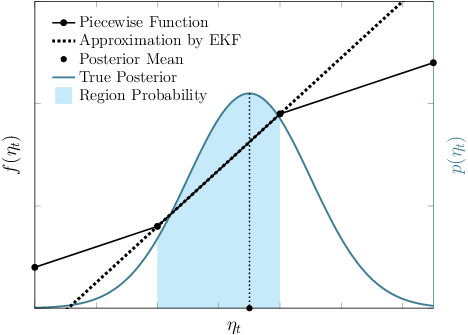
Fig. 1: A piecewise affine function f⁡(ηt)f(\eta_{t}) is locally approximated by a single line in EKF, while the proposed filter computes the first two moments of the posterior over the entire support.

Most of studies in the literature on Bayesian filtering of stochastic hybrid systems are limited to jump Markov systems [5, 6, 7, 8, 9, 10] or the so called semi-Markov jump linear systems [11, 12, 1, 13]. However, in practice, there are systems where the jump Markov model for transitions between submodels is an approximation of the reality. For example, in the JAS 39 Gripen aircraft, the dynamic of the pitch rate in the model for the flight dynamic in the longitudinal direction has a nonlinear dependence on the angle of attack [14]. Further, this nonlinear dependence is modeled by a piecewise affine function.

The exact Bayesian filtering solution for such systems is a mixture of truncated normal distributions, where the number of mixture components grows exponentially with time. When the extended Kalman filter (EKF) is used in PWASS models, the piecewise affine function is approximated by a single line, as showed in Fig. 1. This is problematic when the state uncertainty is large compared to the sizes of the regions. In this letter, we propose a Bayesian filtering algorithm for PWASS models that uses the exact time and measurement Kalman filter updates for each submodel avoiding linearization errors. In the proposed filter the cumulative distribution function (CDF) is used to compute the posterior distribution of the state as well as the probability of each region (shaded area in Fig. 1). The mixture explosion is avoided through approximating each posterior mixture of truncated normal distributions by a single normal distribution with matched moments.

II Problem formulation

Consider the PWASS model [15]

𝐱t+1=\displaystyle\mathbf{x}_{t+1}=\ ℱ⁡(𝐱t)+B​𝐮t+𝝎t,\displaystyle\mathcal{F}(\mathbf{x}_{t})+B\mathbf{u}_{t}+\boldsymbol{\omega}_{t}, (1a)
𝐲t=\displaystyle\mathbf{y}_{t}=\ C​𝐱t+𝝂t,\displaystyle C\mathbf{x}_{t}+\boldsymbol{\nu}_{t}, (1b)

where 𝐲t∈ℝny\mathbf{y}_{t}\in\mathbb{R}^{n_{y}} is the measurement; C∈ℝny×nxC\in\mathbb{R}^{n_{y}\times n_{x}} is the measurement matrix; 𝐮t∈ℝnu\mathbf{u}_{t}\in\mathbb{R}^{n_{u}} is the deterministic input; B∈ℝnx×nuB\in\mathbb{R}^{n_{x}\times n_{u}} is the input matrix; 𝝎t∈ℝnx\boldsymbol{\omega}_{t}\in\mathbb{R}^{n_{x}} and 𝝂t∈ℝny\boldsymbol{\nu}_{t}\in\mathbb{R}^{n_{y}} are the process and measurement noise terms respectively; 𝐱t∈ℝnx\mathbf{x}_{t}\in\mathbb{R}^{n_{x}} is the state vector partitioned by two scalar variables ηt\eta_{t} and ζt\zeta_{t} as well as a vector 𝝌t∈ℝ(nx−2)\boldsymbol{\chi}_{t}\in\mathbb{R}^{(n_{x}-2)} as in 𝐱t≜[ηt,ζt,𝝌tT]T\mathbf{x}_{t}\triangleq\begin{bmatrix}\eta_{t},\zeta_{t},\boldsymbol{\chi}_{t}^{\mathrm{T}}\end{bmatrix}^{\mathrm{T}}. The nonlinear function ℱ⁡(⋅)\mathcal{F}(\cdot) is the state transition function with the following structure

ℱ⁡(𝐱t)≜[ΦT​𝐱tf⁡(ηt)+ϕT​𝐳tF​𝐱t],\displaystyle\mathcal{F}(\mathbf{x}_{t})\triangleq\begin{bmatrix}\Phi^{\mathrm{T}}\mathbf{x}_{t}\\ f(\eta_{t})+\boldsymbol{\phi}^{\mathrm{T}}\mathbf{z}_{t}\\ F\mathbf{x}_{t}\end{bmatrix}, (2)

where 𝐳t≜[ζt,𝝌tT]T\mathbf{z}_{t}\triangleq\begin{bmatrix}\zeta_{t},\boldsymbol{\chi}_{t}^{\mathrm{T}}\end{bmatrix}^{\mathrm{T}}, ϕ∈ℝ(nx−1)\boldsymbol{\phi}\in\mathbb{R}^{(n_{x}-1)}, Φ∈ℝnx\Phi\in\mathbb{R}^{n_{x}}, F∈ℝ(nx−2)×nxF\in\mathbb{R}^{(n_{x}-2)\times n_{x}}; and the piecewise affine function f⁡(ηt)f(\eta_{t}) is given by

f⁡(ηt)={f1=a1​ηt+b1if ​l1<ηt≤l2⋮fNr=aNr​ηt+bNrif ​lNr<ηt<lNr+1,f(\eta_{t})=\begin{cases}f_{1}=a_{1}{\eta}_{t}+b_{1}&\text{if }{l}_{1}<{\eta}_{t}\leq{l}_{2}\\ \quad\vdots&\\ f_{N_{r}}=a_{N_{r}}{\eta}_{t}+b_{N_{r}}&\text{if }{l}_{{N_{r}}}<{\eta}_{t}<{l}_{{N_{r+1}}},\\ \end{cases} (3)

with l1=−∞l_{1}=-\infty and lNr+1=+∞l_{N_{r}+1}=+\infty. For a given region ℛi≜{𝐱t:li<ηt≤li+1}\mathcal{R}_{i}\triangleq\left\{\mathbf{x}_{t}:{l}_{i}<{\eta}_{t}\leq{l}_{i+1}\right\} it is possible to rewrite (2) using (3) as

ℱ⁡(𝐱t)\displaystyle\mathcal{F}(\mathbf{x}_{t}) =[ΦT​𝐱tai​ηt+bi+ϕT​𝐳tF​𝐱t]\displaystyle=\begin{bmatrix}\Phi^{\mathrm{T}}\mathbf{x}_{t}\\ a_{i}{\eta}_{t}+b_{i}+\boldsymbol{\phi}^{\mathrm{T}}\mathbf{z}_{t}\\ F\mathbf{x}_{t}\end{bmatrix} (4)
=[ΦT[ai​ϕT]F]⏞Ai​𝐱t+[𝟎bi𝟎]⏞𝐛i\displaystyle=\overbrace{\begin{bmatrix}\Phi^{\mathrm{T}}\\ [a_{i}~\boldsymbol{\phi}^{\mathrm{T}}]\\ F\end{bmatrix}}^{A_{i}}\mathbf{x}_{t}+\overbrace{\begin{bmatrix}\mathbf{0}\\ b_{i}\\ \mathbf{0}\end{bmatrix}}^{\mathbf{b}_{i}} (5)
=Ai​𝐱t+𝐛i.\displaystyle=A_{i}\mathbf{x}_{t}+\mathbf{b}_{i}. (6)

Hence, for a given region ℛi\mathcal{R}_{i}, the model (1) can be written as the conditionally affine state-space model

𝐱t+1=\displaystyle\mathbf{x}_{t+1}=\ Ai​𝐱t+B​𝐮t+𝐛i+𝝎t,\displaystyle A_{i}\mathbf{x}_{t}+B\mathbf{u}_{t}+\mathbf{b}_{i}+\boldsymbol{\omega}_{t}, (7a)
𝐲t=\displaystyle\mathbf{y}_{t}=\ C​𝐱t+𝝂t,\displaystyle C\mathbf{x}_{t}+\boldsymbol{\nu}_{t}, (7b)

where AiA_{i} and 𝐛i\mathbf{b}_{i} are defined in (5). The index i∈{1,⋯,Nr}i\in\left\{1,\cdots,N_{r}\right\} determines in which piecewise affine dynamics the system is at time tt, i.e., which submodel is active at time tt. The initial state has a prior distribution 𝐱1∼𝒩⁡(𝐱^1|0,P1|0)\mathbf{\mathbf{x}}_{1}\sim\mathcal{N}(\hat{\mathbf{x}}_{1|0},P_{1|0}), where 𝒩⁡(𝝁,Σ)\mathcal{N}(\boldsymbol{\mu},\Sigma) denotes a Gaussian distribution with mean 𝝁\boldsymbol{\mu} and covariance Σ\Sigma, and the subscript “t1|t2t_{1}|t_{2}” is read “at time t1t_{1} using measurements up to time t2t_{2}”. Also, we assume {𝝎t∈ℝnx|1≤t≤T}\{\boldsymbol{\omega}_{t}\in\mathbb{R}^{n_{x}}|1\leq t\leq T\} and {𝝂t∈ℝny|1≤t≤T}\{\boldsymbol{\nu}_{t}\in\mathbb{R}^{n_{y}}|1\leq t\leq T\} are mutually independent white Gaussian noise sequences with covariance QQ and RR respectively. In this letter, we propose a filter to estimate p(𝐱t|𝐲1:t)p(\mathbf{x}_{t}|\mathbf{y}_{1:t}).

III Proposed Solution

Assume that at time tt the following filtering posterior distribution for 𝐱t\mathbf{x}_{t} is available

p(𝐱t|𝐲1:t)=𝒩(𝐱t;𝐱^t|t,Pt|t).\displaystyle p(\mathbf{x}_{t}|\mathbf{y}_{1:t})=\mathcal{N}(\mathbf{x}_{t};\widehat{\mathbf{x}}_{t|t},P_{t|t}). (8)

This distribution can be rewritten using the indicator function as in

p(𝐱t|𝐲1:t)=∑i=1Nr𝟏ℛi(𝐱t)𝒩(𝐱t;𝐱^t|t,Pt|t),\displaystyle p(\mathbf{x}_{t}|\mathbf{y}_{1:t})=\sum_{i=1}^{N_{r}}\mathbf{1}_{\mathcal{R}_{i}}(\mathbf{x}_{t})\mathcal{N}(\mathbf{x}_{t};\widehat{\mathbf{x}}_{t|t},P_{t|t}), (9)

where

𝟏𝒜​(𝐱)≜{1if ​𝐱∈𝒜,0if ​𝐱∉𝒜.\displaystyle\mathbf{1}_{\mathcal{A}}(\mathbf{x})\triangleq\begin{cases}1&\text{if }\mathbf{x}\in\mathcal{A},\\ 0&\text{if }\mathbf{x}\notin\mathcal{A}.\end{cases} (10)

Using (7), the state transition density p⁡(𝐱t+1|𝐱t)p(\mathbf{x}_{t+1}|\mathbf{x}_{t}) and the likelihood function p⁡(𝐲t+1|𝐱t+1)p(\mathbf{y}_{t+1}|\mathbf{x}_{t+1}) can be written as

p⁡(𝐱t+1|𝐱t)\displaystyle p(\mathbf{x}_{t+1}|\mathbf{x}_{t}) =𝒩⁡(𝐱t+1,Ai​𝐱t+B​𝐮t+𝐛i,Q),\displaystyle=\mathcal{N}(\mathbf{x}_{t+1};A_{i}\mathbf{x}_{t}+B\mathbf{u}_{t}+\mathbf{b}_{i},Q), (11)
p⁡(𝐲t+1|𝐱t+1)\displaystyle p(\mathbf{y}_{t+1}|\mathbf{x}_{t+1}) =𝒩⁡(𝐲t+1,C​𝐱t+1,R).\displaystyle=\mathcal{N}(\mathbf{y}_{t+1};C\mathbf{x}_{t+1},R). (12)

Therefore, the joint posterior p(𝐱t,𝐱t+1,𝐲t+1|𝐲1:t)p(\mathbf{x}_{t},\mathbf{x}_{t+1},\mathbf{y}_{t+1}|\mathbf{y}_{1:t}) can be written as

p(𝐱t,𝐱t+1,𝐲t+1|𝐲1:t)=∑i=1Nr𝟏ℛi(𝐱t)𝒩(𝐱t;𝐱^t|t,Pt|t)\displaystyle p(\mathbf{x}_{t},\mathbf{x}_{t+1},\mathbf{y}_{t+1}|\mathbf{y}_{1:t})=\sum_{i=1}^{N_{r}}\mathbf{1}_{\mathcal{R}_{i}}(\mathbf{x}_{t})\mathcal{N}(\mathbf{x}_{t};\widehat{\mathbf{x}}_{t|t},P_{t|t})
×𝒩⁡(𝐱t+1,Ai​𝐱t+B​𝐮t+𝐛i,Q)​𝒩​(𝐲t+1,C​𝐱t+1,R),\displaystyle\times\mathcal{N}(\mathbf{x}_{t+1};A_{i}\mathbf{x}_{t}+B\mathbf{u}_{t}+\mathbf{b}_{i},Q)\mathcal{N}(\mathbf{y}_{t+1};C\mathbf{x}_{t+1},R), (13)

which can be rewritten in matrix form as

p⁡(CLOSE\displaystyle p( 𝐱t,𝐱t+1,𝐲t+1|𝐲1:t)\displaystyle\mathbf{x}_{t},\mathbf{x}_{t+1},\mathbf{y}_{t+1}|\mathbf{y}_{1:t})
=∑i=1Nr𝟏ℛi​(𝐱t)​𝒩​([𝐱tT,𝐱t+1T,𝐲t+1T]T,𝝁t,i,Σt,i),\displaystyle=\sum_{i=1}^{N_{r}}\mathbf{1}_{\mathcal{R}_{i}}(\mathbf{x}_{t})\mathcal{N}([\mathbf{x}_{t}^{\mathrm{T}},\mathbf{x}_{t+1}^{\mathrm{T}},\mathbf{y}_{t+1}^{\mathrm{T}}]^{\mathrm{T}};\boldsymbol{\mu}_{t,i},\Sigma_{t,i}), (14)

where

𝝁t,i=Δ[𝝁1​i𝝁2​i]=\displaystyle\boldsymbol{\mu}_{t,i}\stackrel{{\scriptstyle\Delta}}{{=}}\left[\begin{array}[]{c}\hbox{\multirowsetup$\boldsymbol{\mu}_{1i}$}\\ \\ \hline\cr\boldsymbol{\mu}_{2i}\end{array}\right]= [𝐱^t|tAi​𝐱^t|t+B​𝐮t+𝐛iC​Ai​𝐱^t|t+C⁡(B​𝐮t+𝐛i)]\displaystyle\left[\begin{array}[]{c}\widehat{\mathbf{x}}_{t|t}\\ A_{i}\widehat{\mathbf{x}}_{t|t}+B\mathbf{u}_{t}+\mathbf{b}_{i}\\ \hline\cr CA_{i}\widehat{\mathbf{x}}_{t|t}+C(B\mathbf{u}_{t}+\mathbf{b}_{i})\end{array}\right]

and

Σt,i≜[Σ11​iΣ12​iΣ21​iΣ22​i]=\displaystyle\Sigma_{t,i}\triangleq\left[\begin{array}[]{c|c}\Sigma_{11i}&\Sigma_{12i}\\ \hline\cr\Sigma_{21i}&\Sigma_{22i}\end{array}\right]=
[Pt|tPt|t​AiT(Pt|t​AiT)​CTAi​Pt|tAi​Pt|t​AiT+Q(Ai​Pt|t​AiT+Q)T​CTC⁡(Ai​Pt|t)C⁡(Ai​Pt|t​AiT+Q)C⁡(Ai​Pt|t​AiT+Q)​CT+R].\displaystyle\left[\begin{array}[]{cc|c}P_{t|t}&P_{t|t}A_{i}^{\mathrm{T}}&(P_{t|t}A_{i}^{T})C^{T}\\ A_{i}P_{t|t}&A_{i}P_{t|t}A_{i}^{\mathrm{T}}+Q&(A_{i}P_{t|t}A_{i}^{\mathrm{T}}+Q)^{T}C^{T}\\ \hline\cr C(A_{i}P_{t|t})&C(A_{i}P_{t|t}A_{i}^{\mathrm{T}}+Q)&C(A_{i}P_{t|t}A_{i}^{\mathrm{T}}+Q)C^{\mathrm{T}}+R\\ \end{array}\right].

The conditional distribution of 𝐱t\mathbf{x}_{t} and 𝐱t+1\mathbf{x}_{t+1} given 𝐲t+1\mathbf{y}_{t+1} is

p\displaystyle p (𝐱t,𝐱t+1|𝐲1:t+1)=1Ztp(𝐱t,𝐱t+1,𝐲t+1|𝐲1:t)\displaystyle(\mathbf{x}_{t},\mathbf{x}_{t+1}|\mathbf{y}_{1:t+1})=\frac{1}{Z_{t}}p(\mathbf{x}_{t},\mathbf{x}_{t+1},\mathbf{y}_{t+1}|\mathbf{y}_{1:t}) (26)
=1Zt​∑i=1Nr𝟏ℛi​(𝐱t)​𝒩​([𝐱tT,𝐱t+1T,𝐲t+1T]T,𝝁t,i,Σt,i)\displaystyle=\frac{1}{Z_{t}}\sum_{i=1}^{N_{r}}\mathbf{1}_{\mathcal{R}_{i}}(\mathbf{x}_{t})\mathcal{N}([\mathbf{x}_{t}^{\mathrm{T}},\mathbf{x}_{t+1}^{\mathrm{T}},\mathbf{y}_{t+1}^{\mathrm{T}}]^{\mathrm{T}};\boldsymbol{\mu}_{t,i},\Sigma_{t,i}) (27)
=1Zt​∑i=1Nr𝟏ℛi​(𝐱t)​𝒩​(𝐲t+1,𝝁2​i,Σ22​i)\displaystyle=\frac{1}{Z_{t}}\sum_{i=1}^{N_{r}}\mathbf{1}_{\mathcal{R}_{i}}(\mathbf{x}_{t})\mathcal{N}(\mathbf{y}_{t+1};\boldsymbol{\mu}_{2i},\Sigma_{22i})
×𝒩⁡([𝐱tT,𝐱t+1T]T,𝝁~i,Σ~i),\displaystyle\hskip 85.35826pt\times\mathcal{N}([\mathbf{x}_{t}^{\mathrm{T}},\mathbf{x}_{t+1}^{\mathrm{T}}]^{\mathrm{T}};\tilde{\boldsymbol{\mu}}_{i},\tilde{\Sigma}_{i}), (28)

where

𝝁~i\displaystyle\tilde{\boldsymbol{\mu}}_{i} =Δ[𝝁~1​i𝝁~2​i]=𝝁1​i+Σ21​iT​Σ22​i−1​(𝐲t+1−𝝁2​i),\displaystyle\stackrel{{\scriptstyle\Delta}}{{=}}\left[\begin{array}[]{c}\tilde{\boldsymbol{\mu}}_{1i}\\ \hline\cr\tilde{\boldsymbol{\mu}}_{2i}\end{array}\right]=\boldsymbol{\mu}_{1i}+\Sigma_{21i}^{T}\Sigma_{22i}^{-1}(\mathbf{y}_{t+1}-\boldsymbol{\mu}_{2i}),
Σ~i\displaystyle\tilde{\Sigma}_{i} =Δ[Σ~11​iΣ~12​iΣ~21​iΣ~22​i]=Σ11​i−Σ21​iT​Σ22​i−1​Σ21​i,\displaystyle\stackrel{{\scriptstyle\Delta}}{{=}}\left[\begin{array}[]{c|c}\tilde{\Sigma}_{11i}&\tilde{\Sigma}_{12i}\\ \hline\cr\tilde{\Sigma}_{21i}&\tilde{\Sigma}_{22i}\end{array}\right]=\Sigma_{11i}-\Sigma_{21i}^{T}\Sigma_{22i}^{-1}\Sigma_{21i},

ZtZ_{t} is a normalizing constant, and the partitions in (III) and (III) have equal dimensions. The quantities Pr(𝐱t∈ℛi|𝐲1:t+1)\Pr(\mathbf{x}_{t}\in\mathcal{R}_{i}|\mathbf{y}_{1:t+1}) for i=1⋯Nri=1\cdots N_{r} as well as the normalizing constant ZtZ_{t} can be computed via integration of p(𝐱t,𝐱t+1|𝐲1:t+1)p(\mathbf{x}_{t},\mathbf{x}_{t+1}|\mathbf{y}_{1:t+1}) as in

Pr(𝐱t∈ℛi|𝐲1:t+1)\displaystyle\Pr(\mathbf{x}_{t}\in\mathcal{R}_{i}|\mathbf{y}_{1:t+1})
=1Zt​𝒩​(𝐲t+1,𝝁2​i,Σ22​i)​∫ℛi𝒩⁡(𝐱t,𝝁~1​i,Σ~11​i)​d​𝐱t\displaystyle=\frac{1}{Z_{t}}\mathcal{N}(\mathbf{y}_{t+1};\boldsymbol{\mu}_{2i},\Sigma_{22i})\int_{\mathcal{R}_{i}}\mathcal{N}(\mathbf{x}_{t};\tilde{\boldsymbol{\mu}}_{1i},\tilde{\Sigma}_{11i})\;\mathrm{d}\mathbf{x}_{t} (33)
=1Zt​𝒩​(𝐲t+1,𝝁2​i,Σ22​i)​Γi,\displaystyle=\frac{1}{Z_{t}}\mathcal{N}(\mathbf{y}_{t+1};\boldsymbol{\mu}_{2i},\Sigma_{22i})\;\Gamma_{i}, (34)

where

Γi=Δ∫li<ηt≤li+1𝒩⁡(ηt,[𝝁~1​i](1,1),[Σ~11​i](1,1))​d​ηt\displaystyle\Gamma_{i}\stackrel{{\scriptstyle\Delta}}{{=}}\int_{{l}_{i}<{\eta}_{t}\leq{l}_{i+1}}\mathcal{N}(\eta_{t};[\tilde{\boldsymbol{\mu}}_{1i}]_{(1,1)},[\tilde{\Sigma}_{11i}]_{(1,1)})\;\mathrm{d}\eta_{t} (35)
=12​erf​(li+1−[𝝁~1​i](1,1)2​[Σ~11​i](1,1))−12​erf​(li−[𝝁~1​i](1,1)2​[Σ~11​i](1,1)),\displaystyle=\frac{1}{2}\text{erf}\left(\frac{l_{i+1}-[\tilde{\boldsymbol{\mu}}_{1i}]_{(1,1)}}{\sqrt{2[\tilde{\Sigma}_{11i}]_{(1,1)}}}\right)-\frac{1}{2}\text{erf}\left(\frac{l_{i}-[\tilde{\boldsymbol{\mu}}_{1i}]_{(1,1)}}{\sqrt{2[\tilde{\Sigma}_{11i}]_{(1,1)}}}\right), (36)

where the erf​(⋅)\text{erf}(\cdot) is the error function, [Σ](i,j)[\Sigma]_{(i,j)} is the element in row ii and column jj of Σ\Sigma, and

Zt=∑i=1NrN⁡(𝐲t+1,𝝁2​i,Σ22​i)​Γi.{Z_{t}}=\sum_{i=1}^{N_{r}}N(\mathbf{y}_{t+1};\boldsymbol{\mu}_{2i},\Sigma_{22i})\;\Gamma_{i}. (37)

The probability Pr(𝐱t∈ℛi|𝐲1:t+1)\Pr(\mathbf{x}_{t}\in\mathcal{R}_{i}|\mathbf{y}_{1:t+1}) represents the probability that the state be in the region ℛi\mathcal{R}_{i} at time tt given all information up to time t+1t+1. The filtering posterior distribution p(𝐱t+1|𝐲1:t+1)p(\mathbf{x}_{t+1}|\mathbf{y}_{1:t+1}) can be computed via the integration

p(𝐱t+1|𝐲1:t+1)=1Zt∫p(𝐱t,𝐱t+1,𝐲t+1|𝐲1:t)d𝐱t\displaystyle p(\mathbf{x}_{t+1}|\mathbf{y}_{1:t+1})=\frac{1}{Z_{t}}\int{p(\mathbf{x}_{t},\mathbf{x}_{t+1},\mathbf{y}_{t+1}|\mathbf{y}_{1:t})\;\mathrm{d}\mathbf{x}_{t}} (38)
=1Zt​∑i=1Nr𝒩⁡(𝐲t+1,𝝁2​i,Σ22​i)\displaystyle=\frac{1}{Z_{t}}\sum_{i=1}^{N_{r}}\mathcal{N}(\mathbf{y}_{t+1};\boldsymbol{\mu}_{2i},\Sigma_{22i})
×∫ℛi𝟏ℛi​(𝐱t)​𝒩​([𝐱tT,𝐱t+1T]T,𝝁~i,Σ~i)​d​𝐱t.\displaystyle\hskip 28.45274pt\times\int_{\mathcal{R}_{i}}\mathbf{1}_{\mathcal{R}_{i}}(\mathbf{x}_{t})\mathcal{N}([\mathbf{x}_{t}^{\mathrm{T}},\mathbf{x}_{t+1}^{\mathrm{T}}]^{\mathrm{T}};\tilde{\boldsymbol{\mu}}_{i},\tilde{\Sigma}_{i})\;\mathrm{d}\mathbf{x}_{t}. (39)

The joint posterior distribution on the right-hand side of (39) is a mixture of doubly truncated multivariate normal distributions (DTMND) [16]. In order to have a recursive algorithm, the posterior will be approximated by a normal distribution. To this end, the mean and the covariance of the posterior distribution p(𝐱t+1|𝐲1:t+1)p(\mathbf{x}_{t+1}|\mathbf{y}_{1:t+1}) is needed. The mean and covariance of a mixture distribution can be computed using the mean and the covariance of the components of the mixture density via standard moment matching formulas [17]. Hence, the problem boils down to computing the mean and the covariance of the DTMND which is presented in the Apendix A.

The proposed filter for PWASS models will be referred to by PAKF (Piecewise Affine Kalman Filter). The filtering recursion is given in TABLE I. The expressions for computing the mean and the covariance of a DTMND for a given region ℛi\mathcal{R}_{i} are given in the lines 1818 and 1919 of TABLE I. The probabilities Pr(𝐱t∈ℛi|𝐲1:t+1)\Pr(\mathbf{x}_{t}\in\mathcal{R}_{i}|\mathbf{y}_{1:t+1}) as well as the normalizing constant ZtZ_{t} are calculated in the lines 21 and 22 and are used within the moment matching whose formulas are given in the lines 2323 and 2424 of TABLE I.

TABLE I: Filtering recursion for PWASS models using the Piecewise Affine Kalman Filter (PAKF)
 
1: Inputs: Ai,𝐛i,li,i=1​…,NrA_{i},\mathbf{b}_{i},l_{i},~i=1\dots,N_{r}, BB, CC, QQ, RR, 𝐮t\mathbf{u}_{t}, 𝐲t+1,𝐱^t|t,Pt|t\mathbf{y}_{t+1},\widehat{\mathbf{x}}_{t|t},P_{t|t}
2: for ii = 1 to NrN_{r} do
3: Kalman filter prediction step
4:    𝝁1​i←[𝐱^t|tAi​𝐱^t|t+B​𝐮t+𝐛i]\boldsymbol{\mu}_{1i}\leftarrow\left[\begin{smallmatrix}\widehat{\mathbf{x}}_{t|t}\\ A_{i}\widehat{\mathbf{x}}_{t|t}+B\mathbf{u}_{t}+\mathbf{b}_{i}\end{smallmatrix}\right]
5:    𝝁2​i←C​Ai​𝐱^t|t+C⁡(B​𝐮t+𝐛i)\boldsymbol{\mu}_{2i}\leftarrow CA_{i}\widehat{\mathbf{x}}_{t|t}+C(B\mathbf{u}_{t}+\mathbf{b}_{i})
6:    Σ11​i←[Pt|tPt|t​AiTAi​Pt|tAi​Pt|t​AiT+Q]\Sigma_{11i}\leftarrow\left[\begin{smallmatrix}P_{t|t}&P_{t|t}A_{i}^{\mathrm{T}}\\ A_{i}P_{t|t}&A_{i}P_{t|t}A_{i}^{\mathrm{T}}+Q\\ \end{smallmatrix}\right]
7:    Σ22​i←C⁡(Ai​Pt|t​AiT+Q)​CT+R\Sigma_{22i}\leftarrow C(A_{i}P_{t|t}A_{i}^{\mathrm{T}}+Q)C^{\mathrm{T}}+R
8:    Σ21​i←[C⁡(Ai​Pt|t)C⁡(Ai​Pt|t​AiT+Q)]\Sigma_{21i}\leftarrow\left[\begin{smallmatrix}C(A_{i}P_{t|t})&C(A_{i}P_{t|t}A_{i}^{\mathrm{T}}+Q)\end{smallmatrix}\right]
9: Kalman filter update step
10:    𝝁~i←𝝁1​i+Σ21​iT​Σ22​i−1​(yt+1−𝝁2​i)\tilde{\boldsymbol{\mu}}_{i}\leftarrow\boldsymbol{\mu}_{1i}+\Sigma_{21i}^{T}\Sigma_{22i}^{-1}(y_{t+1}-\boldsymbol{\mu}_{2i})
11:    Σ~i←Σ11​i−Σ21​iT​Σ22​i−1​Σ21​i\tilde{\Sigma}_{i}\leftarrow\Sigma_{11i}-\Sigma_{21i}^{T}\Sigma_{22i}^{-1}\Sigma_{21i}
12: Computing integral (34)
13:    wi←12​erf​(li+1−[𝝁~1​i](1,1)2​[Σ~11​i](1,1))−12​erf​(li−[𝝁~1​i](1,1)2​[Σ~11​i](1,1))w_{i}\leftarrow\frac{1}{2}\text{erf}\left(\frac{l_{i+1}-[\tilde{\boldsymbol{\mu}}_{1i}]_{(1,1)}}{\sqrt{2[\tilde{\Sigma}_{11i}]_{(1,1)}}}\right)-\frac{1}{2}\text{erf}\left(\frac{l_{i}-[\tilde{\boldsymbol{\mu}}_{1i}]_{(1,1)}}{\sqrt{2[\tilde{\Sigma}_{11i}]_{(1,1)}}}\right)
14:    wi←𝒩⁡(𝐲t+1,𝝁2​i,Σ22​i)×wiw_{i}\leftarrow\mathcal{N}(\mathbf{y}_{t+1};\boldsymbol{\mu}_{2i},\Sigma_{22i})\times w_{i}
15: Computing mean and covariance of the DTMND
16:   Λ←chol(Σ~i,′lower′)\Lambda\leftarrow\mathrm{chol}(\tilde{\Sigma}_{i},^{\prime}lower^{\prime}) ⊳\triangleright (Cholesky decomposition)
17:   λ1←li−[𝝁~i](1,1)[Λ](1,1)\lambda_{1}\leftarrow\frac{l_{i}-[\tilde{\boldsymbol{\mu}}_{i}]_{(1,1)}}{[\Lambda]_{(1,1)}}
18:   λ2←li+1−[𝝁~i](1,1)[Λ](1,1)\lambda_{2}\leftarrow\frac{l_{i+1}-[\tilde{\boldsymbol{\mu}}_{i}]_{(1,1)}}{[\Lambda]_{(1,1)}}
19:   𝒵←12​erf​(λ22)−12​erf​(λ12)\mathcal{Z}\leftarrow\frac{1}{2}\text{erf}\left(\frac{\lambda_{2}}{\sqrt{2}}\right)-\frac{1}{2}\text{erf}\left(\frac{\lambda_{1}}{\sqrt{2}}\right)
20:   mi​1←𝒩⁡(λ1,0,1)−𝒩⁡(λ2,0,1)𝒵m_{i1}\leftarrow\frac{\mathcal{N}(\lambda_{1};0,1)-\mathcal{N}(\lambda_{2};0,1)}{\mathcal{Z}}
21:   si​1←1+λ1​𝒩​(λ1,0,1)−λ2​𝒩​(λ2,0,1)𝒵−(mi​1)2s_{i1}\leftarrow 1+\frac{\lambda_{1}\mathcal{N}(\lambda_{1};0,1)-\lambda_{2}\mathcal{N}(\lambda_{2};0,1)}{\mathcal{Z}}-({m}_{i1})^{2}
22:   𝐦i←Λ⁡[mi​1𝟎2​nx−1]+𝝁~i\mathbf{m}_{i}\leftarrow\Lambda\left[\begin{smallmatrix}m_{i1}\\ \mathbf{0}_{2n_{x}-1}\end{smallmatrix}\right]+\tilde{\boldsymbol{\mu}}_{i}
23:   Si←Λ⁡[si​1𝟎2​nx−1T𝟎2​nx−1I2​nx−1]​ΛTS_{i}\leftarrow\Lambda\left[\begin{smallmatrix}s_{i1}&\mathbf{0}_{2n_{x}-1}^{\mathrm{T}}\\ \mathbf{0}_{2n_{x}-1}&I_{2n_{x}-1}\end{smallmatrix}\right]\Lambda^{\mathrm{T}}
24: end for
25: Normalizing constant (37)
26: Zt←∑i=1NrwiZ_{t}\leftarrow{\sum_{i=1}^{N_{r}}w_{i}}
27: wi←wiZtw_{i}\leftarrow\frac{w_{i}}{Z_{t}}
28: Moment matching
29: 𝐦^t←∑i=1Nrwi​𝐦i\widehat{\mathbf{m}}_{t}\leftarrow\sum_{i=1}^{N_{r}}w_{i}~\mathbf{m}_{i}
30: Pt←∑i=1Nrwi​(Si+(𝐦i−𝐦^t)​(𝐦i−𝐦^t)T)P_{t}\leftarrow\sum_{i=1}^{N_{r}}w_{i}\left(S_{i}+(\mathbf{m}_{i}-\widehat{\mathbf{m}}_{t})(\mathbf{m}_{i}-\widehat{\mathbf{m}}_{t})^{\mathrm{T}}\right)
31: 𝐱^t+1|t+1←[𝐦^t]nx+1:2​nx\widehat{\mathbf{x}}_{t+1|t+1}\leftarrow[\widehat{\mathbf{m}}_{t}]_{n_{x}+1:2n_{x}}
32: Pt+1|t+1←[Pt]nx+1:2​nx,nx+1:2​nxP_{t+1|t+1}\leftarrow[P_{t}]_{n_{x}+1:2n_{x},n_{x}+1:2n_{x}}
33: Outputs: 𝐱^t+1|t+1\widehat{\mathbf{x}}_{t+1|t+1} and Pt+1|t+1P_{t+1|t+1}
 

IV Numerical Simulations

Numerical simulations are performed to evaluate the performance of PAKF. In these simulations, PAKF is compared to the extended Kalman filter (EKF) and the marginalized particle filter (MPF) [18, 19]. The EKF expressions for PWASS models are those in the lines 3​-​93\text{-}9 of TABLE I. In EKF, they are evaluated only for the region where 𝐱^t|t\widehat{\mathbf{x}}_{t|t} is located at time tt. The MPF is used to compute the optimal Bayesian solution. This optimal solution will be used as a reference in the evaluation of PAKF. All numerical computations are done using MATLAB.

TABLE II: Parameters of the SDOFS model
Param. Δ​t\Delta t (s) DD (N⋅\cdots/mm) MM (t) aa (N/mm) l1,l2l_{1},l_{2} (mm)
Value 0.01 1 1 [50​5​50][50~5~50] 11

Nonlinear vibrations caused by clearance can be modeled as a single-degree-of-freedom system (SDOFS) with piecewise affine spring characteristics [20]. Fig. 2 shows the physical model of SDOFS and Fig. 3 presents its piecewise affine spring characteristic. The discretized PWASS model for the SDOFS can be written as

𝐱t+1\displaystyle\mathbf{x}_{t+1} =Δ[ηt+1ζt+1]=[1Δ​t−Δ​t​aiM1−Δ​t​DM]​𝐱t\displaystyle\stackrel{{\scriptstyle\Delta}}{{=}}\begin{bmatrix}\eta_{t+1}\\ \zeta_{t+1}\end{bmatrix}=\begin{bmatrix}1&\Delta t\\ -\frac{\Delta ta_{i}}{M}&1-\frac{\Delta tD}{M}\end{bmatrix}\mathbf{x}_{t}
+[0Δ​tM]​𝐮t+[0−Δ​t​biM]+𝝎t,\displaystyle\hskip 48.36958pt+\begin{bmatrix}0\\ \frac{\Delta t}{M}\end{bmatrix}\mathbf{u}_{t}+\begin{bmatrix}0\\ -\frac{\Delta tb_{i}}{M}\end{bmatrix}+\boldsymbol{\omega}_{t}, (40a)
𝐲t\displaystyle\mathbf{y}_{t} =[10]​𝐱t+𝝂t,\displaystyle=\begin{bmatrix}1&0\end{bmatrix}\mathbf{x}_{t}+\boldsymbol{\nu}_{t}, (40b)

where ηt\eta_{t} and ζt\zeta_{t} are the position in [mm] and the velocity in [mm/s] of the mass MM, respectively, Δ​t\Delta t is the sampling time, DD is the damping coefficient, and aia_{i} and bib_{i} are the piecewise affine spring coefficients such that

f⁡(ηt)={f1=a1​ηt+b1if −∞<ηt≤l1f2=a2​ηt+b2if l1<ηt≤l2f3=a3​ηt+b3if l2<ηt<+∞f(\eta_{t})=\begin{cases}f_{1}=a_{1}{\eta}_{t}+b_{1}&\text{if }-\infty<{\eta}_{t}\leq{l}_{1}\\ f_{2}=a_{2}{\eta}_{t}+b_{2}&\text{if }\quad~{l}_{1}<{\eta}_{t}\leq{l}_{2}\\ f_{3}=a_{3}{\eta}_{t}+b_{3}&\text{if }\quad~l_{2}<{\eta}_{t}<+\infty\end{cases} (41)

with a3=a1,b1=l1​(a2−a1),b2=0a_{3}=a_{1},b_{1}=l_{1}(a_{2}-a_{1}),b_{2}=0 and b3=l2​(a2−a3)b_{3}=l_{2}(a_{2}-a_{3}). Monte Carlo (MC) simulations are performed, where the model (40) is simulated for T=400T=400 time steps. The parameters values are given in TABLE II. Further, 𝐱1\mathbf{\mathbf{x}}_{1} is sampled from standard bivariate normal distribution, 𝝂t∼𝒩⁡(0,1)\boldsymbol{\nu}_{t}\sim\mathcal{N}(0,1), 𝝎t∼𝒩⁡([0​0]T,diag​[0.01 0.01])\boldsymbol{\omega}_{t}\sim\mathcal{N}([0~0]^{T},\text{diag}[0.01\ 0.01]) and 𝐮t∼𝒩⁡(0,52)\mathbf{u}_{t}\sim\mathcal{N}(0,5^{2}). For the MPF, we use 10 000 particles.

We compare the three filters in terms of the root mean square error (RMSE) between the true state and the predicted state

RMSE​(𝐱(j))=12​T​∑t=1T((ηt(j)−η^t|t(j))2+(ζt(j)−ζ^t|t(j))2),\text{RMSE}({\mathbf{x}}^{(j)})=\sqrt{\frac{1}{2T}\sum_{t=1}^{T}\left((\eta_{t}^{(j)}-\hat{\eta}_{t|t}^{(j)})^{2}+(\zeta_{t}^{(j)}-\hat{\zeta}_{t|t}^{(j)})^{2}\right)}, (42)

where 𝐱^t|t(j)=[η^t|t(j)​ζ^t|t(j)]T\widehat{\mathbf{x}}_{t|t}^{(j)}=\left[\hat{\eta}_{t|t}^{(j)}~\hat{\zeta}_{t|t}^{(j)}\right]^{\mathrm{T}} and 𝐱t(j)=[ηt(j)​ζt(j)]T\mathbf{x}_{t}^{(j)}=\left[\eta_{t}^{(j)}~\zeta_{t}^{(j)}\right]^{\mathrm{T}} denote the estimated mean of the state 𝐱t\mathbf{x}_{t} and its true value in the jjth MC run, respectively. Columns two and three of Table III show the average over 5 000 MC simulations of RMSE (ARMSE) for each filter as well as the standard deviation of the RMSE (STD). We noticed that the ARMSE for PAKF is 5.35%5.35\% smaller than that of the EKF. The ARMSE for MPF is 0.12%0.12\% smaller than that of the PAKF. We also noticed that EKF has the highest STD of all the filters. The Fig. 4 presents the cumulative distribution of the RMSE for each filter. The minimum and maximum RMSE values for each filter are presented in the last two columns of TABLE III.

TABLE III: Filter comparison results.
Filter ARMSE STD min. RMSE max. RMSE
EKF 0.88327 0.30612 0.25792 2.09761
PAKF 0.83600 0.27931 0.27256 2.05709
MPF 0.83505 0.27994 0.26467 2.04196

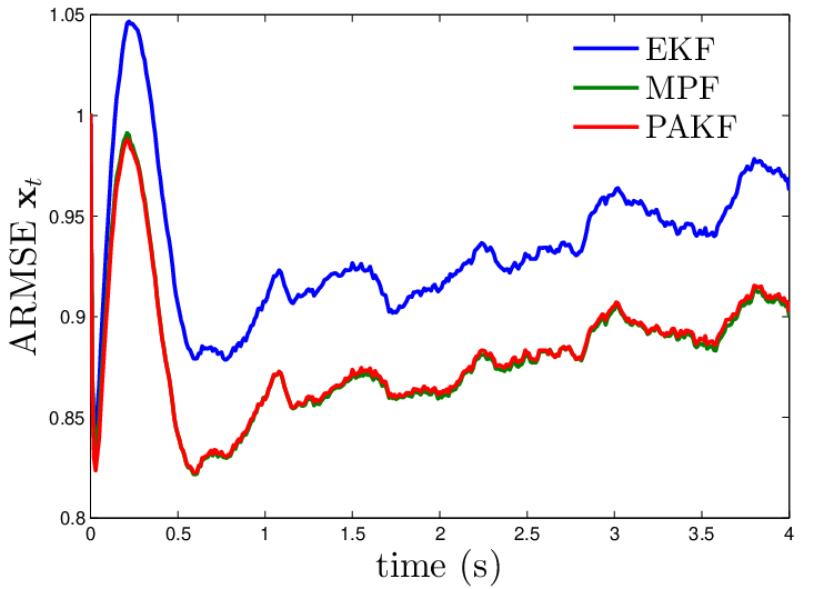
Fig. 5 shows the ARMSE between the simulated state and the estimated state as a function of time for the PAKF, MPF, and EKF. We noticed that the ARMSE for EKF is always above the ARMSE of PAKF and MPF. That is, PAKF and the MPF outperform EKF both for initial parts of the path and in the stabilized state. The MPF and PAKF have similar performance, but MPF is computationally expensive. For 10 000 particles, MPF takes six times more time to complete one MC run than PAKF.

V Conclusion

The proposed filter (PAKF) obtains estimation error close to that of the optimal filter (MPF) for a particular class of PWASS models which are discussed in this letter. The filter’s performance is tested in an example where the measurement noise variance is greater than the process noise variances and the comparison filters are EKF and MPF. The filtering recursion of PAKF involves approximation of the posterior distribution. Despite the approximations, PAKF obtains estimation error close to MPF and 5.35%5.35\% better than EKF. Furthermore, the computation time is roughly six times less than a MPF with comparable performance.

Refer to caption
Fig. 2: SDOFS physical model with piecewise affine spring characteristics.
Refer to caption
Fig. 3: Piecewise affine spring characteristics of model in Fig. 2 .
Refer to caption
Fig. 4: Cumulative distribution of the RMSE for EKF, MPF and PAKF.
Refer to caption
Fig. 5: ARMSE for EKF, MPF and PAKF as a function of time.

References

  • [1] C. E. Seah and I. Hwang, “State estimation for stochastic linear hybrid systems with continuous-state-dependent transitions: An imm approach,” IEEE Transactions on Aerospace and Electronic Systems, vol. 45, no. 1, pp. 376–392, 2009.
  • [2] A. Doucet, N. Gordon, and V. Kroshnamurthy, “Particle filters for state estimation of jump markov linear systems,” IEEE Transactions on Signal Processing, vol. 49, no. 3, pp. 613–624, mar 2001.
  • [3] R. Porreca, S. Drulhe, H. de Jong, and G. Ferrari-Trecate, “Identification of parameters and structure of piecewise affine models of genetic networks,” IFAC Proceedings Volumes, vol. 42, no. 10, pp. 587–592, 2009.
  • [4] R. Vidal and Y. Ma, “A unified algebraic approach to 2-d and 3-d motion segmentation and estimation,” Journal of Mathematical Imaging and Vision, vol. 25, no. 3, pp. 403–421, oct 2006.
  • [5] K. P. Murphy, “Learning switching kalman filter models,” Compaq Cambridge Research Lab, Tech. Rep. August, 1998.
  • [6] Z. Ghahramani and G. E. Hinton, “Variational learning for switching state-space models,” Neural Computation, vol. 12, no. 4, pp. 831–864, apr 2000.
  • [7] D. Barber, “Expectation correction for smoothed inference in switching linear dynamical systems,” Journal of Machine Learning Research, vol. 7, pp. 2515–2540, 2006.
  • [8] D. Barber and B. Mesot, “A novel gaussian sum smoother for approximate inference in switching linear dynamical systems,” in Advances in Neural Information Processing Systems 18, 2007, pp. 4–11.
  • [9] B. Mesot, “Inference in switching linear dynamical systems applied to noise robust speech recognition of isolated digits,” Ph.D. dissertation, Ecole Polytechnique Fédérale de Lausanne, 2008.
  • [10] E. Özkan, V. Šmídl, S. Saha, C. Lundquist, and F. Gustafsson, “Marginalized adaptive particle filtering for nonlinear models with unknown time-varying noise parameters,” Automatica, vol. 49, no. 6, pp. 1566–1575, jun 2013.
  • [11] I. Hwang and C. E. Seah, “An estimation algorithm for stochastic linear hybrid systems with continuous-state-dependent mode transitions,” in Proceedings of the 45th IEEE Conference on Decision and Control. IEEE, 2006, pp. 131–136.
  • [12] H. Blom and E. Bloem, “Exact bayesian and particle filtering of stochastic hybrid systems,” IEEE Transactions on Aerospace and Electronic Systems, vol. 43, no. 1, pp. 55–70, jan 2007.
  • [13] A. Capponi, “A convex optimization approach to filtering in jump linear systems with state dependent transitions,” Automatica, vol. 46, no. 2, pp. 383–389, 2010.
  • [14] R. Larsson and M. Enqvist, “Sequential aerodynamic model parameter identification,” in 16th IFAC Symposium on System Identification, K. Michel, Ed., jul 2012, pp. 1413–1418.
  • [15] G. Andrea, “A survey on switched and piecewise affine system identification,” in 16th IFAC Symposium on System Identification, K. Michel, Ed., jul 2012, pp. 344–355.
  • [16] H. Nurminen, R. Rui, T. Ardeshiri, A. Bazanella, and F. Gustafsson, “Mean and covariance matrix of a multivariate normal distribution with one doubly-truncated component,” Department of Electrical Engineering, Linköping University, SE-581 83 Linköping, Sweden, Tech. Rep. LiTH-ISY-R-3092, July 2016. [Online]. Available: http://urn.kb.se/resolve?urn=urn:nbn:se:liu:diva-130089
  • [17] A. Runnalls, “Kullback-leibler approach to gaussian mixture reduction,” IEEE Transactions on Aerospace and Electronic Systems, vol. 43, no. 3, pp. 989–999, jul 2007.
  • [18] A. Doucet, N. de Freitas, K. Murphy, and S. Russell, “Rao-blackwellised particle filtering for dynamic bayesian networks,” in Sixteenth conference on Uncertainty in artificial intelligence, 2000, pp. 176–183.
  • [19] T. Schön, F. Gustafsson, and P.-J. Nordlund, “Marginalized particle filters for mixed linear/nonlinear state-space models,” IEEE Transactions on Signal Processing, vol. 53, no. 7, pp. 2279–2289, jul 2005.
  • [20] I. Mahfouz and F. Badrakhan, “Chaotic behaviour of some piecewise-linear systems, part ii: Systems with clearance,” Journal of Sound and Vibration, vol. 143, no. 2, pp. 289–328, dec 1990.
  • [21] Å. Björck, Numerical Methods for Least Squares Problems. SIAM, 1996.
  • [22] N. L. Johnson, S. Kotz, and N. Balakrishnan, Continuous Univariate Distributions, Vol. 1, 2nd ed. John Wiley & Sons, Inc., November 1994.

Appendix A Mean and covariance matrix of DTMND

A doubly-truncated multivariate normal distribution (DTMND) is a multivariate normal distribution, where one component is truncated from both below and above. Without loss of generality, we assume that the double truncation is applied to the first component of the random vector. For numerical methods, evaluating the presented formulas requires evaluation of the Cholesky decomposition [21, Ch. 2.2.2] as well as the probability density function (PDF) and cumulative density function (CDF) of the univariate standard normal distribution.

A-A Formulas for mean and covariance matrix

Let 𝐱∈ℝn\mathbf{x}\in\mathbb{R}^{n} be a random variable of the DTMND with the PDF

p⁡(𝐱)∝𝒩⁡(𝐱,𝝁,Σ)⋅𝟏[l1,l2]​([𝐱]1),\displaystyle p(\mathbf{x})\propto\mathcal{N}(\mathbf{x};\boldsymbol{\mu},\Sigma)\cdot\mathbf{1}_{[l_{1},l_{2}]}([\mathbf{x}]_{1}), (43)

where 𝝁∈ℝn\boldsymbol{\mu}\in\mathbb{R}^{n} is the location parameter vector, Σ∈ℝn×n\Sigma\in\mathbb{R}^{n\times n} is the positive definite squared-scale matrix, and l1,l2∈ℝl_{1},l_{2}\in\mathbb{R} are the truncation limits. Further, let Λ\Lambda be the lower triangular matrix for which Σ=Λ​ΛT\Sigma=\Lambda\Lambda^{\mathrm{T}} and whose diagonal entries are strictly positive. This type of square-root matrix can be obtained using the Cholesky decomposition [21, Ch. 2.2.2].

Then, the expectation value and covariance matrix of 𝐱\mathbf{x} are

𝔼[𝐱]\displaystyle\mathop{\mathbb{E}}[\mathbf{x}] =Λ​[m∗𝟎n−1]+𝝁\displaystyle=\Lambda\begin{bmatrix}m^{\ast}\\ \mathbf{0}_{n-1}\end{bmatrix}+\boldsymbol{\mu} (44)
𝕍⁡[𝐱]\displaystyle\mathbb{V}[\mathbf{x}] =Λ​[s∗𝟎n−1T𝟎n−1In−1]​ΛT\displaystyle=\Lambda\begin{bmatrix}s^{\ast}&\mathbf{0}_{n-1}^{\mathrm{T}}\\ \mathbf{0}_{n-1}&I_{n-1}\end{bmatrix}\Lambda^{\mathrm{T}} (45)

where

m∗\displaystyle m^{\ast} =ϕ⁡(λ1)−ϕ⁡(λ2)𝒵,\displaystyle=\frac{\phi(\lambda_{1})-\phi(\lambda_{2})}{\mathcal{Z}}, (46)
s∗\displaystyle s^{\ast} =1+λ1​ϕ​(λ1)−λ2​ϕ​(λ2)𝒵−(m∗)2,\displaystyle=1+\frac{\lambda_{1}\phi(\lambda_{1})-\lambda_{2}\phi(\lambda_{2})}{\mathcal{Z}}-(m^{\ast})^{2}, (47)

with

λ1=l1−[𝝁]1[Λ](1,1),λ2=l2−[𝝁]1[Λ](1,1),𝒵=Φ⁡(λ2)−Φ⁡(λ1).\lambda_{1}=\frac{l_{1}-[\boldsymbol{\mu}]_{1}}{[\Lambda]_{(1,1)}},\ \lambda_{2}=\frac{l_{2}-[\boldsymbol{\mu}]_{1}}{[\Lambda]_{(1,1)}},\ \mathcal{Z}=\Phi(\lambda_{2})-\Phi(\lambda_{1}).

A-B Derivation

Let 𝐲∈ℝn\mathbf{y}\in\mathbb{R}^{n} be a DTMND with the PDF

p𝐲​(𝐲)∝𝒩⁡(𝐲,𝟎,In)⋅𝟏[λ1,λ2]​([𝐲]1).p_{\mathbf{y}}(\mathbf{y})\propto\mathcal{N}(\mathbf{y};\mathbf{0},I_{n})\cdot\mathbf{1}_{[\lambda_{1},\lambda_{2}]}([\mathbf{y}]_{1}).

The components of 𝐲\mathbf{y} are independent, so the moments of 𝐲\mathbf{y} are obtained using the formula for the doubly-truncated univariate normal random variable [22, Ch. 10.1]. The mean and the covariance matrix are thus

𝔼[𝐲]\displaystyle\mathop{\mathbb{E}}[\mathbf{y}] =[m∗𝟎n−1],\displaystyle=\begin{bmatrix}m^{\ast}\\ \mathbf{0}_{n-1}\end{bmatrix}, (48)
𝕍⁡[𝐲]\displaystyle\mathbb{V}[\mathbf{y}] =[s∗𝟎n−1T𝟎n−1In−1],\displaystyle=\begin{bmatrix}s^{\ast}&\mathbf{0}_{n-1}^{\mathrm{T}}\\ \mathbf{0}_{n-1}&I_{n-1}\end{bmatrix}, (49)

where m∗m^{\ast} and s∗s^{\ast} are those in (46) and (47).

Let now 𝐳=Λ​𝐲+𝝁\mathbf{z}=\Lambda\mathbf{y}+\boldsymbol{\mu}. The PDF of 𝐳\mathbf{z} is then

p𝐳​(𝐳)=p𝐲​(Λ−1​(𝐳−𝝁))⋅det⁡(⁡d​𝐲⁡d​𝐳).p_{\mathbf{z}}(\mathbf{z})=p_{\mathbf{y}}(\Lambda^{-1}(\mathbf{z}-\boldsymbol{\mu}))\cdot\mathrm{det}\!\left(\tfrac{\mathop{}\!\mathrm{d}\mathbf{y}}{\mathop{}\!\mathrm{d}\mathbf{z}}\right). (50)

As Λ\Lambda is a lower triangular matrix, [Λ−1](1,1:n)=[1[Λ](1,1)𝟎n−1T][\Lambda^{-1}]_{(1,1:n)}=\begin{bmatrix}\tfrac{1}{[\Lambda]_{(1,1)}}&\mathbf{0}_{n-1}^{\mathrm{T}}\end{bmatrix}, so
[𝐲]1=([𝐳]1−[𝝁]1)/[Λ](1,1)[\mathbf{y}]_{1}=([\mathbf{z}]_{1}-[\boldsymbol{\mu}]_{1})/[\Lambda]_{(1,1)}. Thus, (50) becomes

p𝐳​(𝐳)\displaystyle p_{\mathbf{z}}(\mathbf{z}) ∝𝒩⁡(Λ−1​(𝐳−𝝁),𝟎,I)⋅det​(Λ)−1\displaystyle\propto\mathcal{N}(\Lambda^{-1}(\mathbf{z}-\boldsymbol{\mu});\mathbf{0},I)\cdot\mathrm{det}(\Lambda)^{-1}
⋅𝟏[λ1,λ2]​([𝐳]1−[𝝁]1[Λ](1,1))\displaystyle\hskip 56.9055pt\cdot\mathbf{1}_{[\lambda_{1},\lambda_{2}]}\left(\frac{[\mathbf{z}]_{1}-[\boldsymbol{\mu}]_{1}}{[\Lambda]_{(1,1)}}\right) (51)
=𝒩⁡(𝐳,𝝁,Σ)⋅𝟏[l1,l2]​([𝐳]1),\displaystyle=\mathcal{N}(\mathbf{z};\boldsymbol{\mu},\Sigma)\cdot\mathbf{1}_{\left[l_{1},l_{2}\right]}\left([\mathbf{z}]_{1}\right), (52)

because Λ​ΛT=Σ\Lambda\Lambda^{\mathrm{T}}=\Sigma, li=[Λ](1,1)​λi+[𝝁]1l_{i}=[\Lambda]_{(1,1)}\lambda_{i}+[\boldsymbol{\mu}]_{1} for i∈{1,2}i\in\{1,2\} and [Λ](1,1)[\Lambda]_{(1,1)} is positive. That is, 𝐳\mathbf{z} has the same distribution as 𝐱\mathbf{x}, so the expected value and covariance matrix of 𝐱\mathbf{x} are

𝔼[𝐱]\displaystyle\mathop{\mathbb{E}}[\mathbf{x}] =𝔼[𝐳]=Λ​𝔼[𝐲]+𝝁\displaystyle=\mathop{\mathbb{E}}[\mathbf{z}]=\Lambda\mathop{\mathbb{E}}[\mathbf{y}]+\boldsymbol{\mu} (53)
𝕍⁡[𝐱]\displaystyle\mathbb{V}[\mathbf{x}] =𝕍⁡[𝐳]=Λ​𝕍​[𝐲]​ΛT.\displaystyle=\mathbb{V}[\mathbf{z}]=\Lambda\mathbb{V}[\mathbf{y}]\Lambda^{\mathrm{T}}. (54)

By substituting (48) and (49) to (53) and (54), respectively, we get the formulas (44) and (45).