Sampling–based verification of Lyapunov’s inequality
for piecewise continuous nonlinear systems
Abstract
This paper considers a sampling–based approach to stability verification for piecewise continuous nonlinear systems via Lyapunov functions. Depending on the system dynamics, the candidate Lyapunov function and the set of initial states of interest, one generally needs to handle large, possibly non–convex or non–feasible optimization problems. To avoid such problems, we propose a constructive and systematically applicable sampling–based method to Lyapunov’s inequality verification. This approach proposes verification of the decrease condition for a candidate Lyapunov function on a finite sampling of a bounded set of initial conditions and then it extends the validity of the Lyapunov function to an infinite set of initial conditions by automatically exploiting continuity properties. This result is based on multi–resolution sampling, to perform efficient state–space exploration. Using hyper–rectangles as basic sampling blocks, to account for different constraint scales on different states, further reduces the amount of samples to be verified. Moreover, the verification is decentralized in the sampling points, which makes the method scalable. The proposed methodology is illustrated through examples.
I Introduction
Sampling–based analysis is an emerging methodology in the domain of nonlinear hybrid systems analysis, motivated by real-time applications and the curse of dimensionality. Typical solutions involve a deterministic or randomized approach to sampling–based analysis. In this paper, we aim at providing a deterministic framework for sampling–based verification for piecewise continuous nonlinear systems.
Most commonly, sampling approaches have been used for finite–time reachability analysis of continuous–time systems, see, e.g., [1], [2], [3], [4], or [5], which uses discrepancy functions for bounded–time safety verification in a simulation–based framework. For a sampling–based infinite–time reachability, i.e., safety analysis, invariance, see, e.g., [6]. A method similar to sampling, namely, cell–mapping [7], [8], uses a partitioning of the state space in cells, to discover complex attractors. However, for formal guarantees it relies on optimization or non–deterministic tools.
In what concerns the stability analysis of hybrid nonlinear systems, typically a Lyapunov function is constructed, and its largest viable level set is computed to estimate the domain of attraction (DOA) of an equilibrium of interest [9], [10]. Most methods rely on the following common approach: verify the decrease condition for a candidate Lyapunov function and a candidate subset of , which can be a bounded or unbounded set, an infinite or finite set of states (e.g., generated by simulations [11] or state–space sampling [7], [6]). Depending on the system dynamics, the candidate Lyapunov function and the set of initial states of interest, one generally needs to solve a convex or non–convex optimization problem. The corresponding optimization problem does not scale well with the state–space dimension and in the non–convex case, attaining a global optimum for a large set of initial states is difficult.
Sampling based approaches to computing Lyapunov functions have been developed, e.g., by [12] and [11]. The work presented in [12] selects samples as starting points to generate simulation traces which are used to obtain local candidate polynomial Lyapunov functions for dynamical systems with polynomial vector fields. In [12], simulations allow for converting a set of computationally expensive bilinear matrix inequalities into linear matrix inequalities, which are more tractable. This idea is extended in [11] by a procedure to improve iteratively the quality of the candidate Lyapunov function. The procedure relies on a falsification tool in the form of a global optimizer which generates a series of successively improved intermediate Lyapunov functions. The Lyapunov function found by the simulation–based iterative technique is validated formally through queries in Satisfiability Modulo Theories (SMT) solvers such as dReal [13], z3 [14], MetiTarski [15].
Complementary, in [16], a Lyapunov function is chosen based on a limited knowledge of the system and samples are generated in order to verify the Lyapunov function with high accuracy and expand the DOA of the true system via experiments. In [17], a fast sampling–based method for estimating the DOA in real–time was proposed, though, without formal guarantees.
In this paper, a methodology is developed for finding a Lyapunov function and verifying its validity for piecewise continuous nonlinear systems. The essence of the approach is to construct a candidate Lyapunov function via the converse result in [18], and to verify the decrease condition for the candidate Lyapunov function on a finite sampling of a bounded set of initial conditions and then to extend the validity of the Lyapunov function to an infinite set of initial conditions by exploiting continuity properties. The verification for the points in the finite set of samples is independently performed and therefore the methodology is spatially decentralized. This feature makes this approach applicable to sets which do not fully satisfy the decrease condition of the Lyapunov function and would deem an optimization problem unfeasible. Moreover, building the candidate Lyapunov function via the converse result in [18] allows for ”freely” choosing a candidate function and embedding the verification problem in the construction of the Lyapunov function by iteratively increasing the decrease step of the candidate function if the current step does not verify the decrease condition.
The main contributions of this paper are the following. A sampling–based verification framework is developed for an inequality of the type , for all , where may be piecewise continuous and is a compact set. Particularly, in this paper, verification of the Lyapunov’s inequality is addressed, based on hyper–rectangle sampling of the state space. The methodology presented here is applicable to discrete–time systems. To verify Lyapunov’s inequality for continuous–time systems, the same methodology is applied for the discretized system to find a candidate Lyapunov function, and additionally the Lyapunov’s inequality is finally validated for the continuous–time system. Lastly, using the same sampling–based verification tools, we present a method for computing the level set of the Lyapunov function computed previously on a possibly non–convex set.
The remainder of this paper is organized as follows. In Section II, preliminary notations and instrumental stability results are introduced. The main contributions of the paper are presented in Section III, which consists of a theoretical result for decentralized sampling–based verification, with implementation details. Section IV adapts the derived methodology for stability analysis of discrete–time and continuous–time systems and computation of level sets of Lyapunov functions. Illustrative examples are provided in Section V, and Section VI concludes the paper.
II Preliminaries
II-A Basic notation and definitions
Let , , and denote the field of real numbers, the set of non–negative reals, the set of integers and the set of non–negative integers, respectively. For every and , define and similarly . Let denote the interior of a set . Let for any denote the –times Cartesian–product of . Denote the operator of maps composition, i.e., for two arbitrary maps , and , with , , for all . Let for any denote the –times map composition of . Define the identity function by such that for any , . The operator denotes the Minkowski sum, i.e., . Denote by the closure of the set . A set is called proper if it is non–empty, compact and . Given a proper set , for any , i.e., a neighborhood of 0, the set is an annulus of .
For a vector , the symbol is used to denote an arbitrary –norm; it will be made clear when a specific norm is considered. The absolute value of the vector , i.e., , is the vector of the absolute values of the elements in . For a scalar , denote by the smallest integer number larger than .
A hyper–rectangle of dimension , centered in , see Fig. 1 for , is described as follows. If with are the vertices of the hyper–rectangle, then a vector can be computed as follows:
for all .
The hyper–rectangle has the hyper–plane representation where
Notice that is represented through a gauge function inequality. If the hyper–rectangle is a hyper–cube, as the basic sampling unit in [19] and [20], then can be reduced to a scalar, and the sampling unit is represented through a norm inequality: , i.e., a symmetric gauge function inequality. Let .
A function is said to belong to class , i.e., , if it is continuous, strictly increasing and . Furthermore, if and . The function is said to belong to class , i.e., , if for each fixed , and for each fixed , is decreasing and .
Definition II.1
Let . Then, a map is called –continuous in if there exists a function such that
| (1) |
We call the continuity function of the map . If with , then –continuity recovers Lipschitz continuity.
II-B Stability analysis tools
Consider the autonomous nonlinear system in discrete–time
| (2) |
and in continuous–time
| (3) |
where (resp. ) is the state, is a compact set with , and , are piecewise continuous nonlinear functions, and is locally Lipschitz. A point is an equilibrium point of system (2) if , and of system (3) if . We assume and . The domain of attraction (DOA) of the origin is the set of all initial states, from which the state trajectories asymptotically converge to the origin. Denote the solution of (3) with initial state at time by for any . Assume that exists and it is unique for all . For system (2), define the one–step reachable set from as .
Definition II.2
Proposition II.3
[21] Let be a compact set with , which is invariant with respect to the dynamics (2) (resp. (3)). Let . Suppose that the map corresponding to the dynamics (2) is –bounded on and there exists a function such that
| (4a) | |||
| and there exists an and a corresponding with such that | |||
| (4b) | |||
| for (2) (resp. | |||
| (4c) | |||
| for (3)). | |||
Then, is a Lyapunov function on and system (2) (resp. (3)) is -stable in .
Let satisfying
| (5) |
for some and some norm . If there exists an and a corresponding with such that
| (6) |
then, by the converse theorem in [18, Theorem 20], adapted in [21] for compact sets, the function which satisfies
| (7) |
is a Lyapunov function.
These definitions are instrumental for verifying stability with the sampling–based verification framework proposed in the next section.
III Sampling–based verification
This section considers a general sampling–based verification problem, as formulated below.
Given a finite sampling of a compact set , for all , there exists at least one pair s.t. and . When this property holds for a specific set , we call the set a –sampling of .
Problem III.1
Given a sampling of a compact set and a real valued, piecewise continuous function , construct a function such that if for all , then for all .
In what follows we develop a fully decentralized solution to Problem III.1.
III-A Decentralized sampling–based verification
Let the sets with for some satisfy , i.e., the sets define a partition of the compact set . Given a –sampling of , define
Recall is the vector of absolute values of . Let be real valued continuous functions for all . Note that . The following assumptions are instrumental in what follows.
Assumption III.2
We assume that the following property holds:
| (8) |
where denotes that there exists a unique element.
Assumption III.3
We assume that, for any , there exist such that:
| (9) |
for all and .
Assumption III.3 does not imply that is continuous on . For example, could be constructed by switching among the different continuous functions within the partition of the set , see Example 1. Next, define the set–valued regularization map as
For all define the index set:
Furthermore, define the real–valued function ,
Observe that yields the maximum absolute jump that can occur in the function at a point , due to discontinuity. If is continuous at clearly is a singleton and consequently . As such, if is continuous on , then for all .
Example 1
To illustrate the notions introduced so far, consider the system [22, Example 4]:
where
Notice that the system is discontinuous on the first axis. Consider a sampling point . We want to compute for the function defined by , where is defined by and . Notice that if for a specific , then (6) holds for that , with . Furthermore,
To compute evaluate . Since the second element in this vector is less than 0, then , and similarly, . Therefore, . Similarly, for computing we evaluate , and , which gives . Therefore, , which illustrates the discontinuity of .
Under the above assumptions and definitions, let us state the main sampling verification theorem.
Theorem III.4
Proof:
Assume (resp. ) holds for all , but there exists a point such that (resp. ). Take any point such that . Observe that such a point always exists, by the definition of a –sampling of a set. By Assumption III.3 it follows that (10) holds for all .
Furthermore, let be such that and let be such that .
Then, by the triangle inequality and (10) it follows that
| (12) |
Since (resp. ) for some , then
| (13) |
Also, for any such that we have
| (14) |
By summing up (13) and (14) we obtain:
| (15) |
and therefore
| (16) |
By inspecting (12) and (16) we observe that a contradiction was reached. Hence, the hypothesis holds true. ∎
Decentralization is achieved by allowing to have different coefficients and for each sampling point and formulating the result in Theorem III.4 without any central variable, i.e., with no common variable for all .
Remark III.5
Remark III.6
In the case that is piecewise continuous on and , , where is the –continuity function of , Theorem III.4 reduces to [19, Theorem 3.3]. Therein, the conditions to be verified were , with a variable central to all sampling points , which requires the result in [19] to be verified in a centralized manner. Notice that these two conditions can be rewritten as , which is decentralized. However, it is difficult to compute for general nonlinear systems.
III-B Multi–resolution sampling tools
Definition III.7
Let , be arbitrarily chosen. An –refinement of , with is a finite set s.t. for all , there exists at least one vector s.t. .
Notice that . A 2–refinement will be used throughout this paper, because it provides the minimum amount of sampling points which refine without overlay if the –norm is used. The 2–refinement will be referred to simply as a refinement. The refinement allows for multi–resolution sampling of the state–space. See Fig. 2 for an exemplification of the concept of set sampling and set refinement.
In [19] and [20], a hyper–cube was proposed as a sampling unit. This is useful when the dimension of the search set is similar on different axes. However, system state constraints generally present different bounds on the different axes, see for example, the example in Section V-A. In this case, a non–uniform sampling based on hyper–rectangles could reduce significantly the number of sampling points.
If we want to sample a hyper–rectangle in dimensions and are the vertices of , then by refinement of on dimensions, sampling points are obtained, and they are
with their corresponding intervals.
The sampling strategy presented so far will be illustrated through examples. However, the sampling–based verification result is independent of the sampling strategy.
III-C Computation of via linearization
This subsection provides a constructive method to compute the coefficients used to define the function . These computations are necessary for the verification of the statements of Theorem III.4.
To verify (11), for each , the following steps are required:
In the remainder of this subsection, a constructive method is presented for the computation of and , as requested in step 2). For this purpose, the following assumption is instrumental.
Assumption III.8
Assume that is continuous and at least two times differentiable on for all .
Notice that is a convex set for all . Assumption III.8 allows for Taylor series expansion and application of the Mean Value theorem in the following manner.
Denote:
for all , where, e.g., stands for the Jacobian and is the Hessian of the real valued function . Notice that if (and consequently ) is univariate, i.e., if , then can be written as . This is not possible for multivariate functions, because is not well defined if with .
Obviously,
| (17) |
is the Taylor series expansion of around the sampling point , in the set . (17) can be rewritten
| (18) |
which is the -th order Taylor series expansion of , with remainder. We refer the reader to the Appendix for further processing of (18) to an equality which replaces the infinite number of terms in the remainder with a Lagrange remainder.
The infinite Taylor series can be over-approximated by a first order Taylor expansion and the Lagrange remainder:
| (19) |
where
is the Lagrange remainder and . For any there exists such that
| (20) |
It is possible to compute such bounds for a convex set , as follows:
Proposition III.9
The proof is similar to the proof in [4], but the zonotopes therein reduce here to hyper–rectangles.
The term in (21) can be computed via interval arithmetics, see [23] or [24]. In Matlab, efficient interval analysis can be performed via INTLAB [25].
By (19), (20) and the triangle inequality we see that
| (22) |
for all . Denote and (22) becomes:
| (23) |
for all .
Therefore, Assumption III.8 implies (23), which is identical to (9), which means that Assumption III.8 implies Assumption III.3.
To decrease the conservatism of (23), we can reduce the size of the bound as follows. For example, we can modify (22) in the following manner:
| (24) |
where and can be computed via interval arithmetics. In this way, the triangle inequality is not used in (22) and the bound may become less conservative. With this approach, (24) may replace (23).
Remark III.10
Providing a guarantee that for all based solely on evaluating in , comes with the price of a conservatism, through the term . However, notice that for it follows that , and thus, when is continuous on , the inequality is asymptotically recovered in , without conservatism.
IV Sampling–based stability verification
IV-A Discrete–time systems Lyapunov inequality verification
In general, to verify –stability of system (2) on a compact set , we choose a candidate Lyapunov function which satisfies (4a) and we verify that the Lyapunov’s inequality (4b) holds for all . However, is difficult to choose. Therefore, we select an arbitrary function (i.e., ) satisfying (5) and we iterate until (6) holds. As it will be detailed further in the paper, due to issues at the origin inequality (6) can only be verified in an annulus of , i.e. . While the construction in (7) provides then a Lyapunov function on , an additional result will be worked out to conclude –stability in .
The question of verifying Lyapunov’s inequality for system (2) on a compact set , is posed in a sampling–based framework as follows.
Problem IV.1
Algorithm 1 reports all the operations necessary for verifying that on , via Theorem III.4. As detailed therein, the verification starts from the complete set and gradually the set is constructed by the balls which do satisfy . Note that Algorithm 1 illustrates a multi–resolution sampling approach to Theorem III.4 and offers a solution to Problem IV.1. To obtain the true Lyapunov function , Algorithm 2 is executed, which embeds Algorithm 1.
Algorithm 2 starts with a given and verifies on a set via Algorithm 1. If the verification does not provide a set , then is increased until a satisfiable set is achieved. If a maximum is reached, it is recommended to choose another function , which may provide a smaller satisfying . The output of Algorithm 2 is a Lyapunov function , valid on .
Remark IV.2
The main step which raises scalability challenges in Algorithm 2 is step 4, i.e., applying Algorithm 1, because of the number of samples, which is an exponential function of the system dimension, and the level of multi–resolution. It is therefore beneficial to exploit the decentralized feature of this algorithm in each sampling point via parallelization. To assess the computational load of Algorithm 1, let us assume that the computational cost of computing step 5 for one sampling point is . Also, assume that there exists a number of processors and the level of multi–resolution that we employ is . Also, denote by the number of samples that were not verified at the previous multi–resolution step, where . Notice that is the initial number of samples, which is the number of elements in , at step 2 of Algorithm 1. Considering also that by multi–resolution of one hyper–rectangle we obtain new samples, then, the computational complexity of the for loop at steps 3-11 in Algorithm 1 is of the order
Notice that, if the number of processors is unlimited, i.e., , then , because at every level of multi–resolution, the number of processors in use is the same as the number of sampling points which we verify.
If is continuous in and if the compact set satisfies , as it is the case when we want to verify stability of the origin, then , and therefore the inequality can not be satisfied for . Hence, the closer will be to zero, the more conservative the condition becomes. For this reason, the set , computed via Algorithm 1, is an annulus. To cover the neighborhood around the origin, in this paper we make use of a set , which is the level set of a true local Lyapunov function . The methodology used here to compute a local Lyapunov function relies on linearization of the dynamics in (2). If the system is stable in the origin, then, the Lyapunov function found for the linear system is also a Lyapunov function for the nonlinear system in a neighborhood , see [9, Theorem 4.7, pag. 139]. The set is then the largest level set of the Lyapunov function inside . In what follows, we propose a method to prove that stability can be guaranteed on with the ingredients we have so far. Before this method is introduced, let us state the following fact.
Fact IV.3
Proof:
The set is invariant if and only if for all if holds that . If , then by the invariance of . Otherwise, if , then , and thus, , which completes the proof. ∎
If the Lyapunov inequality holds on , then the system (2) is –stable in . However, as pointed above, the Lyapunov inequality can not be verified via the sampling–based method at . Therefore, we can at most verify the Lyapunov inequality via sampling on an annulus . Still, with the aid of the next theorem, we can establish –stability in .
Theorem IV.4
Let be a candidate Lyapunov function satisfying (4a), with a level set of . Consider a proper set . Denote by the annulus of the compact set with respect to the set and suppose that holds for all , where is the nonlinear map of system (2). Assume that there exists a compact set (see Fig. 3) with and which is invariant with respect to the nonlinear system (2) and admits a Lyapunov function . Then, system (2) is –stable on .
Proof:
Given an arbitrary initial condition , the following situations can be encountered:
- 1.
- 2.
If , and since by Fact IV.3 is an invariant set, then , which allows for two situations:
- (a)
If , then the reasoning used in case 1). can be applied again with .
- (b)
If , suppose such that . Then, by the invariance of the set it follows that , . Therefore, the inequality can be iterated –times to obtain the following:
Because and , then , and therefore
(26) Moreover, by (4a) we know that
(27) By (26) and (27) the following limit holds:
(28) which, by the definition of –functions, yields:
(29) However, because , then
(30) and therefore (30) contradicts (29). This means that such that . Thus, the reasoning in case 1) can be applied with .
- (a)
The above cases cover all the possible trajectory situations starting from the set , and therefore prove –stability of system (2) on . ∎
The proof follows the same principles as in [19, Theorem 4.3], while Fact IV.3 eliminates the requirement of verifying the finite–step invariance of the set . In the case when even a local Lyapunov function can not be found, the safety of the trajectories starting in can still be guaranteed if
in which case is guaranteed to be an invariant set.
This subsection has illustrated a sampling–based verification of the Lyapunov’s inequality on . The next section shows a method of computing the largest level set of the Lyapunov function inside . On this set system (2) is –stable, and therefore, is a subset and an approximation of the DOA of the origin.
IV-B Level set computation in a sampling–based framework
Since the set constructed in Algorithm 1 might be non–convex, and due the complexity of the construction of , i.e., is the union of a number of hyper–rectangles centered at the sampling points, a method is required to compute the largest level set of the Lyapunov function included in . However, is difficult to compute, mostly because of the non–convexity of . In this paper, we propose computing an estimation of by a value , via sampling. This method assumes that the following necessary condition is satisfied:
and it relies on computing two estimates, and . The first estimate, , is an estimate of the largest levelset of which does not intersect the balls , where are wrong points which did not satisfy the sampling–based inequality in Algorithm 1 at the end of the multi–resolution process. We can not conclude that provides the optimum level set , because the set might exceed the boundary of the set . Therefore, the points on which did satisfy the Lyapunov inequality have to be verified as well. Thus, , estimates the largest levelset of which is bounded by . Then, an estimation of is given by
For computing and , the following steps are required:
- 1.
Select a set of samples , respectively , via Algorithm 3.
- 2.
For each sample , respectively , the minimum level set of intersecting is , where:
s.t. (31) However, to find as in (31), an optimization problem has to be solved, which might not be practical. For this reason we approximate with a value , via interval analysis.
- 3.
Remark IV.5
For step 1), we use Algorithm 3 as follows. The set is the set of all the sampling points which did not satisfy the sampling–based inequality and which satisfy and . This can be achieved by Algorithm 3, where the inputs and are computed as in Algorithm 1, and the output is the set . To compute , select dimensional balls (by eliminating the hyperplane on which the current sampling point lies) which satisfy . Once we select a fine sampling of the set , we refine as in Algorithm 3, where the samples in define the vector . The vector is as in Algorithm 1, is . The output is .
Remark IV.6
If , the set is subset of the DOA of the origin for system (2). If and are small enough, it is expected that is an accurate approximation of .
IV-C Continuous–time systems stability verification
If we want to verify –stability of the continuous–time system (3) on a set which satisfies , via a Lyapunov function candidate , then the verification of (4c) on is required. A sampling–based continuous–time system stability analysis problem can be posed as follows:
Problem IV.7
Consider the search space and the discretization of the continuous–time system in (3) to be (2). Suppose that (2) admits a Lyapunov function , e.g., as found via Algorithm 2. Verify whether satisfies the Lyapunov inequality for (3) on a set via Theorem III.4 and find a subset of the DOA also for the original continuous–time system (3).
To solve Problem IV.1, express the property function as follows:
| (33) |
The steps required to solve Problem IV.7 are provided in Algorithm 4. Firstly, Algorithm 2 is employed to find a Lyapunov function and a contractive set for the discretized system (2). Then, in order to confirm that satisfies the Lyapunov inequality for system (3) as well, verify that for all via Algorithm 1, for system (3).
Again, when we want to verify stability of the origin, , and therefore the inequality can not be satisfied for . Thus, the set is an annulus as well. To cover , we again upper bound the hole with a set , which is the level set of a true local Lyapunov function . The set is then the smallest level set of the Lyapunov function which covers the hole of the annulus .
To connect with , we formulate the following result.
Theorem IV.8
Suppose that the compact set with is defined by the level set , where the function is continuous and positive definite and . Consider a proper set . Denote by the annulus of the compact set with respect to the set . Assume that there exists a compact set with , which is invariant for system (3), and admits a Lyapunov function . Moreover, suppose that for all . Then, system (3) is –stable on .
Proof:
Notice that, according to [26], is a practical set, and therefore, according to Nagumo’s theorem, the set is positively invariant w.r.t. (3) if and only if ∇(W(x)-L)^TG_c(x)=∇W(x)^TG_c(x)≤0 for all , where denotes the boundary of the set . Since , and if, according to the hypothesis, it holds that ˙ W (x)=∇W(x)^TG_c(x)¡ 0, ∀x∈A_W_c. Then it follows directly that ∇W(x)^TG_c(x)≤0, ∀x∈∂W_c, and therefore, the fact that for all implies that is positively invariant for (3).
Given an arbitrary initial condition , the following situations can be encountered:
- 1.
If , then the problem is solved, because system (3) is –stable on .
- 2.
If , then, due to the invariance of the set it means that , for any , which allows for two situations:
- (a)
If , then the reasoning used in case 1) can be applied again with .
- (b)
Assume for all . By the continuity of on the compact set the following maximization problem provides a bounded result:
Therefore, for all starting from an initial condition we can write
(34) Notice that for all it follows that
which contradicts the positive definiteness of . Therefore, for all there exists such that , where 2.a) can be applied.
- (a)
The above cases prove asymptotic stability of system (3) on set . ∎
V Examples
This section reveals the potential of the method proposed in this paper for stability analysis and DOA estimation for various systems.
V-A 2D model
This example illustrates the methodology developed in this paper for a 2D discrete–time system. Consider the system provided in [27]:
| (35) |
where stands for the next instance of , with and
We will try to find a Lyapunov function for (35), via the steps presented in Algorithm 2.
Provide as input in Algorithm 2 the following: , . Choose a candidate function with , which is continuous and two times differentiable, to satisfy Assumption III.8. Fix as a starting value for .
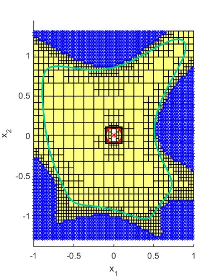
For step 2 in Algorithm 1 we choose . We sample the set by hyper–rectangles such that initially , where . We obtain the following: , is the yellow set illustrated in Fig. 4. The white set around the origin is .
Fix the neighborhood . We verify via fmincon, in Matlab, that the quadratic Lyapunov function found for the system linearized in 0 (via dlyap, in Matlab) is also a Lyapunov function for the nonlinear system in . The maximum level set of the Lyapunov function , of value 0.0133, which is inside , is an invariant set . is illustrated with black boundary, with red boundary. The Lyapunov function, as in (7), is and the set illustrated with green boundary, i.e., the largest levelset of (of value , where and ) which is still contained in , estimated according to Section IV-B, is subset of the DOA of the origin.
With blue we have illustrated the points which did not satisfy (11) in Theorem III.4 after multi–resolution sampling with . Simulations of the dynamics starting from these points shows indeed the convergence of most of these trajectories to other equilibria, and not to the origin. Convergence to the maximum can be achieved for . Notice in Fig. 4 also the multi–resolution sampling of the set . As expected, a more fine resolution is needed towards the boundary of , both towards the outer and the inner boundary.
Notice that the set obtained with the method in this paper is larger than the DOA estimate obtained in [27]. Also, while in [20] a total number of sample points were verified, in this paper, only sample points were explored, because of the freedom of choosing any rectangle as a sampling unit, which we can maximize in such a manner that we obtain no overlay of the yellow hyper–rectangles, in the construction of , as opposed to the unnecessary intersections in [20].
V-B Piecewise continuous nonlinear system

To illustrate the method proposed in this paper for verification of a piecewise continuous nonlinear system, consider again Example 1. Let the search space be
Provide as input in Algorithm 2 the values , . Choose a candidate function . By applying Algorithm 2 to Example 1, we obtain the results illustrated in Fig. 5. is the yellow set. With blue we have illustrated the points which did not satisfy (11). The Lyapunov function, found as in (7), is The white set around the origin is .
We linearize in 0 by linearizing both dynamics and in 0. We obtain a switched linear system, for which with is a common Lyapunov function. We choose and via fmincon, in Matlab, we verify that the quadratic Lyapunov function found for the system linearized in 0 is also a Lyapunov function for the nonlinear system in the neighborhood . The maximum level set of in is , which gives the local invariant set , illustrated with red.
The set illustrated with green boundary is the levelset of the Lyapunov function , computed according to Section IV-B and it is subset of the DOA of the origin. Here, , , and therefore . To compute , we sampled with a distance between samples of value 0.01. Therefore, for a point on the vertical boundary of , , while for a point on the horizontal boundary of , . provides an underestimation of the true largest levelset of , of value , depicted in Fig. 5 with magenta, which is still contained in . The relatively low quality of the estimation of the levelset, in this case, is due to the large .
In this example, in step 2 of Algorithm 1 we choose , which is on the switching boundary. The basic sampling unit is a hyper–cube. Note, however, that . Moreover, by multi–resolution, the samples chosen by the algorithm are not on the switching boundary. Therefore, for all . Furthermore, the switching boundaries can always be avoided by choosing a sample outside of the boundary.
In comparison to the results obtained in [22, Example 4], the DOA computed here is larger in set , but smaller in the set . Note that in this paper we aim at verifying Lyapunov inequalities and at computing a subset of DOA, without claiming to maximize it.
V-C 3D model
The following example illustrates the developed methodology on a 3D system, both in discrete–time, and in continuous–time. The system, see [28], is defined by:
which will be here discretized via the Euler method, i.e., , where is the discretization step.
Let the search space be
Consider and . Choose a candidate FSLF, with . The choice is motivated by the fact that the largest possible ellipsoid that can be contained in the given box is a level set of . Take .
We sampled here via hyper–cubes, and we obtain the following: , the points in the box which did not satisfy (11) in Theorem III.4 are illustrated with blue.
Fix the neighborhood . Again, we check via fmincon, in Matlab, that the quadratic Lyapunov function
found for the system linearized in 0 (via dlyap, in Matlab) is also a Lyapunov function for the nonlinear system in . The maximum level set of the Lyapunov function , of value 0.81, which is inside , is an invariant set , illustrated in Fig. 6 by the red ellipsoid.

The Lyapunov function found with this procedure is The set , illustrated with green, is the largest estimated levelset of (of value , where and ) which is still contained in . is subset of the DOA of the origin.
Moreover, by applying Algorithm 4, we obtain that is also subset of the DOA of the original continuous–time system. For the continuous–time system, , therefore, will differ, with a new value . has the same value as previously, i.e., , because the set remains the same, and thus , which means that .
It is noticeable that the set contains also regions of the state space which are not found in the DOA computed in [28] for the original continuous–time system, see, e.g., the black trajectory illustrated in Fig. 6, having as initial state one of the points which was not captured in [28], but which belongs to .
V-D Powertrain Control System
This example illustrates the potential of the methodology developed in this paper for computing the DOA of the origin for a system inspired by a real–life application. Consider a 3D simplified version of a Powertrain Control system, inspired by Example 5 of [11]:
where is the state vector. Here is the pressure manifold, is the air–to–fuel ratio and is a PI controller, designed to maintain the air–to–fuel ratio in of the optimal value. The corresponding parameters are: , , , , , , , , , , , . We aim to compute a set where the control system maintains the performance specification of keeping the air–to–fuel ratio in of the optimal value.

The continuous–time system will be again discretized via the Euler method, i.e., , where is the discretization step. The equilibrium is translated in 0, and we study the –stability of 0, and its corresponding DOA.
Let the search space be Choose the inputs and . Choose a candidate FSLF, with , and .
We obtain the following: , is the gray set illustrated in Fig. 7, excluding the balls , where are the blue points in the box which did not satisfy (11) in Theorem III.4. However, we certify with by optimization in each of the sets via fmincon.
fmincon fails to provide us with certification for a local Lyapunov function . Thus we have no invariant set . Thus, Theorem IV.4 is not used here, because set is the union of all the sets certified via fmincon and the set certified via Theorem III.4, which implies that holds for all .
The Lyapunov function we find is and the set illustrated with green, i.e., the largest levelset of (, computed with ) which is still contained in , is subset of the DOA of the origin for the discretized system.
By applying Algorithm 4, we obtain that is also subset of the DOA of the original continuous–time system, because , which means also that the new levelset of is the same as computed previously for the discretized system, i.e., . This fact guarantees that, for any initial condition starting in , , for all , which means that, indeed, for any initial condition starting in , air–to–fuel ratio is maintained in of the optimal value.
VI Conclusions
In this paper, a sampling–based approach to stability verification for hybrid nonlinear systems via Lyapunov functions was proposed, to avoid large, possibly non–feasible optimization problems involved in finding Lyapunov functions. This constructive approach, applicable to both discrete–time and continuous–time systems, proposes verification of the decrease condition for a candidate Lyapunov function on a finite sampling of a bounded set of initial conditions and then it extends the validity of the Lyapunov function to an infinite set of initial conditions by exploiting continuity properties. Multi–resolution sampling is employed to perform efficient state–space exploration and hyper–rectangles are used as basic sampling blocks, to account for different constraint scale on different states and further reduce the amount of samples to be verified. This verification method is decentralized in the sampling points, which makes the method scalable to any degree. The potential of the proposed methodology was illustrated through examples.
References
- [1] T. X. T. Dang, “Verification and synthesis of hybrid systems,” Ph.D. dissertation, Institut National Polytechnique de Grenoble-INPG, 2000.
- [2] A. Girard, “Reachability of uncertain linear systems using zonotopes,” in Hybrid Systems: Computation and Control. Springer, 2005, pp. 291–305.
- [3] M. Althoff, O. Stursberg, and M. Buss, “Verification of uncertain embedded systems by computing reachable sets based on zonotopes,” in Proc. of the 17th IFAC World Congress, 2008, pp. 5125–5130.
- [4] ——, “Reachability analysis of nonlinear systems with uncertain parameters using conservative linearization,” in Decision and Control, 2008. CDC 2008. 47th IEEE Conference on. IEEE, 2008, pp. 4042–4048.
- [5] C. Fan and S. Mitra, “Bounded verification with on-the-fly discrepancy computation,” in International Symposium on Automated Technology for Verification and Analysis. Springer, 2015, pp. 446–463.
- [6] J. Kapinski and J. Deshmukh, “Discovering forward invariant sets for nonlinear dynamical systems,” in Proceedings of the International Conference on Applied Mathematics, Modeling and Computational Science, 2013.
- [7] J. A. W. van cler Spek, “Cell mapping methods: modifications and extensions,” Ph.D. dissertation, 1994.
- [8] Á. Castillo and P. J. Zufiria, “Cell mapping techniques for tuning dynamical systems,” in Global Analysis of Nonlinear Dynamics. Springer, 2012, pp. 31–50.
- [9] H. K. Khalil, Nonlinear systems. Prentice hall Upper Saddle River, 2002, vol. 3.
- [10] M. Vidyasagar, Nonlinear systems analysis. Siam, 2002, vol. 42.
- [11] J. Kapinski, J. V. Deshmukh, S. Sankaranarayanan, and N. Arechiga, “Simulation-guided Lyapunov analysis for hybrid dynamical systems,” in Proceedings of the 17th international conference on Hybrid systems: computation and control. ACM, 2014, pp. 133–142.
- [12] U. Topcu, A. Packard, and P. Seiler, “Local stability analysis using simulations and sum-of-squares programming,” Automatica, vol. 44, no. 10, pp. 2669–2675, 2008.
- [13] S. Gao, J. Avigad, and E. M. Clarke, “-complete decision procedures for satisfiability over the reals,” in Automated Reasoning. Springer, 2012, pp. 286–300.
- [14] L. De Moura and N. Bjørner, “Z3: An efficient SMT solver,” in Tools and Algorithms for the Construction and Analysis of Systems. Springer, 2008, pp. 337–340.
- [15] B. Akbarpour and L. C. Paulson, “Metitarski: An automatic theorem prover for real-valued special functions,” Journal of Automated Reasoning, vol. 44, no. 3, pp. 175–205, 2010.
- [16] F. Berkenkamp, R. Moriconi, A. P. Schoellig, and A. Krause, “Safe learning of regions of attraction for uncertain, nonlinear systems with gaussian processes,” in 55th IEEE Conference on Decision and Control, Las Vegas, USA, 2016.
- [17] E. Najafi, R. Babuška, and G. A. Lopes, “A fast sampling method for estimating the domain of attraction,” Nonlinear Dynamics, pp. 1–12, 2016.
- [18] R. Geiselhart, R. H. Gielen, M. Lazar, and F. R. Wirth, “An alternative converse Lyapunov theorem for discrete-time systems,” Systems and Control Letters, vol. 70, no. 0, pp. 49 – 59, 2014.
- [19] R. V. Bobiti and M. Lazar, “A delta–sampling verification theorem for discrete–time, possibly discontinuous systems,” in 18th International Conference on Hybrid Systems: Computation and Control, Seattle, Washington, USA, 2015.
- [20] ——, “A sampling approach to finding Lyapunov functions for nonlinear discrete-time systems,” in European Control Conference, Aalborg, Denmark, 2016.
- [21] ——, “On the computation of Lyapunov functions for discrete–time nonlinear systems,” in 18th International Conference on System Theory, Control and Computing, Sinaia, Romania, 2014.
- [22] C.-k. Luk, “Domain of attraction in hybrid systems,” HKU Theses Online (HKUTO), 2015.
- [23] L. Jaulin, M. Kieffer, O. Didrit, and E. Walter, Applied Interval Analysis. Springer, 2001.
- [24] R. E. Moore, R. B. Kearfott, and M. J. Cloud, Introduction to interval analysis. Siam, 2009.
- [25] S. Rump, “INTLAB - INTerval LABoratory,” in Developments in Reliable Computing, T. Csendes, Ed. Dordrecht: Kluwer Academic Publishers, 1999, pp. 77–104. [Online]. Available: http://www.ti3.tuhh.de/rump/
- [26] F. Blanchini and S. Miani, Set-theoretic methods in control. Springer Science & Business Media, 2007.
- [27] P. Giesl, “On the determination of the basin of attraction of discrete dynamical systems,” Journal of Difference Equations and Applications, vol. 13, no. 6, pp. 523–546, 2007.
- [28] J. Björnsson, S. Gudmundsson, and S. Hafstein, “Class library in c++ to compute lyapunov functions for nonlinear systems,” IFAC-PapersOnLine, vol. 48, no. 11, pp. 778–783, 2015.
- [29] M. Berz and G. Hoffstätter, “Computation and application of Taylor polynomials with interval remainder bounds,” Reliable Computing, vol. 4, no. 1, pp. 83–97, 1998.
APPENDIX
In what follows we will need to use the Mean Value Theorem to process the Taylor series expansion in (18), see [29, Section 2]. However, the Mean Value Theorem can not be directly applied to multivariate functions, and therefore a one–dimensional function is introduced by the formula , where and are given. Note that
and
Denote
Notice that the formulae of and are similar, but is multivariate, while is univariate. Furthermore
Apply Taylor expansion formula to around and evaluate in :
Let us apply the Mean Value Theorem to and an arbitrary function with on . There exists such that:
and therefore
| (43) |
To analyse the expression of when we derivate with respect to the second argument we see that
| (44) |
If , then . Notice that for . Then, from (43) and (44) it follows that
where
| (45) |
is the Lagrange remainder and .