The Bayesian SLOPE

The posterior distribution of the vector of coefficients equals

which is proportional to the density of a multivariate normal distribution for any fixed order of $\{|\beta_{i}|;i=1,\ldots,p\}$ and signs of the coefficients $\{\beta_{i};i=1,\ldots,p\}$. To make the statement precise, for a permutation $\tau\in\mathcal{S}_{p}$ and a sign vector $s\in\{\pm 1\}^{p}$, define

where $\mathcal{S}_{p}$ is the group of all permutations of the set $\{1,\ldots,p\}$ The posterior can be written as

which is a weighted sum of multivariate normal densities each restricted to one of the sets $\mathcal{O}_{\tau,s}$ for $\tau\in\mathcal{S}_{p}$ and $s\in\{\pm 1\}^{p}$. Denote by $\mathcal{N}^{\tau,s}(x\mid\mu,\Sigma)$ the multivariate normal density with mean vector $\mu$ and covariance matrix $\Sigma$, truncated to $\mathcal{O}_{\tau,s}$. The posterior can be written as

with the common covariance structure $\Sigma=\sigma^{2}(X^{T}X)^{-1}$ and the orthant-dependent means and weights

where $\hat{\beta}_{OLS}=(X^{T}X)^{-1}X^{T}y$ is the ordinary regression coefficient vector, $D_{\tau,s}$ is the signed permutation matrix corresponding to the permutation $\tau$ and signs vector $s$, and $m_{\tau,s}=\int\mathcal{N}^{\tau,s}(\beta\mid\mu_{\tau,s},\Sigma)d\beta$.

The model can be extended with specifying priors on variance of the noise. A typical choice for the prior on $\sigma^{2}$ is the inverse gamma prior

The model (1.3), along with (2.3), define a full Bayesian regression model with hyper-parameters $a,\gamma,\text{and }\lambda$. The full posterior can be sampled using Markov chain Monte Carlo methods discussed in Section 3.

Remark. Instead of the prior (2.3) on $\sigma^{2}$, one can use the non-informative improper prior $\pi(\sigma^{2})\propto 1/\sigma^{2}$, which is a special case of (2.3) with $a=\gamma=0$. This choice of prior induces a proper posterior and the joint posterior for $(\beta,\sigma^{2})$ is again unimodal, which can be sampled similarly to the posterior resulting from (2.3).

The posterior distribution of $(\beta,\sigma^{2})$ is usually the main object of interest in a Bayesian regression problem. However, one might carry out a Bayesian analysis about the regularization coefficients too, to take into account other types of prior information available. Choosing a reasonable prior on $\lambda$ depends on information the practitioner has. A conjugate prior is proposed in Section 4.2. Empirical Bayes choice of $\lambda$ is discussed in Section 4.1.

Two major tasks of interest in linear regression problems are point estimation of the parameters and prediction of the response for future observations. The Bayesian point estimate of $\beta$, under a given loss function $\ell(\hat{\beta},\beta)$, is the estimator $\hat{\beta}$ minimizing the expected posterior loss, $\int\ell(\hat{\beta},\beta)\pi(\beta\mid\sigma^{2},\lambda,y)d\beta$. Common choices are the posterior mean and median, which are the point estimates corresponding to squared-error loss and absolute-error loss functions, respectively. The SLOPE estimate, $\hat{\beta}_{SLOPE}$, corresponds to the posterior mode. Although using the posterior mode as a Bayesian point estimate has become more popular recently, it seems to be an unnatural choice for a Bayesian statistician. Particularly, it can be realized as the $\epsilon\downarrow 0$ limit of Bayes estimates corresponding to loss functions $1-\mathbb{I}_{\|\hat{\beta}-\beta\|<\epsilon}$. Although choosing the loss function is subjective and up to the statistician, this choice of loss function seems rather unnatural.

Equally important is the task of predicting the response for new observations. Consider a new observation $X_{0}$ at which one wishes to predict the response. The Bayesian prediction of the future value is made using the posterior predictive distribution,

For a loss function $\ell(\tilde{y},y_{0})$, the Bayesian prediction is based on the predictor $\tilde{y}$ minimizing the expected posterior predictive loss,

Under the squared-error loss the prediction is done using the mean of the posterior predictive distribution, given by $\tilde{y}=X_{0}\mathbb{E}(\beta\mid\sigma^{2},\lambda,y)$. An important advantage of the squared-error loss is the fact that the posterior mean provides both point estimation and prediction. On the other hand, the mode of the posterior predictive distribution, $p(y_{0}\mid\sigma^{2},\lambda,y)$, is not equal to $X_{0}\hat{\beta}_{SLOPE}$. An example in which this is the case for the univariate lasso problem is provided in [17]. The popular prediction rule given by $\tilde{y}=X_{0}\hat{\beta}_{SLOPE}$, although useful, does not seem to have a solid Bayesian justification. The posterior mean is a more natural choice for prediction.

The Gibbs sampler is the most commonly used sampling method in Bayesian analysis. Most of the Bayesian variable selection methods mentioned in Section 1 use Gibbs sampling to sample from the posterior. A Gibbs sampler for the SLOPE posterior, which updates each parameter on at a time, is described in this Section. The direct characterization of the posterior, (2.2), is used to compute the conditional posterior for $\beta_{j}$, which is piecewise normal. For a fixed $j$, let $x_{1}\geq\ldots\geq x_{p-1}$ be the sorted values of $\{|\beta_{i}|\mid i\neq j\}$. For $k=1,\ldots,p$, let $\mathcal{N}^{k}(.\mid\mu,\eta^{2})$ and $\mathcal{N}^{-k}(.\mid\mu,\eta^{2})$ be the normal density with mean $\mu$ and variance $\eta^{2}$ truncated to $[x_{k},x_{k-1})$ and $(-x_{k-1},-x_{k}]$, respectively, where $x_{0}=\infty$ and $x_{p}=0$. With this notation, the conditional posterior distributions are

The weights and means in (3.1) are (for $s=\pm 1,\,\,k=1,\ldots,p$)

where $\omega_{ij}$ is the $ij$ entry of $\Sigma^{-1}$ . The parameters in (3.2) are

The conditional posterior for $\beta_{j}$ can be sampled using the piecewise normal characterization (3.1). Since the mean parameters in (3.3) change only slightly at each iteration, we only need to update the previous values, which requires linear number of operations in $p$. The weights in (3.4) can be updated in linear time too, thus, each run through the entire vector $\beta$ requires quadratic number of operations. Thus, the Gibbs sampler is affordable for moderately large $p$. Sampling from the conditional distribution of $\sigma^{2}$ is discussed in the appendix of [17].

The Gibbs sampler can be initialized at $(\beta_{in},\sigma^{2}_{in})=(\hat{\beta}_{SLOPE},\hat{\sigma}^{2})$, where $\hat{\beta}_{SLOPE}$ is the SLOPE estimate and $\hat{\sigma}^{2}$ is an estimate of the variance from the data. A systematic scan can be used, sampling in the following order: $\beta_{j}$ for $j=1,2,\ldots,p$ and then $\sigma^{2}$.

Although implementing the standard Gibbs sampler is straightforward, in some cases, e.g. when the predictor variables are highly correlated, it can suffer from high autocorrelation. Another limitation, in a large $p$ setting, is the relatively high cost of sampling the conditional distribution for $\beta_{j}$. Despite the complicated posterior $\pi(\beta\mid\sigma^{2},\lambda,y)$, the usual block-updating solution is feasible, thanks to recent developments in Markov chain Monte Carlo simulation. This is presented in Section 3.2.

The Gibbs sampler from Section 3.1 can be improved to a block-updating Gibbs sampler using the Hamiltonian Monte Carlo [14, 27], to sample directly from the multivariate conditional distribution $\pi(\beta\mid\sigma^{2},\lambda,y)$. To sample from a distribution $p(x)=e^{-U(x)}$ on $\mathbb{R}^{p}$, Hamiltonian Monte Carlo expands the parameter space by adding a ‘momentum’ variable $v\in\mathbb{R}^{p}$. It samples the momentum from the standard Gaussian distribution and evolves the current state $(x,v)$ by running the Hamiltonian dynamics

with initial condition $(x_{0},v_{0})$. After a fixed time $T$, the location component $x_{T}$ is kept and the momentum component $v_{T}$ is re-sampled. In most applications the Hamilton equations are not exactly solvable; hence a numerical approximation is needed. The most popular numerical method is the leapfrog procedure. To account for the approximation error, a Metropolis-Hasting correction is usually used, see [27] for more details. Hamiltonian Monte Carlo is implemented efficiently in the software system STAN [8].

It might be possible to improve upon the generic Hamiltonian Monte Carlo implementations by avoiding the rejections from the Metropolis-Hasting filter. Pakman and Paninski [28] provide exact solutions of the Hamilton equations for the case of the truncated (multivariate) normal distribution. This method can be directly used for the SLOPE posterior $\pi(\beta\mid\sigma^{2},\lambda,y)$. There is slight subtlety because of the non-smoothness of the posterior for $\beta$, i.e. lack of differentiablity at $\beta_{i}=0$ and $\beta_{i}=\beta_{j}$. Chaari et al. [13] have addressed this issue by introducing a Hamiltonian Monte Carlo for non-smooth log-densities, which uses sub-gradients instead of gradients. See [28, 13] for details.

Algorithm 1 describes a block-updating Gibbs sampler based on Hamiltonian Monte Carlo, which can be implemented in the STAN modeling language. A sampler based on Hamiltonian Monte Carlo is implemented in STAN and is available as online supplement, which also provides the R functions required to run Algorithm 1.

The model defined by (1.3) and (2.3) induces a likelihood function for $\lambda$. This likelihood function, computed on the observed data $(X,y)$, can be used to obtain a frequentist estimate of $\lambda$ via Expectation-Maximization (EM) algorithm. In general, for almost all problems, there is no guarantee that the EM algorithm converges to the maximum likelihood estimator, but it increases the likelihood at each step. The full-data log-likelihood is

The E-step in the EM algorithm computes the expected value of this log-likelihood given $y$, under the distribution with current iterate $\lambda^{k}$, to get

The M-step maximizes $Q(\lambda\mid\lambda^{k})$ over $\lambda$ to update the iterate to $\lambda^{k+1}=\text{arg}\max_{\lambda}Q(\lambda\mid\lambda^{k})$. This is a convex optimization problem in $\lambda$ and can be solved efficiently using gradient decent and alternating direction method of multipliers . The EM algorithm is repeated until a desired level of convergence is obtained, i.e. $\|\lambda^{k-1}-\lambda^{k}\|<\epsilon$. For the Bayesian SLOPE, the EM algorithm is hard to carry out, as there is no analytical expression for $\mathbb{E}_{\lambda^{k-1}}\left[|\beta|_{(i)}/\sigma\mid y\right]$. The expectations in the E-step can be computed using Monte Carlo methods; this procedure is called the Monte Carlo EM algorithm [10]. For the Bayesian SLOPE, the steps are described in algorithm 2.

This Section considers a Bayesian treatment of the penalty parameter, $\lambda$. It is indeed essential to incorporate any educated suggestion and prior knowledge into the prior distribution of $\lambda$. In the case there is not much known a priori, a generic proposal can be used. For a set of parameters $b_{1},\ldots,b_{p}$ and $c_{1},\ldots,c_{p}$, define

which induces a proper prior if $b_{i}>0$, $c_{i}\geq 0$, for $i=1,\ldots,p$. Under the model (1.3), the posterior is

The Gibbs sampler can be modified to handle sampling from (4.2). The conditional posterior distribution of $\lambda_{j}$ is

The conditional posterior (4.3) can be sampled through rejection sampling using the truncated exponential distribution as the reference distribution. Details are given in Appendix B.1.

The hybrid sampler also can be extended to facilitate sampling from (4.2). Instead of sampling $\lambda$ one coordinate at a time, sample it all at once using Hamiltonian Monte Carlo. The resulting algorithm is described below.

In algorithm 3, $\lambda_{BH}$ is the vector of regularization coefficients used by the SLOPE. The Bayesian model with a hyperprior on $\lambda$ is also implemented in STAN modeling language. It can be used along with the STAN package to run algorithm 3 for a generic regression problem, which makes reproducible research more feasible.

This section compares the SLOPE and the Bayesian SLOPE estimates for simulated data sets. The first experiment involves $200$ observations of $80$ predictors and a response. The design matrix $X$ has independent standard normal entries, the regression coefficients $\beta$ are

and the errors are standard normal. Both estimates are obtained using the vector of tuning parameters

The posterior mean is used as the Bayesian point estimate along with the symmetric credible sets. The point estimates along with the $95\%$ Bayesian credible sets are illustrated in Figure 1. As can be seen in Figure 1, the credible sets cover the true value for most of the variables. There are $5$ non-coverages out of $80$ coefficients, which is expected at the $95\%$ credibility level. The Bayesian SLOPE and the SLOPE estimates agree on all of the coefficients to a great extent.

The closely matching estimates suggests that the two estimates should behave similarly in predicting the response for future observations. In fact, the Bayesian and empirical Bayes SLOPE estimates, and the SLOPE estimate exhibit similar predictive performance in this example. The out of sample prediction is studied by fitting the three models on a randomly chosen train/test split of the data into groups of 160 and 40 observations; repeated 10 times, using the sum of squares predictive loss function. The estimated prediction errors are presented below in Table 1. In this simulated data set, the two methods perform similarly in terms of estimation and prediction.

This Section considers the Diabetes data set used by Efron et al. [15]. The data set includes 442 observations on 10 predictor variables and a response variable. The standardized version of the design matrix has been used. The Bayesian SLOPE has been fitted and compared with the SLOPE and least squares; the result is summarized in Table 2. Individual kernel posterior density estimates are illustrated in Figure 2.

The Bayesian SLOPE seems to shrink more than the SLOPE. Interesting, there are some noticeable discrepancies between them for some of the coefficients. However, this does not cause conceptual problems because the variables for which there is a significant disagreement are highly correlated. Particularly, we have $corr(X_{5},X_{6})\approx 0.90$, $corr(X_{7},X_{8})\approx 0.74$, and $corr(X_{6},X_{8})\approx 0.66$. It is generally problematic to have highly correlated predictors in the model. Each method estimates differently on the correlated variables. For example, the least squares and the SLOPE provide relatively large values for $X_{5}$ and $X_{6}$, with different signs, which cancel out because of the correlation. On the other hand, the Bayesian SLOPE estimates both coefficients with relatively small negative values. A similar effect is present for $X_{7}$ and $X_{8}$. The two methods would provide more similar estimates if the correlated pairs were replaced by a linear mixture each. One would expect that highly correlated predictors should result in a posterior with high correlation between corresponding coefficients. This is indeed the case for the Diabetes data set; and can be seen in Figure 3, which illustrates the pairwise posterior correlations between the regression coefficients.

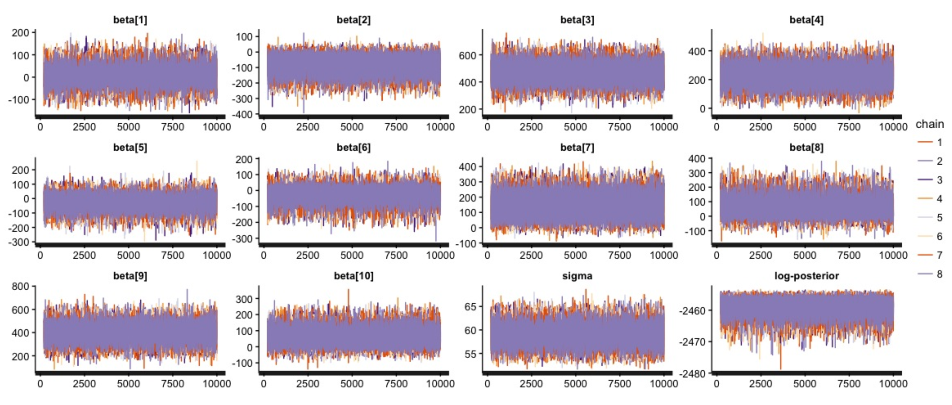
The Hamiltonian Monte Carlo sampler, implemented using STAN, exhibits desirable convergence even after 1000 steps. The results in this Section are obtained based on 10000 steps of 8 parallel chains. For 10000 steps, the lag-three auto-correlation for all the chains is less than $0.02$. A variety of convergence diagnostics are provided in the output from STAN. For instance, Figure 4 shows the trace plots of the MCMC sampler for the parameters $\beta$ and $\sigma$.

References

- [1] Pierre C Bellec, Guillaume Lecué, and Alexandre B Tsybakov. Slope meets lasso: improved oracle bounds and optimality. arXiv preprint arXiv:1605.08651, 2016.
- [2] Yoav Benjamini and Yosef Hochberg. Controlling the false discovery rate: a practical and powerful approach to multiple testing. Journal of the Royal Statistical Society. Series B (Methodological), pages 289–300, 1995.
- [3] Anirban Bhattacharya, Debdeep Pati, Natesh S Pillai, and David B Dunson. Dirichlet–laplace priors for optimal shrinkage. Journal of the American Statistical Association, 110(512):1479–1490, 2015.
- [4] Anirban Bhattacharya, David B Dunson, Debdeep Pati, and Natesh S Pillai. Sub-optimality of some continuous shrinkage priors. arXiv preprint arXiv:1605.05671, 2016.
- [5] Małgorzata Bogdan, Ewout van den Berg, Chiara Sabatti, Weijie Su, and Emmanuel J Candès. Slope—adaptive variable selection via convex optimization. The annals of applied statistics, 9(3):1103, 2015.
- [6] Luke Bornn, Raphael Gottardo, and Arnaud Doucet. Grouping priors and the bayesian elastic net. arXiv preprint arXiv:1001.4083, 2010.
- [7] Peter Carbonetto and Matthew Stephens. Scalable variational inference for bayesian variable selection in regression, and its accuracy in genetic association studies. Bayesian analysis, 7(1):73–108, 2012.
- [8] Bob Carpenter, Andrew Gelman, Matt Hoffman, Daniel Lee, Ben Goodrich, Michael Betancourt, Michael A Brubaker, Jiqiang Guo, Peter Li, and Allen Riddell. Stan: A probabilistic programming language. J Stat Softw, 2016.
- [9] Carlos M Carvalho, Nicholas G Polson, and James G Scott. The horseshoe estimator for sparse signals. Biometrika, page asq017, 2010.
- [10] George Casella. Empirical bayes gibbs sampling. Biostatistics, 2(4):485–500, 2001.
- [11] Ismaël Castillo and Aad van der Vaart. Needles and straw in a haystack: Posterior concentration for possibly sparse sequences. The Annals of Statistics, 40(4):2069–2101, 2012.
- [12] Ismaël Castillo, Johannes Schmidt-Hieber, and Aad Van der Vaart. Bayesian linear regression with sparse priors. The Annals of Statistics, 43(5):1986–2018, 2015.
- [13] Lotfi Chaari, Jean-Yves Tourneret, Caroline Chaux, and Hadj Batatia. A hamiltonian monte carlo method for non-smooth energy sampling. arXiv preprint arXiv:1401.3988, 2014.
- [14] Simon Duane, Anthony D Kennedy, Brian J Pendleton, and Duncan Roweth. Hybrid monte carlo. Physics letters B, 195(2):216–222, 1987.
- [15] Bradley Efron, Trevor Hastie, Iain Johnstone, Robert Tibshirani, et al. Least angle regression. The Annals of statistics, 32(2):407–499, 2004.
- [16] Mario AT Figueiredo and Robert D Nowak. Sparse estimation with strongly correlated variables using ordered weighted l1 regularization. arXiv preprint arXiv:1409.4005, 2014.
- [17] Chris Hans. Bayesian lasso regression. Biometrika, 96(4):835–845, 2009.
- [18] Chris Hans. Model uncertainty and variable selection in bayesian lasso regression. Statistics and Computing, 20(2):221–229, 2010.
- [19] Chris Hans. Elastic net regression modeling with the orthant normal prior. Journal of the American Statistical Association, 106(496):1383–1393, 2011.
- [20] Daniel Hernández-Lobato, José Miguel Hernández-Lobato, and Pierre Dupont. Generalized spike-and-slab priors for bayesian group feature selection using expectation propagation. Journal of Machine Learning Research, 14(1):1891–1945, 2013.
- [21] Hemant Ishwaran and J Sunil Rao. Spike and slab variable selection: frequentist and bayesian strategies. Annals of Statistics, pages 730–773, 2005.
- [22] Hemant Ishwaran and J Sunil Rao. Consistency of spike and slab regression. Statistics & Probability Letters, 81(12):1920–1928, 2011.
- [23] Qing Li and Nan Lin. The bayesian elastic net. Bayesian Analysis, 5(1):151–170, 2010.
- [24] Qing Li, Ruibin Xi, and Nan Lin. Bayesian regularized quantile regression. Bayesian Analysis, 5(3):533–556, 2010.
- [25] Ryan Martin and Stephen G Walker. Asymptotically minimax empirical bayes estimation of a sparse normal mean vector. Electronic Journal of Statistics, 8(2):2188–2206, 2014.
- [26] Elías Moreno, Javier Girón, and George Casella. Posterior model consistency in variable selection as the model dimension grows. Statistical Science, 30(2):228–241, 2015.
- [27] Radford M Neal. Mcmc using hamiltonian dynamics. Handbook of Markov Chain Monte Carlo, 2:113–162, 2011.
- [28] Ari Pakman and Liam Paninski. Exact hamiltonian monte carlo for truncated multivariate gaussians. Journal of Computational and Graphical Statistics, 23(2):518–542, 2014.
- [29] Trevor Park and George Casella. The bayesian lasso. Journal of the American Statistical Association, 103(482):681–686, 2008.
- [30] Nicholas G Polson and James G Scott. Shrink globally, act locally: sparse bayesian regularization and prediction. Bayesian Statistics, 9:501–538, 2010.
- [31] Nicholas G Polson, James G Scott, and Jesse Windle. The bayesian bridge. Journal of the Royal Statistical Society: Series B (Statistical Methodology), 76(4):713–733, 2014.
- [32] Vikas C Raykar and Linda H Zhao. Nonparametric prior for adaptive sparsity. In AISTATS, pages 629–636, 2010.
- [33] Veronika Rocková. Bayesian estimation of sparse signals with a continuous spike-and-slab prior. Submitted manuscript, pages 1–34, 2015.
- [34] Veronika Rocková and E George. The spike-and-slab lasso. Manuscript in preparation, 2014a.
- [35] Veronika Rocková and Edward I George. Emvs: The em approach to bayesian variable selection. Journal of the American Statistical Association, 109(506):828–846, 2014b.
- [36] Veronika Rocková and Edward I George. Bayesian penalty mixing: The case of a non-separable penalty. In Statistical Analysis for High-Dimensional Data, pages 233–254. Springer, 2016.
- [37] James G Scott and James O Berger. Bayes and empirical-bayes multiplicity adjustment in the variable-selection problem. The Annals of Statistics, 38(5):2587–2619, 2010.
- [38] Weijie Su and Emmanuel Candes. Slope is adaptive to unknown sparsity and asymptotically minimax. arXiv preprint arXiv:1503.08393, 2015.
- [39] Robert Tibshirani. Regression shrinkage and selection via the lasso. Journal of the Royal Statistical Society. Series B (Methodological), pages 267–288, 1996.
- [40] SL van der Pas, BJK Kleijn, and AW van der Vaart. The horseshoe estimator: Posterior concentration around nearly black vectors. Electronic Journal of Statistics, 8(2):2585–2618, 2014.
- [41] Xiaofan Xu and Malay Ghosh. Bayesian variable selection and estimation for group lasso. Bayesian Analysis, 10(4):909–936, 2015.
- [42] Tso-Jung Yen. A majorization-minimization approach to variable selection using spike and slab priors. The Annals of Statistics, pages 1748–1775, 2011.