SPIDERS: the spectroscopic follow-up of X-ray selected clusters of galaxies in SDSS-IV
Abstract
SPIDERS (The SPectroscopic IDentification of eROSITA Sources) is a program dedicated to the homogeneous and complete spectroscopic follow-up of X-ray AGN and galaxy clusters over a large area (7500 deg2) of the extragalactic sky. SPIDERS is part of the SDSS-IV project, together with the Extended Baryon Oscillation Spectroscopic Survey (eBOSS) and the Time-Domain Spectroscopic Survey (TDSS). This paper describes the largest project within SPIDERS before the launch of eROSITA: an optical spectroscopic survey of X-ray selected, massive ( to ) galaxy clusters discovered in ROSAT and XMM-Newton imaging. The immediate aim is to determine precise () redshifts for 4,000–5,000 of these systems out to . The scientific goal of the program is precision cosmology, using clusters as probes of large-scale structure in the expanding Universe. We present the cluster samples, target selection algorithms and observation strategies. We demonstrate the efficiency of selecting targets using a combination of SDSS imaging data, a robust red-sequence finder and a dedicated prioritization scheme. We describe a set of algorithms and work-flow developed to collate spectra and assign cluster membership, and to deliver catalogues of spectroscopically confirmed clusters. We discuss the relevance of line-of-sight velocity dispersion estimators for the richer systems. We illustrate our techniques by constructing a catalogue of 230 spectroscopically validated clusters (), found in pilot observations. We discuss two potential science applications of the SPIDERS sample: the study of the X-ray luminosity-velocity dispersion () relation and the building of stacked phase-space diagrams.
Keywords:
cosmology: observations – catalogues – galaxies: clusters: general – X-rays: galaxies: clusters.1 Introduction
In recent years the field of galaxy cluster surveys has been re-energised by the realisation that a well-measured cluster population places strong independent constraints on cosmological models (Böhringer et al., 2004; Vikhlinin et al., 2009; Mantz et al., 2010; Weinberg et al., 2013, e.g.). As the largest known bound objects, clusters can be used to simultaneously probe the cosmic expansion rate and the gravitational mechanisms responsible for the growth of structure in the Universe. The evolution of the galaxy cluster mass function across cosmological times and the distribution of clusters within the tridimensional large-scale structure are two key observables, since they are readily predicted by theoretical models and simulations.
Galaxy cluster cosmology studies start with constructing cluster samples. Fortunately for observers, the hot baryonic gas trapped in galaxy clusters emits large amounts of X-ray photons, in great part due to bremsstrahlung processes. Extended X-ray objects are thus the signpost of deep potential wells, and their X-ray luminosity directly relates to the mass of the dark matter halo in which they reside. Therefore, large surveys of the sky at the high-energy end of the electromagnetic spectrum (i.e. X-ray) permit a complete census of clusters covering a wide range of masses and redshifts, and survey data themselves can provide estimates of the mass of these objects. This is why large surveys in the X-ray wavelengths aimed at constraining cosmology with galaxy clusters have been developed since the early years of X-ray astronomy (Henry & Arnaud, 1991; Bahcall & Cen, 1993; Jones & Forman, 1984), with a notable step-change brought about by the ROSAT all-sky survey (Ebeling et al., 2000; Ikebe et al., 2002; Reiprich & Böhringer, 2002; Schuecker et al., 2003) and ROSAT serendipitous surveys (Rosati et al., 1998; Romer et al., 2000; Burke et al., 2003; Burenin et al., 2007) and the support of Chandra and XMM-Newton (Pacaud et al., 2006; Vikhlinin et al., 2009; Mantz et al., 2010; Finoguenov et al., 2010; Clerc et al., 2014; Pierre et al., 2016). The next major advance in the field will be offered by eROSITA (Predehl et al., 2014, extended ROentgen Survey with an Imaging Telescope Array,) which will survey the entire sky in the 0.3-10 keV energy range at depths 10 to 30 times deeper than ROSAT. The combination of eROSITA’s field of view, angular resolution and sensitivity will lead to the detection of galaxy clusters down to keV fluxes of ergs s-1 cm-2 and up to redshifts of unity and beyond (Merloni et al., 2012; Borm et al., 2014, see).
However, X-ray observations alone, in general, are not sufficient to fully assess the nature of the emitting sources and, most importantly, to determine their redshifts. Therefore, optical observations play a critical role in complementing surveys of galaxy clusters in X-rays. Whilst multi-filter optical imaging proves efficient at detecting and characterizing galaxy clusters – notably through their ubiquitous red sequence (Gladders & Yee, 2000; Rykoff et al., 2014, e.g.) –, ultimate confirmation of a galaxy cluster is achieved by optical spectroscopy. Spectroscopic observations of cluster members can be used to disentangle projection effects and substructures from real concentrations, and they also provide the precise redshift of the halo, and therefore lead to precise luminosities and masses once they are combined with X-ray measurements. Obtaining spectroscopic redshifts for galaxy cluster members is recognized as a major bottleneck in X-ray cluster surveys, because of the double need for deep imaging data to select targets, and the deep spectroscopic exposures necessary for redshift determination.
The SPIDERS (SPectroscopic IDentification of eROSITA Sources) cluster program is specifically designed to overcome this bottleneck. It relies on the BOSS spectrograph mounted on the SDSS-2.5m telescope at Apache Point Observatory (Gunn et al., 2006) to follow-up galaxies detected in the large area of extragalactic sky imaged in filters by the same telescope. The SDSS/BOSS instrumentation and infrastructure are used in combination with most recent techniques in finding X-ray galaxy clusters and their photometric members, in order to perform an unprecedentedly wide spectroscopic survey of X-ray galaxy clusters. Advanced techniques used in this work include the wavelet filtering of X-ray maps, and the use of a series of matched filters to look for red-sequence galaxies in a multi-variate optical parameter space (colour, position and magnitude).
This paper (one of a series of SDSS-IV technical papers), describes the targeting and analysis steps leading to the construction of a large, spectroscopically validated sample of X-ray selected galaxy clusters within SPIDERS. In the preparation phase for eROSITA, these samples are drawn from ROSAT and XMM data. Throughout this paper we use a small pilot survey dubbed SEQUELS (Sloan Extended Quasar, ELG, and LRG Survey, a precursor to the main SPIDERS/eBOSS/TDSS program) to illustrate the efficacy of our targeting and analysis approach. We present the first scientific results from the SPIDERS cluster program.
The paper is structured as follows. Section 2 is devoted to the general presentation of the SPIDERS cluster survey and the samples of X-ray clusters it is based upon. The selection of targets for the shallower, pre-eROSITA phase of the survey is described in Sect. 3, along with forecasts regarding the outcome of the observations. In Sect. 4 we depict the steps envisaged to transform observations into science-oriented catalogues. We emphasize that these methods are subject to improvements in the course of the survey. In Section 5 we present some examples for the science exploitation of the SPIDERS program, using the validated sample of clusters from the SEQUELS pilot survey, that we compare to existing cluster catalogues in Sect. 6. We conclude in Sect. 7.
Unless otherwise stated, we assume a flat CDM cosmological model with , and km s-1 Mpc-1 with . We define , with and the [0.1-2.4] keV luminosity of a cluster.
2 The SPIDERS cluster program
2.1 General description
SPIDERS is an observational program, part of the SDSS-IV project (Blanton et al., 2017). The primary goal of SPIDERS is to obtain homogeneous and complete spectroscopic follow-up of extragalactic sources, both point-like and extended, using data from X-ray satellites and over the SDSS imaging footprint. Given the nature of these sources, SPIDERS naturally splits into two main components, i.e. an AGN program and a cluster program. The SPIDERS AGN targeting strategy is described in Dwelly et al. (in prep.), and will collect 50,000 spectra of ROSAT, XMM and eROSITA X-ray AGN. A pilot study for the SPIDERS AGN survey, based around the BOSS follow-up of X-ray selected AGN in the XMM-Newton XMM-XXL field, is presented in Menzel et al. (2016).
This paper describes the targeting of X-ray extended sources identified as galaxy cluster candidates. The driving goals of the program are the confirmation of those candidates and the assignment of a precise redshift. This in turn leads to the determination of precise absolute cluster parameters (including X-ray luminosity and mass). A number of important secondary goals include the estimation of cluster dynamical masses (via line-of-sight velocity dispersion measurements), the study of the physical interplay between massive dark matter halos, the hot baryonic gas they host, and the galaxies that live therein. From a technical point of view, the SPIDERS cluster program represents a novel approach to galaxy cluster spectroscopic follow-up: the large data volume involved (several thousands of galaxy clusters) demands innovative targeting and analysis strategies. Considering that the ultimate goal envisaged by the program is precision cosmology using galaxy clusters as tracers of the large-scale structure, we require that all the procedures involved must undergo careful control and validation.
SPIDERS will follow-up X-ray extended sources detected in eROSITA data in the final years of SDSS-IV. Prior to eROSITA’s launch, galaxy clusters identified in the shallower RASS and sparser XMM-Newton data will constitute the bulk of the SPIDERS program. There will be an incremental increase in X-ray sensitivity brought about by each of eROSITA’s sky surveys, which will start to be be accumulated after the start of SDSS-IV. Therefore, SPIDERS is planned in three tiers. Tier 0, the shallowest tier, relies mainly on ROSAT data. When successive eROSITA catalogues become available (following the cadence of one deeper X-ray catalogue every six months, going from eRASS:1 to eRASS:8), sources in the North Galactic Cap within the German eROSITA sky () will be added to the pool of targets. The planned launch date of eROSITA means that Tier 1 and Tier 2 will most likely correspond to eRASS depths 2 and 4 respectively. Fig. 1 shows the layout of the surveys in Equatorial coordinates. The area covered in Tier 0 corresponds to the entire eBOSS footprint not covered in Tiers 1 and 2, i.e. , while Tier 1 and 2 will lie to the South of the eROSITA-DE boundary (the black dashed curve in this figure), with exact footprints dependent on the launch date.
We detail in the following sub-sections the samples of galaxy clusters followed-up by SPIDERS in Tier 0, along with expectations regarding the deeper tiers, when eROSITA is available.


2.2 SPIDERS Tier 0: CODEX and XCLASS
Prior to the delivery of first cluster catalogues from eROSITA, SPIDERS ensures follow-up of galaxy clusters discovered in the RASS (ROSAT All-Sky Survey) and in XMM archival data. The two relevant cluster samples are the CODEX (Finoguenov et al., in prep.) and the XCLASS-RedMapper catalogue (Clerc et al., 2012; Sadibekova et al., 2014) respectively. Both are based on X-ray detections of galaxy clusters, yet they differ in their characteristics and their construction. Since they conveniently encompass the range of X-ray properties expected from eROSITA clusters (see below), they show a particular interest in view of preparing the eROSITA survey.
We provide details on their construction in the following paragraphs, and Table 1 summarizes the main characteristics of both samples. Note in particular that the same red-sequence finder was run for both samples.


2.2.1 The CODEX subsample
CODEX (COnstrain Dark Energy with X-ray clusters, Finoguenov et al., in prep.) is an extensive search for galaxy clusters in ROSAT data, based on the association of RASS photon overdensities to red-sequence galaxies identified in SDSS. It covers the entire SPIDERS/eBOSS footprint and these detections are expected to show as the brightest, best-characterized, cluster sources in future eROSITA data. The current study provides the only spectroscopically complete CODEX catalogue down to low richness values. As such, this paper is the first in a series of CODEX catalogue papers. The sample construction is fully detailed in Finoguenov et al. (in prep.) ; we briefly summarize here the steps leading to the list of cluster candidates.
As a first step, RASS data is searched for faint sources using a wavelet-based detection algorithm. The detection threshold is set to 4-. Sensitivity maps (as in Fig. 5) are created as by-products and help in assessing the completeness of the sample. On average, the 90% completeness level is achieved for a source delivering 8 X-ray counts, while the 10% completeness level is reached for sources delivering 4 counts. Given these sensitivity estimates, the number of spurious sources is estimated between 500 and 1000 across the entire CODEX area and the number of X-ray AGN amounts to around 20 000. The RedMapper algorithm (Rykoff et al., 2014) looks in SDSS imaging data (Data Release 8) for galaxies with similar colours around each faint RASS source, i.e. for a red-sequence formed by passive galaxies at the same redshift. This provides in turn an estimate for the photometric redshift of the cluster (based on the colours of the galaxies) and an optimized richness estimator. The counterpart having the highest richness is listed for each RASS X-ray source. Given the uncertain position of RASS detections the red-sequence algorithm is then run to optimally find the cluster center. The constraint on the centre position is relaxed, to be within from the X-ray position11 1 The mean and 95th percentile of the RASS faint point-source 1- positional uncertainty are and arcsec respectively.. The newly found red-sequence is used to provide a fresh estimate for the cluster photometric redshift and richness (optical or ”OPT” quantities: , etc.) In the final step, X-ray properties based on the RASS count-rate and the RedMapper redshift are calculated in optimized apertures (imposing a minimal signal-to-noise threshold of 1.6), assuming a model for the X-ray spectral emissivity. Among them stand the aperture-corrected cluster flux and keV luminosities .
The average number density of CODEX sources over the BOSS imaging footprint is 0.8 deg-2 (for candidates with richness22 2 By ’richness’ we will refer to the RedMapper richness estimator (Rykoff et al., 2014). It correlates with the total cluster mass and equals the sum of the membership probabilities of galaxies within a given system. ). Adding those with lower richness brings this number up to 1.0 deg-2. However, due to spatial fluctuations in the RASS depth, these numbers vary as a function of sky position.

2.2.2 The XCLASS-RedMapper subsample
XCLASS (Clerc et al., 2012, XMM CLuster Archive Super Survey,) is a search for galaxy clusters detected in the XMM-Newton archive, based on a robust cluster detection algorithm, developed in the context of the XMM-LSS (Pacaud et al., 2006; Clerc et al., 2014, e.g.) and XMM-XXL (Pierre et al., 2016) surveys. Extensive simulations of XMM observations, including realistic instrumental effects and astrophysical source populations, support the construction of a pure sample of extended objects in keV XMM images (the ”C1” selection, Pacaud et al. 2006). Visual screening removes nearby galaxies and detector artefacts, leading to the final catalogue of XCLASS galaxy cluster candidates. The L4SDB33 3 http://xmm-lss.in2p3.fr:8080/l4sdb/ database stores validated detections, along with other useful information related to the X-ray sources (redshifts, flux measurements, etc.) The XCLASS surveyed area amounts to deg2 but due to its very nature, it is scattered across the extragalactic sky (). All analyzed XMM observations were deliberately shrunk to 10 ks depths (exactly) so as to provide a survey as uniform as possible in sensitivity.
Sadibekova et al. (2014) performed the correlation of XCLASS C1 sources with the RedMapper optical cluster catalogue in the regions where the two surveys overlap. A major difference with the CODEX sample consists in very reliable cluster X-ray positions (the positional uncertainty amounts to a few arcsec rms), and the secure extended nature of the X-ray detections. Similarly to CODEX, the RedMapper algorithm provides an estimate for the photometric redshift and the optical richness () of the clusters. The SPIDERS sample contains 238 XCLASS clusters securely matched to a RedMapper candidate: i.e. and a correlation radius , or and . We further added a group of 40 less securely matched sources, having and .
The total number of XCLASS-RedMapper sources across the full SDSS imaging footprint amounts to 278, 84 of them are in common with the CODEX subsample described earlier. Since they are irregularly distributed on sky, their sky density is quoted over the common overlap area between XMM observations and the imaging footprint and amounts to 3-4 deg-2.
| CODEX | XCLASS-RedMapper | |
| Number of clusters in SDSS DR8 footprint | 10 415 | 278 |
| Sky distribution | Full SDSS area | Spatially scattered |
| Average candidate density () | 0.8 | 3-4(a) |
| Maximal redshift | ||
| Minimal richness | 10 (3(b)) | 5 |
| X-ray data origin | RASS faint sources | XMM-Newton archival data |
| X-ray selection | 4- above background | C1 selection (extended sources) |
| Limiting flux in X-rays (0.5–2 keV, units ergs/s/cm2) | ||
| X-ray positional accuracy | ||
| X-ray spatial resolution | ||
| X-ray energy resolution ( @ 1 keV) | eV | eV |
| Red-sequence finder | redMaPPer v.5.2 | redMaPPer v.5.2 |
| Optical search | Around each X-ray source | Independent from X-ray sources |
| Optical/X-ray association | Richness cut vs. chance identification | Angular distance criterion + visual checks |
 |
 |
2.3 eROSITA survey: eRASS samples
Although this paper focuses mainly on the targeting of Tier 0 samples, namely CODEX and XCLASS, we forecast our target budget for the future Tiers 1 & 2 in SPIDERS. These forecasts are based on pre-launch assumptions as for the amount and nature of eROSITA clusters (Merloni et al., 2012). A simple model, subject to the current uncertainty concerning the in-flight performances of the instrument and the actual physics of the population it will uncover, helps in deriving rough numbers and adjusting the targeting strategy. We modeled the galaxy cluster mass distribution using Tinker et al. (2008) halo mass function and converted masses () to X-ray temperatures and luminosities using scaling relations. The eROSITA selection is modeled with a lower cut in soft-band flux, representative of the selection relevant to each tier ( and ergs s-1 cm-2 for Tier 1 and 2 respectively). Integrating the resulting filtered mass distribution provided the curves shown in Fig. 2. The galaxy population within clusters was simulated by means of galaxy luminosity functions parametrized as a function of cluster mass and redshift (Popesso et al., 2005; Hansen et al., 2009). We folded a spectral energy distribution template representative of passive galaxies (Maraston et al., 2009) into the SDSS filter set. Flux losses due to the finite fiber aperture were accounted for by assuming a size-magnitude relation (Bernardi et al., 2007) and a typical seeing (see details in Zhang et al. 2016). We then applied a photometric selection representative of the SPIDERS target selection (see Sect. 3) and excluded galaxies whose photometric properties correspond to BOSS galaxy targets (Bolton et al., 2012, the LOWZ and CMASS selections ;). Finally, a cluster radius-dependent sampling factor was set to account for fiber collisions. The resulting redshift distribution of targetable galaxies not already targeted in BOSS is shown in Fig. 7, along with the densities of targets for each layer of the eROSITA survey. These numbers are indicative and are refined within the Tier 0 phase of SPIDERS.
Based on those calculations, SPIDERS (in its Tier 1 and 2 phases) will confirm 90% of eROSITA clusters by obtaining (at least) 3 spectroscopic redshifts per system (including those known from previous SDSS observations.) SPIDERS will also raise the number of spectroscopic members per cluster virial radius to 10 for 50% of the clusters and to 20 for 20% of the clusters.

2.4 The SEQUELS pilot program
SEQUELS (The Sloan Extended Quasar, ELG, and LRG Survey, Alam et al., 2015, their App. A.3) is an ancillary program part of BOSS (SDSS Data Release 12) and served as a pilot survey for the eBOSS, SPIDERS and TDSS programs in SDSS-IV (Dawson et al., 2016). Its initial footprint consists in the rectangle and . Only 300 deg2 of this area were observed (corresponding to 66 plates) as part of Data Release 12 (DR12, Alam et al., 2015, and Fig. 1). As a preparation for the SDSS-IV SPIDERS cluster follow-up program, SEQUELS contains a number of targets assigned to SPIDERS clusters. While the parent cluster samples are the same as for SPIDERS Tier 0 (i.e. CODEX and XCLASS), the target selection slightly differs and it is in general broader in SEQUELS (see Sect. 3). Throughout this work, we illustrate our envisaged analysis procedures with results extracted from the pilot SPIDERS program in SEQUELS DR12. Note that 51 SEQUELS plates (about ) are observed in the course of the eBOSS survey (post-DR12) and therefore the targeting strategy for those slightly differs from the main SPIDERS survey. These objects are not considered in the following ’pilot sample’.
3 Targeting strategy
This section details the steps followed in preparing the target lists in the first phase of SPIDERS (Tier 0). The main difference with respect to conventional multi-object spectroscopic observations of galaxy clusters, consists in an ensemble treatment of the entire pool of targets. Because the exact set of targets is only known after the eBOSS tiling algorithm has run (Dawson et al., 2016) and accommodated for the various target classes within eBOSS, we worked out a scheme for assigning priorities to potential targets, aimed at optimizing the primary science goal, namely the number of spectroscopically confirmed clusters.
3.1 Target selection and prioritization
3.1.1 The CODEX and XCLASS red-sequences
To each galaxy cluster candidate we attach a list of potential member galaxies detected over the SDSS imaging data, which form the likely red sequence of a cluster in the SDSS passbands. Specifically, the redMaPPer algorithm assigns to each galaxy near a cluster a probability (Rykoff et al., 2014) that it actually is a cluster member, based on its magnitude, colours and position relative to the cluster centre. This allows to rank galaxies by membership probability within each cluster, down to , a ranking that we convert in terms of targeting priority, as described in the following for CODEX and XCLASS targets.
3.1.2 CODEX clusters
The entire CODEX red-sequence member catalogue comprises 312564 objects over the entire BOSS footprint. Among them, 3797 formally belong to two or more parent clusters: however, since the membership catalogue includes objects down to membership probability , this amount is not necessarily indicative of projection effects: it actually includes galaxies with low probability in one of their parent clusters, as well as galaxies that belong to several clusters on valid physical grounds (mergers).
In order to maximize the redshift determination efficiency of the targets (Bolton et al., 2012, e.g.), only red-sequence candidates with are considered for targeting. The algorithm starts with the richest cluster in the sample (as defined by ) and iteratively proceeds by decreasing richness. It assigns to each member an integer TARGETSELECTED indicating its rank in the red-sequence. Members with a spectroscopic redshift determined from past SDSS/BOSS observations, with values satisfying SPECPRIMARY == 1 and ZWARNING == 0 were identified and removed from the initial list. Targets already assigned a rank within a higher-richness cluster keep the TARGETSELECTED flag they were assigned previously.
The priority flag for each target is computed based on a combination of TARGETSELECTED and the cluster richness . Fig. 8 displays the relation between the priority flag and the galaxy rank in the red-sequence, as a function of cluster richness. A low priority flag indicates high targeting priority. We ensured the 3 highest-probability objects in the red-sequence are prioritized regardless of the cluster richness, in order to maximize the number of confirmed clusters in the sample. This simple scheme ensures higher prioritization of rich clusters and galaxies relevant to cluster confirmation. A last step consists in applying a hard cut to the priority flag at the value of 80, except in the eboss3 chunk where this threshold is set at 33 (see App. A). This change is motivated by the highest density of RASS-faint sources in this area, which lies close to the deep polar region of the X-ray survey.

3.1.3 XCLASS-RedMapper clusters
XCLASS-RedMapper clusters are targeted in a way very similar to CODEX clusters, with two exceptions: no cluster richness-based selection is applied; and the conversion from TARGETSELECTED to the actual priority flag is computed regardless of the richness and follows the lowest (plain black) curve in Fig. 8, i.e. all XCLASS clusters are treated equivalently to rich CODEX clusters. These two differences stem from the secure galaxy cluster nature of these objects (bona-fide extended sources in X-ray, compare both panels of Fig. 6) and ensure higher internal prioritization of the overall less numerous XCLASS targets in the SPIDERS survey.
3.2 Tiling forecasts
The pool of targets along with the priority flag is submitted to the eBOSS tiling algorithm. Given their relative sparsity (less than ), and because the high-level requirement for SPIDERS is a high completeness level in spectroscopic confirmation of clusters, SPIDERS cluster targets are assigned first among other eBOSS targets.
Fig. 9 shows the expected number of spectroscopic redshifts of red-sequence galaxies per CODEX cluster in the eboss1 chunk, based on the plate tiling. Fig. 29 shows the equivalent for the eboss3 chunk, which is obtained with a lower priority threshold due to the increased depth of RASS in this area of sky (App. A). Within the eboss1 area, the number of spectroscopic redshifts in the red-sequence increases from 2 (median) prior to observations to about 10 (median) after observation, while in the eboss3 area this number amounts to 8. Fig. 10 shows the photometric redshift distribution of SPIDERS_RASS_CLUS targets in both chunks, i.e. the photometric redshift of the galaxy cluster they are attached to. Noticeably, SPIDERS will increase the fraction of cluster member with redshift up to . The deeper X-ray data in chunk eboss3 enables the use of spectroscopic targets for targeting more distant clusters.


Figure 11 shows (for the eboss1 chunk) the pairwise separation between targets submitted to the eBOSS tiling algorithm, and the separation between cluster targets that will be assigned a fibre. Targets closer than the fiber collision radius are too close to each other (collided targets) and cannot be observed on a single plate. This explains the jump in the histogram of tiled targets at separation. Multiple plate overlaps resolve a fraction of those collisions and enable access to smaller separations, hence a non-zero completeness for the collided set of SPIDERS targets. Fig. 12 shows the distribution of targets relative to their parent cluster centre. A substantial fraction of central galaxies already have a redshift determined from previous observations, and SPIDERS will observe almost all remaining cluster central galaxies. Because of the fiber collisions, a noticeable dip in completeness is expected at cluster distances , and the completeness increases with increasing radial distance.

 |
 |
3.3 Illustration: the SEQUELS-DR12 pilot
A total of 918 CODEX and 28 XCLASS-RedMapper clusters lie within the rectangle and , being the target selection area for SEQUELS (Sect. 3.3). The selection of galaxy cluster candidates in the SEQUELS pilot survey slightly differs from the main SPIDERS selection. All CODEX clusters have been considered regardless of their richness, and a richness cut has been applied to select XCLASS-RedMapper clusters. The galaxy targeting strategy in SEQUELS is similar to, but not identical to, the final SPIDERS targeting algorithm. The two differences are:
- •
a cut in FIBER2MAG_I set at 21.0 instead of 21.2
- •
a target list being trimmed at a priority instead of ( in the case of eboss3 chunk)
We show in Fig. 13 the sky distribution of CODEX clusters in the SEQUELS area. Those having at least one new redshift from SEQUELS observations are shown with colours. Within SDSS Data Release 2012, 230 of them are completely observed (i.e. all tiled targets have been acquired) and 121 are pending completion. Throughout this paper we will illustrate the procedure envisaged to build the SPIDERS cluster catalogue using this sample of 351 galaxy clusters in the frame of Data Release 12. As shown in Fig. 4, this illustration sample is representative of the complete SPIDERS sample.

4 Analysis steps: from SPIDERS spectra to cluster properties
SPIDERS observations deliver spectra of sources identified as red-sequence members in CODEX and XCLASS X-ray clusters. This section describes the steps needed to reach the primary goals of SPIDERS, namely confirmation and redshift determination of X-ray selected galaxy clusters. This procedure is illustrated throughout this section with results from the SEQUELS-DR12 sample of CODEX candidate clusters, made of 351 objects in total. The algorithms presented here are prototypical and adapted to this illustration sample. They will benefit from developments in the course of the SPIDERS survey.
4.1 Data reduction
SEQUELS-DR12 data are processed identically as in BOSS, namely using the idlspec2d routines (Dawson et al., 2016). Redshifts and classifications of sources are obtained after fitting a set of templates to the reduced spectra (Bolton et al., 2012). Fits excluding quasar templates (”_NOQSO” values) provide reliable redshifts for targets known to be galaxies. The final SPIDERS data reduction and spectral classification will rely on the eBOSS improved pipeline developments and be backward compatible with previous BOSS data.
4.2 Spectra and redshift collection
Conversely to other target classes in BOSS and eBOSS, each SPIDERS cluster is a collection of spectroscopic targets (potential cluster members), instead of a proper target itself. Redshifts are collected in the vicinity of a (candidate) cluster, and listed while keeping track of relevant associated information (magnitude, photometric and spectroscopic flags, etc.)
Fig. 14 and Fig. 15 display 3-colour images of a CODEX cluster observed and confirmed in SEQUELS-DR12. The overlays correspond to: the CODEX cluster catalogue (large cyan circle), the CODEX cluster photometric member catalogue (red-sequence members, small cyan circles), the list of submitted targets (gold circles), the list of tiled targets (magenta triangles) and spectroscopic redshifts from SDSS (red and orange squares, the latter correspond to SDSS data up to DR11). In case a target was observed multiple times over the course of the SDSS programs, the eBOSS SPECPRIMARY flag is considered and higher priority is given to higher signal-to-noise spectra. For the SEQUELS-DR12 sample that is used as an illustrative example in this paper, only galaxies identified as members of the cluster red-sequence () are taken into account. Therefore ”NOQSO” values are considered (i.e. Z_NOQSO, CLASS_NOQSO, ZWARNING_NOQSO), except in the case of redshifts whose origin is SDSS-I/II for which we use the standard Z, CLASS, ZWARNING values.
The final SPIDERS data collection procedure will improve on specific points, in particular by investigating the benefits of including galaxies with a spectroscopic redshift excluded from the RedMapper red-sequence (because of the colour selection, or cluster-centric distance cuts, etc.) While this may prove advantageous in confirming the cluster redshift, their selection is more heterogeneous and more difficult to track back.


4.3 Automatic membership
Most surveys of X-ray galaxy clusters rely on an ultimate validation by one or several trained astronomers based on spectroscopic redshifts of individual galaxies (e.g. Guzzo et al., 2009; Adami et al., 2011, for recent applications). This is needed in order to disentangle dubious cases, carefully inspect interlopers and members and classify the reliability of the cluster redshift. The limited manpower imposes limits on the large amount of galaxy clusters involved in SPIDERS that can be visually screened; however this can be alleviated by running an automatic procedure in first place. This algorithm must be able to separate the secure and easy cases, only requiring quick eyeballing, from the more difficult ones demanding deeper inspection. In the former situations, the automatic procedure must be able to address the membership of red-sequence galaxies. In order to account for the variety of cluster masses, physical states, richnesses and redshifts in the sample, we decided to adopt a broad approach, preparative of the visual inspection of every individual cluster. In the following, we demonstrate its main features and its applicability with the SEQUELS-DR12 sample.
Our procedure runs on each galaxy cluster individually, based on the list of red-sequence members associated to a spectroscopic redshift (see above). The bi-weight average (Beers, Flynn, & Gebhardt, 1990) of those redshifts provides the starting point (first guess) of an iterative clipping procedure. It performs an initial rejection of members with velocities offsets greater than km/s (relative to this first guess mean redshift). The bi-weight average of the resulting potential members is computed. An estimate of the velocity dispersion (Beers, Flynn, & Gebhardt, 1990) is also computed and results from the bi-weight variance (if ) or the gapper estimator (if ). Objects lying further away than 3 times the velocity dispersion from the average velocity are rejected (”3- clipping”). This procedure is iterated until convergence or stops after 10 steps. The remaining objects are called members (, ). In the course of the iterative procedure described above, several cases may arise:
- •
: the cluster is left for visual inspection
- •
, i.e. the initial 5000 km/s clipping rejected all members: the procedure stops, a flag is issued. This may correspond to the case in which groups of galaxies are too far from each other in velocity space, for instance in case of several distinct structures along the line of sight.
- •
, i.e. only 1 or 2 members are left after steps: the iteration process stops and returns the member list without estimating the mean nor the velocity dispersion.
- •
, i.e. no member is left after steps: a flag is issued indicating failure of the -clipping method.
- •
: the process succesfully converges, a cluster redshift is estimated from the biweight-average of the galaxies and the biweight-variance (or gapper estimator if ) serves as an estimate for the velocity dispersion.
Fig. 16 provides a detailed illustration of the results output of the procedure in a successful case, extracted from the SEQUELS-DR12 sample. For this cluster, one of the 21 members of the red-sequence with a spectroscopic redshift was flagged as an interloper, it has . The cluster spectroscopic and photometric redshifts are compatible within their uncertainty. We note the presence of a Seyfert 1 galaxy located to the West of the cluster core, possibly contaminating the X-ray emission of the galaxy cluster (as hinted by the ROSAT soft X-ray contours). The rest-frame velocity of this object relative to the cluster redshift is above 4000 km/s, hence consistent with it not being included in the dynamical analysis of the cluster. We discuss and model X-ray AGN contamination later in this study (see App. C).

The automatic procedure delivers a redshift for 219 out of the 351 candidates with . We note that our choice for an initial 5000 km/s rejection criterion is more inclusive than other studies relying instead on a lower threshold, usually 3000 km/s ( , , e.g.). We checked that changing to this value provides similar results, except in cases requiring human decision. For 194 systems, the final cluster redshifts agree within relative difference. The other systems are complex or poor systems, either discarded or refined while performing the visual confirmation (as described in the next section).
4.4 Manual steps and refinements
Validation of the galaxy cluster and final assessment of its redshift are achieved through visual screening of the outcome of the automatic procedure. This process should allow a number of refinements inaccessible to algorithms. In particular, the inspection of individual galaxy spectra may refine or discard the result of the eBOSS fitting algorithm, based on e.g. the knowledge of the cluster photometric redshift and the probability that the object belongs to the cluster. The object can therefore be added or removed from the list upon which the cluster validation is performed. Inclusion or removal of members as well as particular weights given to members (e.g. depending on their value, or in the case of a BCG) help in deciding the validation status and mean redshift of the cluster. Line-of-sight projection effects not disentangled by the photometric membership algorithm can also be identified and split into several components. Finally, a comment can be set by the inspector. We anticipate such inspection to be collaborative, final decisions should be taken based on the judgement of independent inspectors.
We illustrate the validation process with the SEQUELS-DR12 sample of 351 clusters. Since these clusters will be re-inspected within the complete SPIDERS Tier-0 survey with more redshifts, only one inspector participated in this exercise. Table 2 shows that a large fraction of the algorithm decisions are confirmed by visual screening, while 10 candidates were split into multiple distinct components, 5 were discarded and 15 promoted. In 30 cases no spectroscopic redshifts were found in the red-sequence, leaving the cluster status as non-validated (these clusters are mostly high-redshift candidates whose members are too faint to be spectroscopically observed). Fig. 17 displays the same result as a function of the automatic and final cluster spectroscopic redshift.
| Auto-validation status: | Validated | Pending |
|---|---|---|
| Visual inspection status: | ||
| - Single-component, validated | 205 (119) | 15 (11) |
| - 2-component split | 9 (7) | 1 (1) |
| - Non validated | 5 (2) | 86 (65) |
| - No spec-z (non validated) | - | 30 (26) |

4.5 Redshift and velocity dispersion estimates
4.5.1 Cluster redshift estimates
Final cluster redshift estimate (hereafter , or simply ) is based on the bi-weight average (Beers, Flynn, & Gebhardt, 1990) of all red-sequence galaxies selected as cluster members, in the cases where or more members are identified. Cases with 1 or 2 members only correspond to a redshift set manually, typically equal to that of the BCG. When , the statistical uncertainty of the cluster redshift is computed by bootstrap resampling of the velocities. Fig. 18 compares these uncertainties with a more common estimator (see e.g. Ruel et al., 2014, their Eq. 4), involving the standard deviation of velocities ():
| (1) |
with given by the bi-weight variance estimator if and by the gapper estimator otherwise (see Sect. 4.5).
The two estimates are in good agreement with each other. In almost all cases, the bootstrap technique provides slightly more conservative uncertainty estimates than the standard one and we consider the former as our baseline redshift error.

The typical cluster redshift statistical uncertainty is , a factor 10 lower than the typical cluster photometric redshift error, with a median number of 10 members. Figure 19 compares the photometric and spectroscopic redshift estimates for each of the validated clusters: the very good agreement between them is not surprising (Rykoff et al., 2014, e.g.), although this comparison emphasizes a noticeable improvement brought by spectroscopic redshifts at , both in terms of accuracy and precision. The theoretical quantity of interest for the SPIDERS clusters is the redshift of the halo in which the X-ray gas and the galaxies are hosted. An uncertainty of on the redshift of an object at corresponds to a velocity offset of 230 km/s, hence a few times smaller than the typical velocity dispersion of a galaxy cluster. It also corresponds to Mpc comoving radial distance, hence slightly larger than the typical size of a galaxy cluster.
The statistical uncertainties on cluster redshifts are shown in Fig. 20, as a function of redshift, cluster richness and cluster X-ray luminosity, and colour-coded by the number of members entering their computation. As expected, higher lead to lower uncertainties on the redshift estimates, which favors low-redshift clusters. Because of the various selection effects involved in detecting clusters (flux-limit in X-rays, red-sequence in optical), trends in the redshift uncertainty versus richness or luminosity do not appear clearly.


4.5.2 Radial velocity dispersions
Once cluster members are identified, one estimates their line-of-sight velocities , defined as (Danese, de Zotti, & di Tullio, 1980):
| (2) |
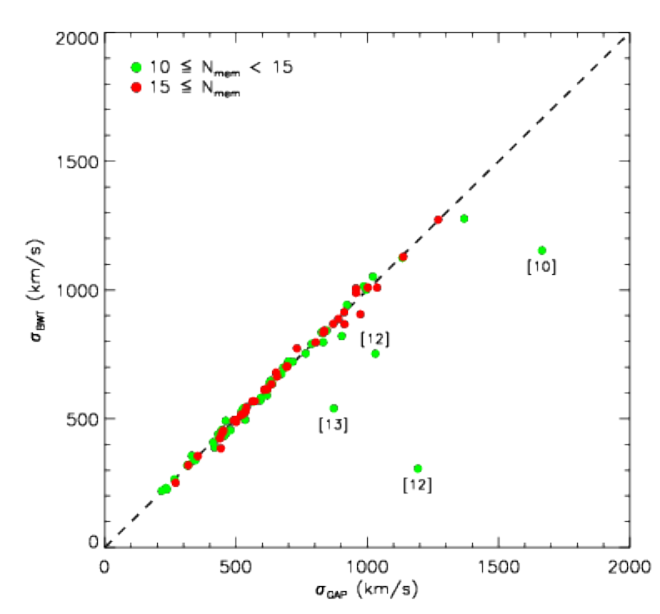
We use two of the most common estimators for the dispersion of velocities, namely the ”gapper” () and the ”bi-weight variance” (). We refer to Beers, Flynn, & Gebhardt (1990) for details in their computation and the algorithm44 4 We used a Fortan version of ROSTAT adapted to our purposes. used for these calculations. We refer the reader to Ruel et al. (2014) for a discussion of measurements of velocity dispersions in the regime of low number of spectroscopic members, in the context of galaxy clusters selected by Sunyaev-Zeldovich effect in the South Pole Telescope data. Both estimators are computed for each cluster, although it is clear that a high enough number of members must enter the derivation to ensure robust measurements. Fig. 21 demonstrates the good agreement between the two measurements provided that . While the majority of clusters also lie on the one-to-one line in this figure, a number of them stand as outliers, possibly impacted by the presence of interlopers or substructures in their list of spectroscopic members.
Evaluating the uncertainties and biases linked to cluster velocity dispersion measurements performed with a small number of spectroscopic members is a rather complex task. It requires in particular an understanding of the selection and sampling processes leading to the list of members entering the catalogue. Ideally, one would want to design end-to-end simulations reproducing all of the steps described above, from the cluster selection in X-rays down to the calculation of velocity dispersions. Such procedures are feasible, for instance by combining N-body simulations and semi-analytical models (Biviano et al., 2006; Saro et al., 2013, e.g.). An alternative, simpler, approach consists in resampling dense observations of clusters with high numbers of spectroscopic members and well-determined velocity dispersions , ensuring the target sampling reproduces that of SPIDERS. We follow this approach in the present work, bearing in mind the opportunities for further, more detailed developments. We resample the observations of the HIFLUGCS sample of clusters (Zhang et al., 2011), imposing a limiting magnitude and a minimal fiber distance corresponding to SPIDERS observations and accounting for the mass and redshift distribution of clusters in SPIDERS. The corresponding procedure is fully described in Zhang et al. (2016). It leads for each HIFLUGCS cluster to 500 resampled realizations, each realization leads in turn to an estimate of an observed . Grouping results by the number of members remaining after resampling, we derive the average value and the spread in . This calculation provides therefore a baseline for the bias-correction and 1- uncertainty on individual velocity dispersion measurements. We note that the catalog of the galaxy redshifts of the HIFLUGCS is a rather clean member galaxy input catalogue, likely almost free from interlopers. Uncertainties derived from the scatter in the down-sampling thus do not account for the effect of interlopers.
4.6 Catalogue production
The updated, accurate, cluster spectroscopic redshifts enter as input of a new computation of X-ray cluster properties.
For the CODEX subsample, this procedure follows the same route as when starting from photometric redshifts (). Details on the procedure can be found in Mirkazemi et al. (2015): assuming a cosmological model, ROSAT fluxes are converted into rest-frame keV luminosities and scaling relations allow an estimate of the cluster mass and typical radius and . The typical uncertainty on the luminosities of CODEX clusters amounts to %, as computed from the Poissonian fluctuation of number counts in ROSAT data. As an illustration, Fig. 4 highlights the position of the SEQUELS-DR12 confirmed clusters in the luminosity-redshift plot, along with the corresponding error bars.
The XCLASS galaxy clusters benefit from high-quality X-ray data, thanks to the exquisite spatial and spectral resolution of XMM: the angular point-spread function FWHM is around , depending on the off-axis angle of the cluster, and the spectral line spread function FWHM is around 100 eV at 1 keV energy. X-ray surface-brightness profiles and spectra are therefore the primary observables from which cluster physical properties are derived. In addition to accurate bolometric luminosities, surface brightness-averaged temperatures of C1 clusters can be measured with relatively good accuracy (%), depending on the actual cluster temperature, the number of counts collected by the instruments and the uncertainties in background subtraction (Clerc et al., 2014, e.g.).
The eROSITA data will be similar to the XMM data, although with a spatial resolution times lower. The methodology to compute X-ray cluster properties by combining SPIDERS spectroscopic redshifts and eROSITA data is expected to lie between that of XCLASS clusters and CODEX clusters.
5 Results from SEQUELS-DR12 sample
Throughout this paper we illustrated the SPIDERS targeting strategy and plans for data analysis by means of the SEQUELS-DR12 pilot sample. We now elaborate on the use of such a sample of spectroscopically confirmed clusters, and present possible science applications with the perspective of the much larger, upcoming, SPIDERS sample.
5.1 Catalogue presentation
5.1.1 The SPIDERS-CODEX clusters
The SEQUELS-DR12 sample consists of 230 validated CODEX systems, out of an initial set of 351 CODEX candidate clusters within the SEQUELS footprint (Alam et al., 2015). Among those 230 clusters, 137 are fully observed within SEQUELS-DR12 (i.e. all tiled targets have received a fiber). Let alone differences in target selection outlined in Sect. 3, this subsample offers a representative view of the expected, times larger, entire SPIDERS sample of clusters. Half of the validated clusters have more than 7 spectroscopic members (8 for completed clusters), this number increases with decreasing redshift, as shown in Fig. 23. Fig. 22 illustrates the X-ray sensitivity of the CODEX survey integrated over the footprint of the area considered for the present catalogue. The median sensitivity in the [0.5-2] keV band is ergs s-1 cm-2.

The redshift distribution of clusters in bins of is shown in Fig. 19 and peaks at . A deficit is observed in one bin around , which we attribute to a mixture of selection effects involving different redshift dependencies of the X-ray sensitivity and RedMapper efficiency, to the preliminary existence of numerous redshifts in SDSS pre-SPIDERS data peaking below and above , and to sample variance.
The X-ray properties of the 230 validated clusters were computed according to the updated redshift value, starting from the ROSAT counts (Mirkazemi et al., 2015, e.g.). Their distribution is displayed in Figure 4. A caveat in the computation of X-ray properties relates to the 10 clusters split into two components after visual inspection. Only one X-ray detection is associated to the original CODEX candidate, and current data do not allow to assign a flux to each of the components. In this work we considered only the primary component as the source of the X-ray emission and therefore discarded the 10 secondary components from the catalogue.
Two points in Fig. 4 are labelled with ’(C)’, indicating likely contamination of the X-ray measurement by a (possibly unrelated) point-source in RASS data. These clusters are optically poor (), hence are among the less reliable sources in the CODEX sample. This class of sources is not targeted in the main SPIDERS program.

5.1.2 The SPIDERS-XCLASS clusters
The SEQUELS-DR12 sample contains three XCLASS-RedMapper clusters, as listed in Table 3, two being completely observed, ID-5117 still awaiting completion. One of the clusters (ID 157) is also found in the CODEX subsample. However, the higher quality of the X-ray data allows to measure its flux, luminosity and temperature with much greater accuracy than the RASS does. This system is in fact better known as Abell 851 (Table 7). The SPIDERS redshift, luminosity and values agree with those found in the literature (Piffaretti et al., 2011). Our XMM-derived gas temperature is similar to the value of keV reported in Mahdavi et al. (2013). Our velocity dispersion estimate computed from 18 SPIDERS spectroscopic members is in agreement with the value of km/s derived by Girardi & Mezzetti (2001) using 55 members; and with that of Oemler et al. (2009), km/s, using 101 members.
After masking point sources, XMM MOS1, MOS2 and PN spectra were extracted in the keV energy range and analysed with XSpec (Arnaud, 1996). An APEC model was fit to measure the cluster temperatures , fixing the element abundance to . The results shown in Table 3 involve a scaling relation linking and (Sun et al., 2009), found by iteratively recomputing the temperature within the aperture. Fluxes were extracted on keV XMM images following a growth curve analysis (Reiprich & Böhringer, 2002; Šuhada et al., 2012; Clerc et al., 2014; Pacaud et al., 2016) and converted into rest-frame keV luminosities assuming the best-fit APEC spectral model found earlier.
This analysis, summarized in Table 3, illustrates the gain in information brought by the XCLASS subsample of SPIDERS clusters (originating from XMM data) in comparison with the CODEX subsample (originating from the shallower RASS data). For instance, the CODEX keV luminosity relative uncertainty on ID 157 is , while the XCLASS one is only a few percent. However, given the low number of XCLASS clusters within the SEQUELS-DR12 demonstration sample, we do not consider them further and defer the interpretation of the full SPIDERS/XCLASS sample to a future study.
| RM | XC | R.A. | Dec | |||||||
| ID | ID | (J2000) | (J2000) | km/s | ( ergs/s/cm2) | ( ergs/s) | (keV) | (Mpc) | ||
| 5117 | 1288 | 122.586 | 48.347 | 11 | 0.84 | |||||
| 157∗ | 1678 | 145.754 | 46.992 | 18 | 0.93 | |||||
| 15756 | 1451 | 170.746 | 46.988 | 6 | - | 0.67 |
5.1.3 The pilot sample catalogue
We provide in Table 4 a condensed summary of the samples and catalogues discussed in this paper.
The list of 230 SPIDERS/CODEX clusters is available online55 5 https://data.sdss.org/sas/dr13/eboss/spiders/analysis/catCluster-SPIDERS_RASS_CLUS-v1.0.fits. The content of the columns in the catalogue are summarized in Table 5. Column names starting with SCREEN result from visual inspection of the system. The luminosity and cluster radius are computed according to the cluster redshift assigned after visual inspection. Note the presence of 10 additional entries in this catalogue, flagged with COMPONENT set to 2, corresponding to putative groups along the line of sight of a given cluster.
| Area: | BOSS imaging | SEQUELS-DR12 | ||
|---|---|---|---|---|
| cand. | val. | cand. | val. | |
| SPIDERS/CODEX | 10 415 | - | 351 | 230 |
| SPIDERS/XCLASS | 278 | - | 7 | 3 |
| MCXC | - | 718 | - | 24 |
| Column | Unit | Description | Example |
| CLUS_ID | SPIDERS/CODEX identification number | 1_4601 | |
| COMPONENT | Component index of the system | 1 | |
| RA | deg | CODEX X-ray detection right ascension (J2000) | 185.497 |
| DEC | deg | CODEX X-ray detection declination (J2000) | 45.310 |
| RA_OPT | deg | CODEX optical detection right ascension (J2000) | 185.522 |
| DEC_OPT | deg | CODEX optical detection declination (J2000) | 45.404 |
| LAMBDA_CHISQ_OPT | Richness () of the CODEX optical detection | 47.2 | |
| Z_LAMBDA | Photometric redshift () of the CODEX optical detection | 0.266 | |
| Z_LAMBDA_ERR | Uncertainty on Z_LAMBDA | 0.009 | |
| NMEM | Number of objects in the CODEX red sequence () | 64 | |
| NOKZ | Number of red-sequence members with a spectroscopic redshift | 21 | |
| SCREEN_CLUZSPEC | Galaxy cluster redshift | 0.2630 | |
| SCREEN_CLUZSPECBOOT | Bootstrap uncertainty on SCREEN_CLUZSPEC | 0.0009 | |
| SCREEN_CLUVDISP_GAP | km/s | Gapper estimate of the cluster velocity dispersion | 869.8 |
| SCREEN_CLUVDISP_BWT | km/s | Square root of the biweight variance velocity dispersion | 868.0 |
| SCREEN_CLUVDISPTYPE | Type of the ”best” velocity dispersion (gapper or bi-weight) | SIG-BWT | |
| SCREEN_CLUVDISPBEST | km/s | Value of the ”best velocity dispersion” | 868.0 |
| SCREEN_DAZSPEC | Mpc | Angular diameter distance computed at SCREEN_CLUZSPEC | 836.9 |
| SCREEN_NMEMBERS | Number of red-sequence members retained as cluster members | 20 | |
| SCREEN_STATUS | Validation status of the cluster assigned by the visual inspector | validated | |
| LX0124 | ergs/s | Luminosity in the rest-frame 0.1-2.4 keV band in | |
| ELX | ergs/s | Uncertainty on LX0124 | |
| R200C_DEG | deg | Apparent radius of the galaxy cluster | 0.093 |
| FLUX052 | ergs/s/cm2 | Galaxy cluster X-ray flux in the 0.5-2.0 keV band | |
| EFLUX052 | ergs/s/cm2 | Uncertainty on FLUX052 | |
| MCXC | Identifier in the MCXC catalogue (Piffaretti et al., 2011), if present | n/a | |
| ANAME | Alternative name in Piffaretti et al. (2011), if present | n/a |
5.2 Cluster relation from individual measurements
Fig. 24 shows the distribution of SPIDERS/CODEX clusters in the - plane, where is computed using the biweight sample variance estimate. Only 39 clusters with more than 15 spectroscopic members are considered here. The raw was corrected from its expected bias, according to the model described in Sect. 4.5. This model is also used to assign error bars to the velocity dispersion measurements, based on the number of members within each system.
Fig. 24 also shows the scaling relation derived from the HIFLUGCS cluster sample. This relation was derived from observations of 62 low-redshift clusters, with much denser spectroscopic coverage (Zhang et al., 2011) than the current SPIDERS sample. For this comparison we considered the core-included luminosity-velocity dispersion relation. Considering the intrinsic scatter residing in the relation (dotted lines in the figure), there is a satisfactory agreement between the position of these points and the HIFLUGCS scaling relations.
We computed the best-fit power-law using the BCES bissector method66 6 We are thankful to C. Sifón for making the Python implementation of the BCES algorithm available at http://home.strw.leidenuniv.nl/˜sifon/pycorner/bces/. (Akritas & Bershady, 1996), as a rough indicator of the overall trend in our sample. For this exercise, we fitted constants and , defined such as:
| (3) |
The consistency between the best-fit power-law and our reference HIFLUGCS relation is encouraging. Proper derivation of scaling relations between X-ray quantities and velocity dispersions relying on a fully consistent statistical treatment and including covariances and selection effects, will constitute a major task once the SPIDERS sample of clusters grows up in size.

5.3 Cluster relation from stacked velocity-distance diagrams
In this section, we investigate how stacking together clusters of similar properties can enhance the statistical power in determining scaling relations between those properties and average velocity dispersion measurements. This method is used (Carlberg, Yee, & Ellingson, 1997; Biviano & Poggianti, 2009; Rines et al., 2013; Munari et al., 2013, e.g.) when the number of spectroscopic members per cluster is low and does not allow accurate, individual, velocity dispersion measurements. Becker et al. (2007) in particular could measure with accuracy the relation between optical richness and velocity dispersion of optically selected galaxy clusters up to by means of stacking systems in richness and redshift. Our approach here is similar and uses X-ray luminosity instead of richness.
5.3.1 An adaptive space binning
We first selected the 108 clusters with at least 8 members. This threshold ensures the uncertainty on the cluster rest velocity to be km/s for a typical 500 km/s velocity dispersion cluster (Eq. 1). We split the sample in 3 redshift slices, namely , and . Each of them is subdivided into a number of bins, according to an adaptive procedure. Starting from the highest luminosity, each bin is enlarged until the clusters it contains bring galaxies within km s-1 of their own cluster rest velocity, and we ensure the size of a bin in luminosity exceeds . This value is indeed comparable to the typical uncertainty in a CODEX cluster luminosity (see Sect. 4.6). An additional constraint was added to the adaptive binning algorithm, such that each bin contains at least 50 % of the number of galaxies expected77 7 was estimated from Rykoff et al. (2012, their Eq. 29). to pertain to a single cluster at the centre bin luminosity. This last requirement ensures that each ”stacked” cluster contains a high enough number of galaxies, thus avoiding biases in the resulting velocity dispersions (see e.g. Zhang et al., 2011, their Fig. 12).
Considering all clusters within a bin, red-sequence members with a spectroscopic redshift were assembled into phase-space diagrams, as shown in Fig. 25 for the specific bin and . In this particular example, 14 clusters are stacked together and 220 spectroscopic galaxies contribute to the stack (corresponding to the black crosses). To produce such stacked diagrams, the projected distance of each member is scaled by of its host cluster, as estimated from the X-ray data88 8 Following the scheme described in Sect. 4.6, this involves a scaling relation .. The cluster centre was chosen to be the optical centre, as derived by the RedMapper algorithm for each CODEX cluster. Individual galaxy velocities were rescaled by their parent cluster so to provide normalized velocities .
Finally, each stack is assigned a typical X-ray luminosity and a representative by taking the error-weighted averages of the luminosities and values of all clusters in the stack.

| Membership method: | Iterative clipping | Caustic | clipping | |||||||||
| ID | ||||||||||||
| (km/s) | (km/s) | (km/s) | ||||||||||
| 1 | 0.03 | 0.26 | 0.02 | 0.2 | 10 | 131 | 123 | 120 | 123 | |||
| 2 | 0.03 | 0.26 | 0.2 | 0.3 | 12 | 188 | 171 | 162 | 171 | |||
| 4 | 0.03 | 0.26 | 0.3 | 0.45 | 15 | 218 | 206 | 196 | 206 | |||
| 5 | 0.03 | 0.26 | 0.45 | 0.75 | 12 | 156 | 145 | 143 | 145 | |||
| 6 | 0.03 | 0.26 | 0.75 | 1.1 | 14 | 220 | 202 | 201 | 205 | |||
| 0 | 0.03 | 0.26 | 1.1 | 2 | 12 | 182 | 171 | 159 | 171 | |||
| 3 | 0.03 | 0.26 | 2 | 20 | 7 | 116 | 114 | 108 | 114 | |||
| 8 | 0.26 | 0.50 | 0.09 | 0.92 | 2 | 16 | 15 | - | - | 16 | ||
| 9 | 0.26 | 0.50 | 0.92 | 2 | 14 | 172 | 161 | 134 | 164 | |||
| 7 | 0.26 | 0.50 | 2 | 20 | 8 | 97 | 96 | 72 | 95 | |||
| 10 | 0.50 | 0.73 | 2 | 20 | 2 | 39 | 23 | 12 | 23 | |||
5.3.2 Member identification in stacked diagrams
Although stacked diagrams are pre-filtered such as to contain only red-sequence members within km/s of their cluster parent, they still contain a fraction of potential interlopers. We investigate three methods to clean stacked diagrams and converge to more precise membership, within the limitations of our present catalogue:
- 1.
The first method is very similar to the one used precedently for individual cluster velocity dispersions. It relies on an iterative 3- clipping technique using the bi-weight average and bi-weight variance as estimates of the centre and velocity dispersions of the stacked clusters. Only members at are considered in this analysis.
- 2.
The second method relies on the identification of the caustic (Diaferio, 1999) in each diagram, similarly implemented as in Zhang et al. (2011). The caustic is a characteristic shape in the phase-space diagrams, it isolates interlopers from virialized members in a cluster. It effectively makes full use of the two-dimensional structure of the diagrams.
- 3.
The third method starts by estimating the expected velocity dispersion of a galaxy cluster of luminosity using Zhang et al. (2011) scaling relations. Galaxies with offset velocities larger than are excluded.
Results are illustrated in Fig. 25, where 202/220, 201/220 and 205/220 members were selected by each of the respective methods, the most stringent selection originating from the caustic identification.
5.3.3 Velocity dispersions from stacked diagrams
Considering only members identified by one of the 3 ’cleaning’ methods, two numerical estimators of the velocity dispersion and their respective uncertainties are derived. In both cases only members within a projected radius less than enter the computation.
The first method computes the bi-weight variance of the selected members, and the uncertainty is based on 1000 bootstrap resamplings of the data.
The second method is similar to Rozo et al. (2015). It is based on maximizing the likelihood:
| (4) |
with the velocities of individual members, the Gaussian function of mean and standard deviation . Here is the maximal velocity, i.e. , and for each of the cleaning method (i), (ii) and (iii) respectively. The parameters and that maximize are found using the Amoeba algorithm and 1000 bootstrap resamplings are performed to estimate the uncertainty on .
Combining the three ’cleaning’ methods to the two estimators leads to 6 estimates of the velocity dispersion for a given stacked phase-space diagram.
5.3.4 The relation of stacked SPIDERS clusters
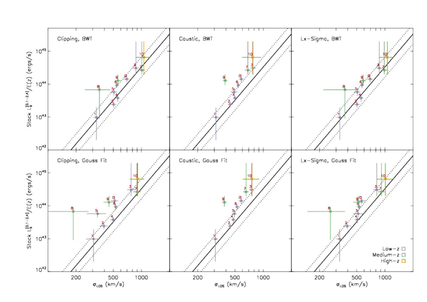
The values of the velocity dispersion in each bin are reported in Fig. 26 (bin numbering listed in Table 6). The externally derived scaling relation superimposed to guide the eye is taken from Zhang et al. (2011) who fit the relation on individual, bright, X-ray clusters in the HIFLUGCS sample. This relation is the same as the black solid line in Fig. 24. The dotted lines represent the typical intrinsic scatter ( dex) in this relation.
We defer quantitative measurements and a thorough assessment of the stacked relation to further studies, that will rely on the entire SPIDERS sample of galaxy clusters and detailed treatment of numerical simulations. We note at this stage a broad agreement between the location of the data points and our reference relation. Our results differ according to the combination of cleaning and fitting method employed. The clipping-based method may lead to more complete but less clean member sampling, the prior-based method is very similar and possibly introduces auto-correlation to some extent.
In the present work, the caustic method filters out more members than the clipping- and prior-based techniques do, and it provides lower velocity dispersion values, hence higher deviations from the fiducial scaling relation (central column in Fig. 24). Simulations (Serra & Diaferio, 2013, e.g.) indicate that the caustic method better distinguishes cluster members from interlopers than other methods ; however, small number statistics impact the precision of the determination of the amplitude of the caustic and thus the caustic mass distribution. A lower number of members tends to provide a slightly reduced amplitude, which causes underestimation of the total mass. Moreover, since the caustic-based filtering makes full use of the projected radius information enclosed in phase-space diagrams, one expects an increased sensitivity of this method to centering uncertainties, to uncertainties in the computation of the normalizing and to sparsity in the 2-dimensional diagrams. Further studies based on numerical simulations tailored to SPIDERS stacks will assess the absolute and relative performances of the methods when combining higher-quality X-ray data (eROSITA data) to the entire, larger, SPIDERS dataset.
Interestingly, data points corresponding to the ’medium-redshift’ bin () deviate from this relation at low- values, and do so more strongly than ’low-redshift’ data points. Part of this deviation can be attributed to sample selection effects and Eddington bias. In App. C we describe a modeling of X-ray selection biases and their impact on scaling relations, by comparing the measured cluster luminosity. As shown in Fig. 31, Eddington bias makes low-mass system (equivalently, low-velocity dispersion systems) appear more luminous on average, and the effect increases with redshift, in agreement with the trend seen in this analysis. The results shown in App. C assume perfect association of the optical spectra to the X-ray emitting intra-cluster gas. Studying the reliability of such identification, as well as possible contaminants to the X-ray (due for instance to the increased presence of X-ray AGN in group-like halos) and optical signals, is beyond the scope of this paper. These additional sources of bias, likely to dominate in the low-count/low-richness regime, need to be addressed with further simulations.
6 Comparison with previous X-ray cluster catalogues

We compare our work to the objects extracted from the MCXC compilation of catalogues (Piffaretti et al., 2011), which contains most of the ROSAT-based samples, including serendipitous detections from deep pointed observations. Fig. 27 shows the distribution on sky of the samples discussed in this paper. We find 18 matches between the SPIDERS pilot sample and the MCXC database within 3 arcmin of the CODEX X-ray position. Their properties are summarized in Table 7 and compared with values extracted from the MCXC compilation. Five systems exhibit a richness lower than 20 in the overlap between the two catalogues. Fig. 28 compares the redshift values in both catalogues and demonstrates their good agreement. All but two agree within 1000 km s-1 of the MCXC redshift, the other two agree within 3000 km s-1.
Within the survey footprint, 6 MCXC clusters could not be matched to a SPIDERS validated cluster (Table. 8). Five of them have values of luminosity and redshift (Fig. 3) consistent with sources below or at the edge of the CODEX X-ray detectability – these are sources detected in deep ROSAT pointed observations (Vikhlinin et al., 1998; Mullis et al., 2003). In particular, MCXC J0921.2+4528 at is the brightest of these five and shows a flux significant at a 1.3- level only (in the ROSAT All-sky survey) at the value of ergs s-1 cm-2, hence it lies in the largely incomplete part of the sensitivity range. The sixth source is Abell 1361 and is located within a masked region of the ROSAT all-sky data used as input of the CODEX X-ray finding algorithm (a degree north of the sensitivity dip visible in Fig. 27 at R.A. 11h40m and Dec. ).

| SPIDERS | MCXC | Alternative | |||||
| ID | ID | name | (SPIDERS) | (MCXC) | (SPIDERS) | (MCXC) | |
| ergs s-1 | ergs s-1 | ||||||
| 1_2952 | J1053.7+4929 | 0.140 | 1.7 | 12.2 | |||
| 1_4189 | J0921.1+4538 | 3C 219 | 0.175 | 1.4 | 13.4 | ||
| 2_2449 | J0907.8+4936 | VV 196 | 0.035 | 0.1 | 17.1 | ||
| 1_2848 | J1013.6+4933 | VMF98 87 | 0.133 | 0.3 | 17.7 | ||
| 1_4021 | J0822.1+4705 | A0646 | 0.130 | 3.0 | 19.0 | ||
| 1_2788 | J1025.0+4750 | A1003 | 0.052 | 0.1 | 24.4 | ||
| 1_4240 | J0958.3+4702 | 0.390 | 1.9 | 28.6 | |||
| 2_4405 | J1351.7+4622 | 0.062 | 0.3 | 31.4 | |||
| 1_1172 | J0759.7+5400 | Zw 0755.8+5408 | 0.103 | 1.1 | 34.9 | ||
| 1_1198 | J0819.9+5634 | VMF98 50 | 0.260 | 0.9 | 37.1 | ||
| 2_3671 | J0804.3+4646 | A0616 | 0.187 | 1.4 | 53.1 | ||
| 2_3682 | J0805.7+4541 | A0620 | 0.135 | 0.9 | 64.3 | ||
| 2_2602 | J1023.6+4907 | A0990 | 0.144 | 3.9 | 72.5 | ||
| 2_4317 | J1313.1+4616 | A1697 | 0.183 | 2.6 | 82.5 | ||
| 1_3111 | J1229.0+4737 | A1550 | 0.254 | 3.3 | 108.4 | ||
| 2_4315 | J1306.9+4633 | A1682 | 0.226 | 5.1 | 123.9 | ||
| 2_3664 | J0825.5+4707 | A0655 | 0.127 | 2.8 | 131.8 | ||
| 1_4241∗ | J0943.1+4659 | A0851 | 0.407 | 4.9 | 148.8 |
| MCXC | Alternative | ||
|---|---|---|---|
| ID | name | (MCXC) | (MCXC) |
| ergs s-1 | |||
| J1143.5+4623 | A1361 | 0.117 | 2.8 |
| J1256.6+4715 | VMF98 129 | 0.404 | 0.5 |
| J0818.9+5654 | VMF98 48 | 0.260 | 0.3 |
| J0820.4+5645 | VMF98 51 | 0.043 | 0.02 |
| J0921.2+4528 | VMF98 70 | 0.315 | 1.0 |
| J1056.2+4933 | VMF98 94 | 0.199 | 0.2 |
7 Conclusions
This paper introduces the SPIDERS spectroscopic follow-up of X-ray galaxy clusters with particular emphasis on the selection of targets. The galaxy cluster component in SDSS-IV/SPIDERS will obtain optical spectra of 40 000-50 000 galaxies identified as potential members of 5 000 to 6 000 massive (from to , peaking at ) X-ray galaxy clusters in the Northern hemisphere, up to redshift 0.6 and above. This massive observational effort will bring the average number of galaxy spectra within their respective red-sequences from 2 to 10, therefore allowing precise calculation of galaxy cluster redshifts, relying on a median number of 8 member galaxies per system. Until the launch of the eROSITA satellite (2017), the observed sample of X-ray galaxy clusters originates from the ROSAT all-sky survey and from XMM-Newton archival observations. The target selection heavily relies on the RedMapper algorithm, that is able to assign membership probabilities to galaxies photometrically identified as red-sequence members across the SDSS imaging data. The eROSITA all-sky survey will complement this preliminary observational tier by bringing denser samples than ROSAT and a more detailed X-ray information over the entire surveyed area.
The achieved spectral quality will allow secure redshift measurements of the targeted red galaxies (up to in aperture), relying particularly on the extensive developments achieved for the BOSS and eBOSS surveys: observation planning and realization, processing pipelines, infrastructure, databases and analysis tools. A number of steps are envisaged to construct reliable catalogues of X-ray validated clusters with redshift, by assigning membership of galaxies within their parent clusters. These procedures will mix automatized algorithms – to treat the bulk of the dataset in a most efficient way – and visual screening – to address peculiar cases, especially in the low-member regime. Throughout this paper, the feasibility of this programme was demonstrated based on a pilot sample of 230 galaxy clusters. All were confirmed with spectroscopic data, providing accurate redshifts at the level. We highlighted the difficulties implied by reduced X-ray information for the poorer systems (projection effects, ambiguous associations, etc.) Better X-ray data are required for these low-mass, high-redshift systems, as already provided by XMM or by eROSITA in the future.
The SPIDERS cluster follow-up programme is essential to achieve the cosmological analysis of the mass function and tridimensional distribution of X-ray galaxy clusters. Indeed, precise redshift information enables precise determination of cluster X-ray properties (luminosity, temperature, gas mass, etc.) related to the host halo mass, and accurate localization of these objects in the cosmic web. Moreover, a wealth of additional science cases will be addressed via the SPIDERS survey. Among them, we have shown that dynamical mass estimates are accessible for a subset of the clusters (in this paper through the radial velocity dispersion proxy), despite the low number of spectroscopic members per individual system. In particular, the stacking of X-ray clusters offers a promising avenue to the study of average properties in such a large sample. Specifically, the results of our pilot study could establish that the radial velocity dispersions correlate with the X-ray luminosity of (stacked) clusters in a similar way as local galaxy clusters do. The methods introduced in this paper are meant to evolve during the course of the survey, most likely including state-of-the art and most recent techniques. The quality and number of galaxy spectra within or in the line-of-sight of galaxy clusters will be exploited to address several science topics, ranging from galaxy formation and evolution to properties of the intergalactic medium.
Finally, besides the exceptional dataset provided by the programme and its predicted science outcome, SPIDERS is already starting to pave the way for future, large-area, spectroscopic surveys. In particular, the 4MOST instrument on the ESO-VISTA telescope (de Jong et al., 2014) will follow-up eROSITA clusters in the Southern hemisphere in the early 2020s and will largely benefit from the science and technical developments pursued within SPIDERS in SDSS-IV.
Acknowledgments
We thank the referee for useful discussion that helped in improving the content of this paper.
Funding for the Sloan Digital Sky Survey IV has been provided by the Alfred P. Sloan Foundation, the U.S. Department of Energy Office of Science, and the Participating Institutions. SDSS-IV acknowledges support and resources from the Center for High-Performance Computing at the University of Utah. The SDSS web site is www.sdss.org.
SDSS-IV is managed by the Astrophysical Research Consortium for the Participating Institutions of the SDSS Collaboration including the Brazilian Participation Group, the Carnegie Institution for Science, Carnegie Mellon University, the Chilean Participation Group, the French Participation Group, Harvard-Smithsonian Center for Astrophysics, Instituto de Astrofísica de Canarias, The Johns Hopkins University, Kavli Institute for the Physics and Mathematics of the Universe (IPMU) / University of Tokyo, Lawrence Berkeley National Laboratory, Leibniz Institut für Astrophysik Potsdam (AIP), Max-Planck-Institut für Astronomie (MPIA Heidelberg), Max-Planck-Institut für Astrophysik (MPA Garching), Max-Planck-Institut für Extraterrestrische Physik (MPE), National Astronomical Observatory of China, New Mexico State University, New York University, University of Notre Dame, Observatário Nacional / MCTI, The Ohio State University, Pennsylvania State University, Shanghai Astronomical Observatory, United Kingdom Participation Group, Universidad Nacional Autónoma de México, University of Arizona, University of Colorado Boulder, University of Oxford, University of Portsmouth, University of Utah, University of Virginia, University of Washington, University of Wisconsin, Vanderbilt University, and Yale University.
Y.Y.Z acknowledges support by the German BMWI through the Verbundforschung under grant 50 OR 1506.
Funding for SDSS-III has been provided by the Alfred P. Sloan Foundation, the Participating Institutions, the National Science Foundation, and the U.S. Department of Energy Office of Science. The SDSS-III web site is http://www.sdss3.org/.
References
- Adami et al. (2011) Adami C., et al., 2011, A&A, 526, A18
- Akritas & Bershady (1996) Akritas M. G., Bershady M. A., 1996, ApJ, 470, 706
- Alam et al. (2015) Alam S., et al., 2015, ApJS, 219, 12
- Allevato et al. (2012) Allevato V., et al., 2012, ApJ, 758, 47
- Arnaud (1996) Arnaud K. A., 1996, ASPC, 101, 17
- Bahcall & Cen (1993) Bahcall N. A., Cen R., 1993, ApJ, 407, L49
- Becker et al. (2007) Becker M. R., et al., 2007, ApJ, 669, 905
- Beers, Flynn, & Gebhardt (1990) Beers T. C., Flynn K., Gebhardt K., 1990, AJ,100, 32
- Bernardi et al. (2007) Bernardi M., Hyde J. B., Sheth R. K., Miller C. J., Nichol R. C., 2007, AJ, 133, 1741
- Biviano et al. (2006) Biviano A., Murante G., Borgani S., Diaferio A., Dolag K., Girardi M., 2006, A&A, 456, 23
- Biviano & Poggianti (2009) Biviano A., Poggianti B. M., 2009, A&A,501, 419
- Blanton et al. (2017) Blanton, M.R., et al. 2017, AJ, submitted
- Böhringer et al. (2004) Böhringer H., et al., 2004, A&A, 425, 367
- Bolton et al. (2012) Bolton A. S., et al., 2012, AJ, 144, 144
- Borm et al. (2014) Borm K., Reiprich T. H., Mohammed I., Lovisari L., 2014, A&A, 567, A65
- Burenin et al. (2007) Burenin R. A., Vikhlinin A., Hornstrup A., Ebeling H., Quintana H., Mescheryakov A., 2007, ApJS, 172, 561
- Burke et al. (2003) Burke D. J., Collins C. A., Sharples R. M., Romer A. K., Nichol R. C., 2003, MNRAS, 341, 1093
- Carlberg, Yee, & Ellingson (1997) Carlberg R. G., Yee H. K. C., Ellingson E., 1997, ApJ, 478, 462
- Clerc et al. (2012) Clerc N., Sadibekova T., Pierre M., Pacaud F., Le Fèvre J.-P., Adami C., Altieri B., Valtchanov I., 2012, MNRAS, 423, 3561
- Clerc et al. (2014) Clerc N., et al., 2014, MNRAS, 444, 2723
- Danese, de Zotti, & di Tullio (1980) Danese L., de Zotti G., di Tullio G.,1980, A&A, 82, 322
- Dawson et al. (2016) Dawson K. S., et al., 2016, AJ, 151, 44
- Diaferio (1999) Diaferio A., 1999, MNRAS, 309, 610
- Ebeling et al. (2000) Ebeling H., Edge A. C., Allen S. W., Crawford C. S., Fabian A. C., Huchra J. P., 2000, MNRAS, 318, 333
- Ebrero et al. (2009) Ebrero J., et al., 2009, A&A, 493, 55
- Finoguenov et al. (2010) Finoguenov A., et al., 2010, MNRAS, 403, 2063
- Girardi & Mezzetti (2001) Girardi M., Mezzetti M., 2001, ApJ, 548, 79
- Gladders & Yee (2000) Gladders M. D., Yee H. K. C., 2000, AJ, 120,2148
- Gunn et al. (2006) Gunn J. E., et al., 2006, AJ, 131, 2332
- Guzzo et al. (2009) Guzzo L., et al., 2009, A&A, 499, 357
- Hansen et al. (2009) Hansen S. M., Sheldon E. S., Wechsler R. H., Koester B. P., 2009, ApJ, 699, 1333
- Henry & Arnaud (1991) Henry J. P., Arnaud K. A., 1991, ApJ, 372,410
- Ikebe et al. (2002) Ikebe Y., Reiprich T. H., Böhringer H., Tanaka Y., Kitayama T., 2002, A&A, 383, 773
- Jones & Forman (1984) Jones C., Forman W., 1984, ApJ, 276, 38
- de Jong et al. (2014) de Jong, R. S., Barden, S., Bellido-Tirado, O., et al. 2014, Proc. SPIE, 9147, 91470M
- Mahdavi et al. (2013) Mahdavi A., Hoekstra H., Babul A., Bildfell C., Jeltema T., Henry J. P., 2013, ApJ, 767, 116
- Mantz et al. (2010) Mantz A., Allen S. W., Rapetti D., Ebeling H., 2010, MNRAS, 406, 1759
- Maraston et al. (2009) Maraston C., Strömbäck G., Thomas D., Wake D. A., Nichol R. C., 2009, MNRAS, 394, L107
- Martini et al. (2013) Martini P., et al., 2013, ApJ, 768, 1
- Menzel et al. (2016) Menzel M.-L., et al., 2016, MNRAS, 457, 110
- Merloni et al. (2012) Merloni A., et al., 2012, arXiv, arXiv:1209.3114
- Mirkazemi et al. (2015) Mirkazemi M., et al., 2015, ApJ, 799, 60
- Mullis et al. (2003) Mullis, C. R., McNamara, B. R., Quintana, H., et al. 2003, ApJ, 594, 154
- Munari et al. (2013) Munari E., Biviano A., Borgani S., Murante G., Fabjan D., 2013, MNRAS, 430, 2638
- Oemler et al. (2009) Oemler A., Jr., Dressler A., Kelson D., Rigby J., Poggianti B. M., Fritz J., Morrison G., Smail I., 2009, ApJ, 693, 152-173
- Pacaud et al. (2006) Pacaud F., et al., 2006, MNRAS, 372, 578
- Pacaud et al. (2016) Pacaud F., et al., 2016, A&A, 592, A2
- Pierre et al. (2016) Pierre M., et al., 2016, A&A, 592, A1
- Piffaretti et al. (2011) Piffaretti R., Arnaud M., Pratt G. W., Pointecouteau E., Melin J.-B., 2011, A&A, 534, A109
- Predehl et al. (2014) Predehl P., et al., 2014, SPIE, 9144, 91441T
- Popesso et al. (2005) Popesso P., Böhringer H., Romaniello M., Voges W., 2005, A&A, 433, 415
- Reiprich & Böhringer (2002) Reiprich T. H., Böhringer H., 2002, ApJ, 567, 716
- Rines et al. (2013) Rines K., Geller M. J., Diaferio A., Kurtz M. J., 2013, ApJ, 767, 15
- Romer et al. (2000) Romer A. K., et al., 2000, ApJS, 126, 209
- Rosati et al. (1998) Rosati P., Della Ceca R., Norman C., Giacconi R., 1998, ApJ, 492, L21
- Rozo et al. (2015) Rozo E., Rykoff E. S., Becker M., Reddick R. M., Wechsler R. H., 2015, MNRAS, 453, 38
- Ruel et al. (2014) Ruel J., et al., 2014, ApJ, 792, 45
- Rykoff et al. (2012) Rykoff E. S., et al., 2012, ApJ, 746, 178
- Rykoff et al. (2014) Rykoff E. S., et al., 2014, ApJ, 785, 104
- Sadibekova et al. (2014) Sadibekova T., Pierre M., Clerc N., Faccioli L., Gastaud R., Le Fevre J.-P., Rozo E., Rykoff E., 2014, A&A, 571, A87
- Saro et al. (2013) Saro A., Mohr J. J., Bazin G., Dolag K., 2013, ApJ, 772, 47
- Schuecker et al. (2003) Schuecker P., Böhringer H., Collins C. A.,Guzzo L., 2003, A&A, 398, 867
- Serra & Diaferio (2013) Serra A. L., Diaferio A., 2013, ApJ, 768, 116
- Šuhada et al. (2012) Šuhada R., et al., 2012, A&A, 537, A39
- Sun et al. (2009) Sun M., Voit G. M., Donahue M., Jones C., Forman W., Vikhlinin A., 2009, ApJ, 693, 1142
- Tinker et al. (2008) Tinker J., Kravtsov A. V., Klypin A., Abazajian K., Warren M., Yepes G., Gottlöber S., Holz D. E., 2008, ApJ, 688, 709
- Vikhlinin et al. (1998) Vikhlinin A., McNamara B. R., Forman W., Jones C., Quintana H., Hornstrup A., 1998, ApJ, 502, 558
- Vikhlinin et al. (2009) Vikhlinin A., et al., 2009, ApJ, 692, 1060
- Weinberg et al. (2013) Weinberg D. H., Mortonson M. J., Eisenstein D. J., Hirata C., Riess A. G., Rozo E., 2013, PhR, 530, 87
- Zhang et al. (2011) Zhang Y.-Y., Andernach H., Caretta C. A., Reiprich T. H., Böhringer H., Puchwein E., Sijacki D., Girardi M., 2011, A&A, 526, A105
- Zhang et al. (2016) Zhang Y.-Y., et al., 2016, arXiv, arXiv:1608.06585
Appendix A Impact of a lower priority threshold on the targeting
We presented in Sect. 3.1 our choice to lower the priority threshold in the submitted target list in order to accommodate for the higher density of unique galaxy clusters in certain area of sky. In the particular case of the eboss3 chunk, a threshold of 33 (instead of 80) was set. Fig. 29 shows the impact of this change, resulting in a decrease in the net number of targets per system (from to , see Fig. 9). Fig. 30 shows that targets in the outer regions of clusters are more severely impacted by this incompleteness. This is easily explained by the link between priority and RedMapper probability that in particular accounts for the galaxy’s cluster-centric distances through a radial density profile weighting (Rykoff et al., 2014). As the interloper rate is expected to decrease with decreasing cluster-centric distance (Saro et al., 2013, e.g.), the impact of a lower number of spectroscopic redshifts per cluster should be mitigated by a lower interloper rate.

 |
 |
Appendix B Description of the target catalogue
The target catalogue contains the list of targets submitted to the tiling algorithm. It is made available as part of SDSS Data Release 1399 9 http://www.sdss.org. Nominally, SPIDERS targets galaxies selected within the optical red-sequence of individual galaxy clusters. In the Tier-0 phase of SPIDERS, these clusters are drawn from the CODEX and XCLASS samples.
The targets of SPIDERS clusters are split into three categories:
- •
in the 117 SEQUELS plates (66 of them have already been released as part of SDSS DR12), the SPIDERS_RASS_CLUS target flag corresponds to objects indifferently selected among CODEX or XCLASS red-sequences;
- •
in all eBOSS plates, the SPIDERS_RASS_CLUS target flag corresponds to object selected in CODEX red-sequences;
- •
in all eBOSS plates, the SPIDERS_XCLASS_CLUS target flag corresponds to object selected in X-CLASS red-sequences.
In BOSS and eBOSS, all SEQUELS targets are tracked by the EBOSS_TARGET0 bitmask and the SPIDERS_RASS_CLUS clusters targets correspond to bit 21. In eBOSS, all SPIDERS targets (clusters and AGN) are tracked by the EBOSS_TARGET1 with bit 31. The EBOSS_TARGET_2 bitmask distentangles between the various SPIDERS targets: the SPIDERS_RASS_CLUS targets correspond to bit 1 and SPIDERS_XCLASS_CLUS targets to bit 5.
The SPIDERS clusters target catalogues contain the minimal information necessary for the tiling algorithm, as well as supplementary information relative to their parent galaxy cluster. Table 9 shows a subset of the SPIDERS target catalogue. FIBER2MAG is the aperture magnitude of the source in each of the five SDSS filters. TARGETSELECTED is the confirmation rank of the galaxy in the red-sequence. The cluster photometric redshift (and uncertainty ) and the richness are given together with the internal cluster identifier CLUS_ID. The priority column plays an important role in the tiling algorithm as it defines how fiber collisions are resolved. Note that SPIDERS AGN all have a priority set to 1.
| RA | Dec | FIBER2MAG () | TARGETSELECTED | CLUS_ID | Priority | |||
|---|---|---|---|---|---|---|---|---|
| deg | deg | mag. | ||||||
| 117.9716 | 27.3276 | 1 | 0.265 | 0.019 | 12.5 | 1_10000 | 0 | |
| 112.1157 | 26.6917 | 1 | 0.137 | 0.005 | 30.2 | 1_10008 | 0 | |
| … | … | … | … | … | … | … | … | … |
| 134.8594 | 55.3670 | (23.0, 22.0, 20.6, 20.1, 19.7) | 2 | 0.269 | 0.023 | 11.8 | 1_1284 | 3 |
| … | … | … | … | … | … | … | … | … |
| 201.2000 | 28.4698 | (24.3, 22.3, 20.9, 20.3, 20.1) | 36 | 0.266 | 0.009 | 48.3 | 2_9973 | 79 |
Appendix C Modeling the selection and measurement biases

The SPIDERS/CODEX sample is based on a sample of faint X-ray sources, down to 4 photon counts in RASS data. Measurement of scaling relations and population studies are therefore subject to selection and measurement biases, that can be addressed via simulations. As an illustration, we show in Fig. 31 the outcome of a series of simulations of CODEX clusters. The sensitivity curves were calculated specifically according to the footprint of the pilot sample presented in this paper (see Fig. 27 and Fig. 22). The ’true’ luminosity is that expected from a simple mass-luminosity relation and is not necessarily equal to the quantity measured in real data. Due to Eddington bias and in presence of intrinsic scatter in the mass-luminosity relation, faint objects are on average measured with higher luminosities, hence the upturn at low luminosities. The effect is redshift-dependent and more pronounced for high-redshift objects.
Given that the RASS luminosity might be affected by the AGN, we have included into the calculation of the observed luminosity the effect of unresolved AGN. Our model combines the evolution of AGN X-ray luminosity function of Ebrero et al. (2009) with the halo occupation distribution (HOD) study of Allevato et al. (2012). The resulting mean contamination of AGN per cluster is ergs s-1 in the rest-frame 0.5–2 keV band, which has to be rescaled up self-consistently using cluster K-correction factors of 1.5. This model is in a very good agreement with the results of Martini et al. (2013), who measured AGN activity in clusters at an average level of ergs s-1 in the 0.5–8 keV band. In our highest redshift bin, the model predicts an AGN contribution of erg s-1, which on average is still a subdominant contribution to the observed flux. This model predicts that the and low ( ergs s-1) sample requires significant correction for AGN contamination.
The SPIDERS/XCLASS sample is based on a different selection technique and different X-ray datasets. The galaxy cluster X-ray selection function are presented in Clerc et al. (2012) along with the X-ray flux measurement calibrations.