Hartree potential dependent exchange functional

To start our work, we consider the construction of a proper reduced ingredient that depends on the Hartree potential and has the correct features to be usefully employed in the construction of density functionals. This is the Hartree reduced parameter

This ingredient is invariant under the uniform scaling of the density ($n_{\gamma}(\mathbf{r})=\gamma^{3}n(\gamma\mathbf{r})$, with $\gamma>0$), i.e. it behaves as $\eta^{u}_{\gamma}(\mathbf{r})=\eta^{u}(\gamma\mathbf{r})$. This invariance is a key property for any input ingredient to be used in the development of semilocal DFT functionals. In fact, it is satisfied by all the semilocal ingredients:

where $k_{F}=(3\pi^{2}n)^{1/3}$ is the Fermi wavevector, $\tau^{unif}=\frac{3}{10}(3\pi^{2})^{2/3}n^{5/3}$ is the Thomas-Fermi kinetic energy density [92, 93], and $\tau^{W}=\tau^{unif}5s^{2}/3$ is the von Weizsäcker kinetic energy density [94].

Additional important formal properties of $\eta^{u}$ can be obtained considering its behavior under the coordinate and particle-number density scaling [95] ($n^{(\beta)}_{\gamma}(\mathbf{r})=\gamma^{3\beta+1}n(\gamma^{\beta}\mathbf{r})$, with $\gamma>0$ and $\beta$ being a parameter), which defines a whole family of scaling relations. Under this scaling, we have $\eta^{u}\rightarrow\gamma^{2/3}\eta^{u}$, i.e. the Hartree reduced ingredient scales as $N^{2/3}$, with $N$ being the number of electrons. This result indicates that, unlike the semilocal parameters, $\eta^{u}$ is a size-extensive quantity, increasing with the number of electrons. We note that, in spite of this feature, the reduced Hartree parameter is anyway behaving in a proper size-consistent way as shown in Appendix A.

Moreover, we can note that the scaling properties of $\eta^{u}$ do not depend on the value of the parameter $\beta$. Thus, for the uniform-electron-gas and the Thomas-Fermi scalings [95, 96], where the $\gamma\rightarrow\infty$ limit is important, large values of $\eta^{u}$ are relevant; on the opposite, for the homogeneous and fractional-particle scalings [95, 97, 98], where $\gamma\rightarrow 0$, small values of $\eta^{u}$ are important. These considerations will be significant to analyze the behavior of an $\eta^{u}$-dependent enhancement factor in different conditions.

In Fig. 1, we compare the behavior of $\eta^{u}$ with that of the other semilocal ingredients for some atoms and dimers.

It can be seen that $\eta^{u}$ behaves rather different than the other conventional semilocal reduced parameters ($s$, $z$, and $\alpha$), being in general more shallowed and averaged: $\eta^{u}$ is in fact a non-local ingredient and thus it contains, at every point of space, information on the whole system. Moreover, it is larger than zero at any point in space (unlike $s$, for example); in the density tail asymptotic region we always have

like $s$ but in contrast to $\alpha$ which vanishes for iso-orbital density tails (e.g. for Be).

Thus, $\eta^{u}$ appears to be an interesting tool for the construction of advanced functionals both to complement the information available from standard semilocal reduced ingredient and to add information on the shape of the exchange enhancement factor.

The most important feature of $\eta^{u}$ is that the simple exchange enhancement factor

yields immediately Eqs. (2) and (3) [for the former, note that the exchange energy satisfies the spin-scaling relation [99] $E_{x}[n_{\uparrow},n_{\downarrow}]=(E_{x}[2n_{\uparrow}]+E_{x}[2n_{\downarrow}])/2$]. Hence, $\eta^{u}$ represents the exact exchange enhancement factor for any one- and two-electron system.

Finally, it is also useful to define the bounded ingredient

that is small everywhere for large systems, but also in the tail of the density (where $\eta^{u}\rightarrow\infty$).

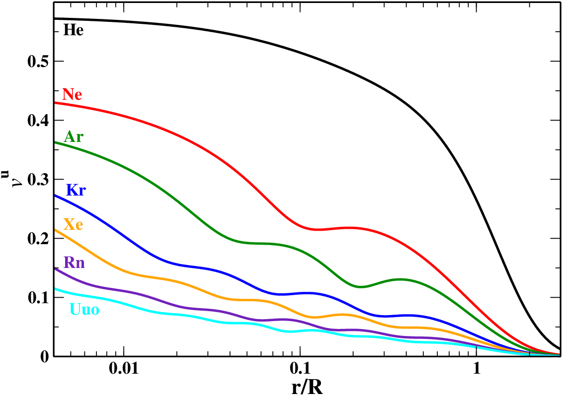
In Fig. 2, we show $\upsilon^{u}$ for the noble atoms of the periodic table. One can see that in most of the space the curves are not intersecting, such that $\upsilon^{u}$ can be considered a good atomic indicator, being of interest for functional development.

In the previous subsection we introduced the Hartree reduced parameter and we showed that it posses interesting properties that suggest its utility as input quantity in the construction of advanced density functionals. On the other hand, we have observed that in general $\eta^{u}$ is always large in magnitude. Thus, the proper use of this quantity in functional development is not trivial and the construction of a good u-meta-GGA functional represents instead a challenge.

To attempt to fulfill this task, we consider the following ansatz for the u-meta-GGA exchange enhancement factor

where

with $\mu^{MGE2}=0.26$ being the coefficient of the modified second-order gradient expansion (MGE2) [96, 101, 30], and the $a_{1}=1/6$, $a_{2}=0.05$, and $a_{3}=0.08$ being non-empirical parameters fitted to a class of four-electron model systems described in Section II.3.

The function $b=b(z)$ controls the transition from pure u-meta-GGA behavior ($F_{x}^{u-MGGA}=\eta^{u}$), which is exact for iso-orbital regions ($z=1$), to a meta-GGA like behavior $(F_{x}^{u-MGGA}=F_{x}^{1}$), which is appropriate for slowly-varying density limit ($z\approx 0$). Moreover, $a_{2}$ is a parameter which helps to tune the value of the second-order coefficient in the Taylor expansion at slowly-varying densities for each atom. This is done using the parameter $\upsilon^{u}$ as an atomic indicator. Note that for small atoms $\mu>\mu^{MGE2}$ (here the gradient expansion is less meaningful, and the results are very sensitive to the functional form) , whereas in the semiclassical limit (with an infinite number of electrons) $\mu=\mu^{MGE2}$. Finally, $a_{3}$ modulates the behavior of the functional in the tail of the density.

The u-meta-GGA exchange functional has been costructed satisying the following properties:

• -

  For one and two electron systems $z=1$, so that $b=\beta=0$, yielding $A=\eta^{u}$ and $F_{X}^{1}=1$, therefore $F_{x}^{u-MGGA}=\eta^{u}$ is exact (see Eq. (11));

• -

  Under the uniform density scaling $n_{\gamma}(\mathbf{r})=\gamma^{3}n(\gamma\mathbf{r})$, with $\gamma>0$, it behaves correctly as $E_{x}^{u-MGGA}[n_{\gamma}]=\gamma E_{x}^{u-MGGA}[n]$;

• -

  It is size-consistent (see Appendix A);

• -

  For many-electron systems, we can distinguish different regions:

  • –

    In the slowly-varying density limit ($s\rightarrow 0$, $z\rightarrow 5s^{2}/3+\mathcal{O}(|\nabla n|^{4})$, $\alpha\rightarrow 1+\mathcal{O}(|\nabla n|^{2})$) we have $b\rightarrow 1$ and $\beta\rightarrow 1$, thus $A\rightarrow 1$ and

    $$F_{x}^{u-MGGA}\rightarrow F_{x}^{1}\rightarrow 1+\mu s^{2}\;.$$

    (19)

    Note that in the limit of large atoms $\mu\rightarrow\mu^{MGE2}$, such that the semiclassical atom theory [96, 12] is correctly recovered.

  • –

    In the density tail asymptotic region with valence orbitals having a non-zero angular momentum quantum number ($s\rightarrow\infty,z<1)$ so that $\beta\rightarrow 0$. We have also that $\eta^{u}\rightarrow\infty$ and $A\rightarrow 1$ (as $\beta^{(1/\eta^{u})}\rightarrow 1$), thus

    $$F_{x}^{u-MGGA}\rightarrow F_{x}^{1}\rightarrow\frac{2\pi\sqrt{\alpha}}{3\sqrt{5}\sqrt{\ln(1+\alpha)}}\ .$$

    (20)

    Equation (20) is an exact meta-GGA constraint for metallic surfaces [39], making asymtotically exact both the exchange energy per particle and the potential, while for finite systems we found (see Appendix B) that the exchange energy per particle decays as $\epsilon_{x}\rightarrow-C/r^{3/2}$, and the exchange potential decays as $v_{x}\rightarrow-C/(2r^{3/2})$, with $C$ being a constant dependent on the angular momentum quantum number of the outer shell, if $\alpha\rightarrow\infty$ [102]. Thus, for finite systems Eq. (20) is not an exact constraint [102, 103]. Nevertheless, this behavior is definitely more realistic than the usual exponential decay behavior of most semilocal functionals. In any case, we underline that the Hartree potential is not used to describe the asymptotic region, in contrast to functionals based on the Fermi-Amaldi potential: instead, the meta-GGA expression in Eq. (20) is used. Moreover, in this work we are only considering non self-consistent results, which are thus quite unaffected by the choice of the functional in the asymptotic region.

We note that the u-meta-GGA enhancement factor diverges for $\eta^{u}\rightarrow+\infty$ and/or $s\rightarrow+\infty$ (i.e. in the tail of the density). Therefore, unlike other functionals, it does not respect the local form of the Lieb-Oxford bound [104, 105, 106]. We note that this feature is anyway not an exact constraint and it is indeed also strongly violated by the conventional exact exchange energy density [107]. However, we recall that the global Lieb-Oxford bound, which is the true exact condition, is not tight, being usually fulfilled for all known physical systems, by most of the functionals [108]. As shown in the next section, the u-meta-GGA functional is accurate for atoms and molecules. Thus, it implicitly satisfies the Lieb-Oxford bound for these systems.

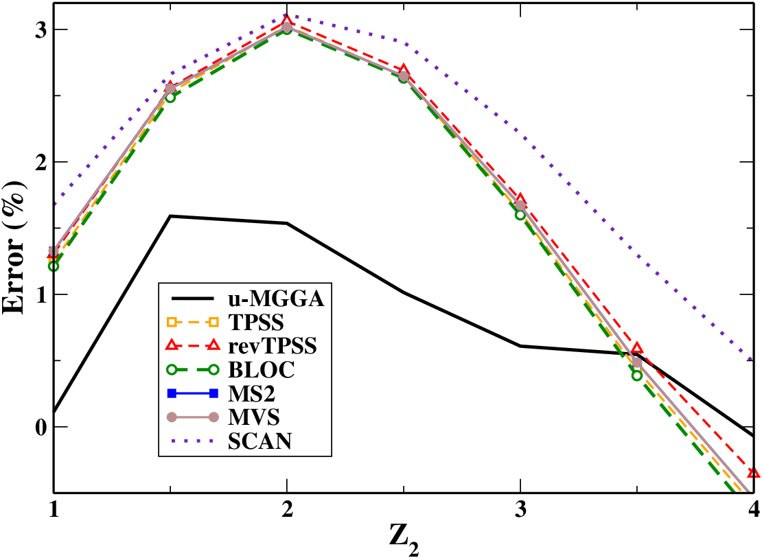
Because the u-meta-GGA is exact for any one- and two-electron systems, we require it to be as accurate as possible also for four-electron systems. To this purpose, we consider the four-electron hydrogenic-orbital model ($1s^{2}2s^{2}$), with the following one-electron wavefunctions ($\psi_{nlm}$ with $n$, $l$, and $m$ being the principal, the angular, and the azimuthal quantum numbers respectively)

with $Z_{1}$ and $Z_{2}$ being the nuclear charges seen by the $1s$ and $2s$ electrons, respectively. Note that for the real beryllium atom, $Z_{1}\approx 4$, and $Z_{2}\approx 2$. This model system is analytical and simple, and can cover important physics by varying $Z_{1}$ and $Z_{2}$. In Appendix C we show in detail the case $Z_{1}=Z_{2}=Z$. We also recall that the hydrogenic orbitals are important model systems in DFT, having been used to find various exact conditions [109, 102, 103] and to explain density behaviors [109, 42].

The parameters $a_{1}$, $a_{2}$ and $a_{3}$ have been fitted by fixing $Z_{1}=4$ (as in the beryllium case) and varying $Z_{2}$ between 1 and 4. In Fig. 3 we show the resulting percent error (i.e. $100\times(E_{x}^{exact}-E_{x}^{approx})/E_{x}^{exact}$) as a function of $Z_{2}$ and we compare the u-meta-GGA results with those of other popular functionals. All the considered meta-GGA exchange functionals (TPSS [35], revTPSS [36], BLOC [38], MGGA_MS2 [40, 41], MVS [45], and SCAN [44]) perform similarly, while u-meta-GGA improves considerably, showing errors below 1.5 %.

In Fig. 4, we report the u-meta-GGA exchange enhancement factor for the Be atom, comparing it to the exact one (obtained as the ratio of the conventional exact exchange and the LDA exchange energy densities) and the popular TPSS meta-GGA. This is a difficult and important example for the u-meta-GGA, because in the atomic core the density varies rapidly, the $1s$ and $2s$ orbitals overlap strongly, showing a significant amount of non-locality. Thus, $s$ and $\alpha$ are large ($s\approx 2$ at $r=0.8$, and $\alpha\approx 7$ and $r=1$), while $z$ is relatively small ($z\approx 0.34$ at $r=1$). See also Fig. 1. $F_{x}^{u-MGGA}$ is smooth and more realistic than the TPSS one, at every point in space. Remarkably, the u-meta-GGA can also describe well the atomic core. Using the PBE [10] orbitals and densities, the total exchange energies for Be atom are: $E_{x}^{exact}=-2.659$ Ha, $E_{x}^{TPSS}=-2.673$ Ha, and $E_{x}^{u-MGGA}=-2.655$ Ha.

For one- and two-electron systems, the u-meta-GGA functional satisfies the exact condition in Eq. (11). This is a very powerful exact constraint, that cannot be achived at the GGA and meta-GGA levels of theory. In fact, even if some meta-GGAs have been fitted to the exchange energies of the hydrogen atom (e.g. TPSS [35], revTPSS [36], BLOC [38, 54], and Meta-VT{8,4} [34]), they are not exact for many other interesting one- and two-electron densities. On the contrary, the u-meta-GGA functional is exact, not only for total exchange energies, but also for exchange energy densities and potentials, by construction, in all cases.

To make this point more clear, we consider briefly some relevant examples of one- and two-electron densities. The first case concerns the hydrogen (H), Gaussian (G), and cuspless hydrogen (C) one-electron densities, that are defined as

These densities are models for atomic, bonding, and solid-state systems [35, 23, 28]. They have analytical exchange energies $E_{H}=-5/16$, $E_{G}=-1/\sqrt{2\pi}$, and $E_{C}=-63/512$. Thus, we have used them to test the performance of several functionals (see Table 1).

Inspection of the table immediately shows that only the u-meta-GGA is exact in all cases, whereas the other functionals can at most perform exactly in a single case, by virtue of a targeted parametrization. Note that any meta-GGA can not give the exact exchange potential of any one- or two- electron densities.

Another example is shown in Fig. 5, where we plot the dissociation curve of the H${}_{2}^{+}$ molecule, which is the simplest possible molecule.

This is a notoriously difficult problem for semilocal functionals [116], being related to the delocalization error. Nevertheless, because the u-meta-GGA is exact for any one-electron density, it yields the exact description for this difficult case.

Finally, we report in Fig. 6 the exchange energy computed for the non-uniformly scaled hydrogen atom versus the scaling parameter $\lambda$ [117]. This is a model for quasi-two-dimensional systems and to study the three-dimensional to two-dimensional crossover [29].

All functionals, including meta-GGAs, are very accurate at $\lambda=1$ (i.e. the conventional three-dimensional hydrogen atom). However, for larger values of the confining parameter only u-meta-GGA is exact (by construction). The meta-GGA functionals instead fail badly even for mild and moderately large values of $\lambda$.

Other examples of two-electron densities of interest in DFT are the Hooke’s atom [118, 38, 119], the Loos-Gill model [119, 120], and the strictly-correlated two-electrons model [121, 122]. In all these cases, the u-meta-GGA functional yields, by construction, an exact description of exchange.

Computing the absolute energies of atoms can be expected to be quite a hard task for the u-meta-GGA functional. In fact, the functional is exact for one- and two-electron system (i.e. H and He atoms) but for increasingly large atoms the Hartree reduced parameter becomes soon very large (see Fig. 1). Therefore, a particular care is required to balance the contribution of this ingredient in different cases.

To check this issue, we have calculated the exchange energy of all periodic table atoms ($2\leq Z\leq 118$) and we have compared the u-meta-GGA results to those of some meta-GGA functionals. The results are reported in the upper panel of Fig. 7 and in Table 2.

The u-meta-GGA performs remarkably well for all the periodic table atoms, being one of the most accurate functionals, with a mean absolute error (MAE) of 7.6 mHa/electron, slightly worse than MVS and SCAN meta-GGAs (with MAE=2.8 mHa/electron and MAE=4.8 mHa/electron, respectively). Moreover, in Fig. 7, we show the exchange energy error ($100(E_{x}^{exact}-E_{x}^{approx})/E_{x}^{LDA}$) for noble atoms with $2\leq Z\leq 290$. This plot shows that, in case of large atoms ($118\leq Z\leq 290$), the u-meta-GGA becomes the most accurate functional, due to the semiclassical atom theory which it incorporates.

We consider the first 17 ions of the isoelectronic series of Beryllium ($4\leq Z\leq 20$), Nitrogen ($7\leq Z\leq 23$), Neon ($10\leq Z\leq 26$), and Copper ($29\leq Z\leq 45$). The results for all systems are reported in Fig. 8 while the MAEs are shown in Table 2.

The u-meta-GGA is very accurate in all cases, outperforming most of the other semilocal functionals for Be and Ne. For N (Cu) the best functional is SCAN (MVS) and u-meta-GGA is the second best one. Note that the case of Cu is the most difficult one, because u-meta-GGA performs modestly for the Cu atom (see Fig. 7). Nevertheless, for increasing $Z$ values it soon becomes very accurate.

We also tested the u-meta-GGA for magic jellium clusters with 2, 8, 18, 20, 34, 40, 58, and 92 electrons for bulk parameters $r_{s}=1$ and $r_{s}=4$. The error statistics are reported in Table 2. In both cases u-meta-GGA is accurate, being in line with the best semilocal functionals.

In Table 3 we report the exchange atomization energies of the systems constituting the AE6 test set [123], as computed with several methods.

One can see that the u-meta-GGA functional performs quite well in this case, being often superior to meta-GGA functionals and yielding overall the best MAE. This result shows that the u-meta-GGA functional provides a well balanced description of atoms and molecules, at the exchange level. We note that this success goes beyond the exactness of this functional for one- and two-electron systems, since in the present case this feature concerns only the computation of the H atom energy, which is exact also for all the other tested meta-GGAs.

As additional test, we consider in Table 4 the exchange-only barrier heights and reaction energies of the systems defining the K9 test set [124]. This is a harder test than the previous one, since transition-state structures display rather distorted geometries and are therefore characterized by a different density regime than ordinary molecules.

Inspection of the table shows that the errors on reaction energies display a similar trend as for the atomization energies, even though the differences between the functionals are smaller because of the smaller magnitude of the computed energies. Instead, for barrier heights no clear trend can be extracted. Nevertheless, the u-meta-GGA functional shows a reasonable performance being similar to meta-GGAs. This finding supports the robustness of the construction presented in Section II.2.

References

- [1] W. Kohn and L. J. Sham, Phys. Rev. 140, A1133 (1965).
- [2] J. F. Dobson, G. Vignale, and M. P. Das, Electronic Density Functional Theory (Springer, 1998).
- [3] R. G. Parr and W. Yang, Density-Functional Theory of Atoms and Molecules (Oxford University Press, 1989).
- [4] J. M. Seminario, ed., Recent Developments and Applications of Modern Density Functional Theory (Elsevier, 1996).
- [5] D. Sholl and J. A. Steckel, Density Functional Theory: A Practical Introduction (Wiley, 2009).
- [6] R. O. Jones, Rev. Mod. Phys. 87, 897 (2015).
- [7] K. Burke, J. Chem. Phys. 136, 150901 (2012).
- [8] G. E. Scuseria and V. N. Staroverov, Progress in the development of exchange-correlation functionals (2005).
- [9] D. C. Langreth and M. J. Mehl, Phys. Rev. B 28, 1809 (1983).
- [10] J. P. Perdew, K. Burke, and M. Ernzerhof, Phys. Rev. Lett. 77, 3865 (1996a).
- [11] J. P. Perdew, A. Ruzsinszky, G. I. Csonka, O. A. Vydrov, G. E. Scuseria, L. A. Constantin, X. Zhou, and K. Burke, Phys. Rev. Lett. 100, 136406 (2008a).
- [12] L. A. Constantin, E. Fabiano, S. Laricchia, and F. Della Sala, Phys. Rev. Lett. 106, 186406 (2011a).
- [13] E. Fabiano, L. A. Constantin, and F. Della Sala, J. Chem. Theory Comput. 7, 3548 (2011).
- [14] R. Peverati and D. G. Truhlar, J. Chem. Theory Comput. 8, 2310 (2012a).
- [15] Y. Zhao and D. G. Truhlar, J. Chem. Phys. 128, 184109 (2008a).
- [16] V. Tognetti, P. Cortona, and C. Adamo, Chem. Phys. Lett. 460, 536 (2008a).
- [17] V. Tognetti, P. Cortona, and C. Adamo, J. Chem. Phys. 128, 034101 (2008b).
- [18] A. D. Becke, Phys. Rev. A 38, 3098 (1988).
- [19] C. Lee, W. Yang, and R. G. Parr, Phys. Rev. B 37, 785 (1988).
- [20] J. Carmona-Espíndola, J. L. Gázquez, A. Vela, and S. Trickey, J. Chem. Phys. 142, 054105 (2015).
- [21] R. Armiento and A. E. Mattsson, Phys. Rev. B 72, 085108 (2005).
- [22] E. Fabiano, L. A. Constantin, and F. Della Sala, Phys. Rev. B 82, 113104 (2010).
- [23] L. A. Constantin, E. Fabiano, and F. Della Sala, Phys. Rev. B 84, 233103 (2011b).
- [24] M. Swart, A. W. Ehlers, and K. Lammertsma, Mol. Phys. 102, 2467 (2004).
- [25] L. C. Wilson and S. Ivanov, Int. J. Quantum Chem. 69, 523 (1998).
- [26] A. J. Thakkar and S. P. McCarthy, J. Chem. Phys. 131, 134109 (2009).
- [27] E. Fabiano, P. E. Trevisanutto, A. Terentjevs, and L. A. Constantin, J. Chem. Theory Comput. 10, 2016 (2014).
- [28] L. A. Constantin, E. Fabiano, and F. Della Sala, J. Chem. Phys. 137, 194105 (2012a).
- [29] L. Chiodo, L. A. Constantin, E. Fabiano, and F. Della Sala, Phys. Rev. Lett. 108, 126402 (2012).
- [30] L. A. Constantin, A. Terentjevs, F. Della Sala, P. Cortona, and E. Fabiano, Phys. Rev. B 93, 045126 (2016a).
- [31] L. A. Constantin, E. Fabiano, and F. Della Sala, Phys. Rev. B 86, 035130 (2012b).
- [32] F. Della Sala, E. Fabiano, and L. A. Constantin, Int. J. Quantum. Chem. (2016); (doi: 10.1002/qua.25224).
- [33] J. P. Perdew, S. Kurth, A. Zupan, and P. Blaha, Phys. Rev. Lett. 82, 2544 (1999).
- [34] J. M. del Campo, J. L. Gázquez, S. Trickey, and A. Vela, Chem. Phys. Lett. 543, 179 (2012).
- [35] J. Tao, J. P. Perdew, V. N. Staroverov, and G. E. Scuseria, Phys. Rev. Lett. 91, 146401 (2003).
- [36] J. P. Perdew, A. Ruzsinszky, G. I. Csonka, L. A. Constantin, and J. Sun, Phys. Rev. Lett. 103, 026403 (2009).
- [37] J. P. Perdew, A. Ruzsinszky, G. I. Csonka, L. A. Constantin, and J. Sun, Phys. Rev. Lett. 106, 179902 (2011).
- [38] L. A. Constantin, E. Fabiano, and F. Della Sala, J. Chem. Theory Comput. 9, 2256 (2013a).
- [39] L. A. Constantin, E. Fabiano, J. Pitarke, and F. Della Sala, Phys. Rev. B 93, 115127 (2016b).
- [40] J. Sun, B. Xiao, Y. Fang, R. Haunschild, P. Hao, A. Ruzsinszky, G. I. Csonka, G. E. Scuseria, and J. P. Perdew, Phys. Rev. Lett. 111, 106401 (2013a).
- [41] J. Sun, R. Haunschild, B. Xiao, I. W. Bulik, G. E. Scuseria, and J. P. Perdew, J. Chem. Phys. 138, 044113 (2013b).
- [42] J. Sun, B. Xiao, and A. Ruzsinszky, J. Chem. Phys. 137, 051101 (2012).
- [43] A. Ruzsinszky, J. Sun, B. Xiao, and G. I. Csonka, J. Chem. Theory Comput. 8, 2078 (2012).
- [44] J. Sun, A. Ruzsinszky, and J. P. Perdew, Phys. Rev. Lett. 115, 036402 (2015a).
- [45] J. Sun, J. P. Perdew, and A. Ruzsinszky, Proc. Nat. Ac. Sc. 112, 685 (2015b).
- [46] J. Wellendorff, K. T. Lundgaard, K. W. Jacobsen, and T. Bligaard, J. Chem. Phys. 140, 144107 (2014).
- [47] Y. Zhao and D. G. Truhlar, Theor. Chem. Acc. 120, 215 (2008b).
- [48] R. Peverati and D. G. Truhlar, J. Phys. Chem. Lett. 3, 117 (2011).
- [49] R. Peverati and D. G. Truhlar, Philosophical Transactions of the Royal Society of London A: Mathematical, Physical and Engineering Sciences 372, 20120476 (2014).
- [50] A. Becke and M. Roussel, Phys. Rev. A 39, 3761 (1989).
- [51] Y. Zhao and D. G. Truhlar, Acc. Chem. Res. 41, 157 (2008c).
- [52] R. Peverati and D. G. Truhlar, Phys. Chem. Chem. Phys. 14, 16187 (2012b).
- [53] A. D. Becke, J. Chem. Phys. 109, 2092 (1998).
- [54] L. A. Constantin, E. Fabiano, and F. Della Sala, Phys. Rev. B 88, 125112 (2013b).
- [55] A. Becke, Int. J. Quantum Chem. 23, 1915 (1983).
- [56] B. G. Janesko and A. Aguero, J. Chem. Phys. 136, 024111 (2012).
- [57] B. G. Janesko, Int. J. Quantum Chem. 113, 83 (2013).
- [58] B. G. Janesko, J. Chem. Phys. 133, 104103 (2010).
- [59] B. G. Janesko, J. Chem. Phys. 137, 224110 (2012).
- [60] O. Gunnarsson, M. Jonson, and B. Lundqvist, Phys. Lett. A 59, 177 (1976).
- [61] O. Gunnarsson, M. Jonson, and B. Lundqvist, Solid State Comm. 24, 765 (1977).
- [62] J. Alonso and L. Girifalco, Phys. Rev. B 17, 3735 (1978).
- [63] O. Gunnarsson, M. Jonson, and B. Lundqvist, Phys. Rev. B 20, 3136 (1979).
- [64] Z. Wu, R. Cohen, and D. Singh, Phys. Rev. B 70, 104112 (2004).
- [65] K. J. Giesbertz, R. van Leeuwen, and U. von Barth, Phys. Rev. A 87, 022514 (2013).
- [66] J. P. Perdew, M. Ernzerhof, and K. Burke, J. Chem. Phys. 105, 9982 (1996b).
- [67] K. Burke, M. Ernzerhof, and J. P. Perdew, Chem. Phys. Lett. 265, 115 (1997), ISSN 0009-2614.
- [68] M. Marsman, J. Paier, A. Stroppa, and G. Kresse, J. Phys. : Cond. Mat. 20, 064201 (2008).
- [69] Y. Zhao, , and D. G. Truhlar, J. Phys. Chem. A 108, 6908 (2004).
- [70] A. D. Becke, J. Chem. Phys. 98, 5648 (1993a).
- [71] A. D. Becke, J. Chem. Phys. 98, 1372 (1993b).
- [72] R. Baer, E. Livshits, and U. Salzner, Ann. Rev. Phys. Chem. 61, 85 (2010).
- [73] E. Fabiano, L. A. Constantin, P. Cortona, and F. Della Sala, J. Chem. Theory Comput. 11, 122 (2015).
- [74] E. Fabiano, L. A. Constantin, and F. Della Sala, Int. J. Quantum Chem. 113, 673 (2013), ISSN 1097-461X.
- [75] J. P. Perdew, A. Ruzsinszky, J. Tao, V. N. Staroverov, G. E. Scuseria, and G. I. Csonka, J. Chem. Phys. 123, 062201 (2005).
- [76] J. P. Perdew, V. N. Staroverov, J. Tao, and G. E. Scuseria, Phys. Rev. A 78, 052513 (2008b).
- [77] R. Haunschild, M. M. Odashima, G. E. Scuseria, J. P. Perdew, and K. Capelle, J. Chem. Phys. 136, 184102 (2012).
- [78] A. D. Becke and E. R. Johnson, J. Chem. Phys. 127, 124108 (2007).
- [79] S. Kümmel and L. Kronik, Rev. Mod. Phys. 80, 3 (2008).
- [80] R. J. Bartlett, V. F. Lotrich, and I. V. Schweigert, J. Chem. Phys. 123, 062205 (2005).
- [81] I. Grabowski, E. Fabiano, and F. Della Sala, Phys. Rev. B 87, 075103 (2013).
- [82] I. Grabowski, E. Fabiano, A. M. Teale, S. Śmiga, A. Buksztel, and F. Della Sala, J. Chem. Phys. 141, 024113 (2014).
- [83] J. P. Perdew and A. Zunger, Phys. Rev. B 23, 5048 (1981).
- [84] P. W. Ayers, R. C. Morrison, and R. G. Parr, Mol. Phys. 103, 2061 (2005a).
- [85] E. Fermi and E. Amaldi, Accad. Ital. Rome 6, 117 (1934).
- [86] R. G. Parr and S. K. Ghosh, Phys. Rev. A 51, 3564 (1995).
- [87] A. Cedillo, E. Ortiz, J. L. Gázquez, and J. Robles, J. Chem. Phys. 85, 7188 (1986).
- [88] W. Yang and Q. Wu, Phys. Rev. Lett. 89, 143002 (2002).
- [89] P. W. Ayers, R. C. Morrison, and R. G. Parr, Mol. Phys. 103, 2061 (2005b).
- [90] N. Umezawa, Phys. Rev. A 74, 032505 (2006).
- [91] S. B. Trickey and A. Vela, J. Mex. Chem. Soc. 57, 105 (2013), ISSN 1870-249X.
- [92] L. H. Thomas, in Mathematical Proceedings of the Cambridge Philosophical Society (Cambridge Univ Press, 1927), vol. 23, pp. 542–548.
- [93] E. Fermi, Rend. Accad. Naz. Lincei 6, 32 (1927).
- [94] C. F. von Weizsäcker, Zeitschrift für Physik A Hadrons and Nuclei 96, 431 (1935).
- [95] E. Fabiano and L. A. Constantin, Phys. Rev. A 87, 012511 (2013).
- [96] P. Elliott, D. Lee, A. Cangi, and K. Burke, Phys. Rev. Lett. 100, 256406 (2008).
- [97] A. Borgoo, A. M. Teale, and D. J. Tozer, J. Chem. Phys. 136, 034101 (2012).
- [98] A. Borgoo and D. J. Tozer, J. Chem. Theory Comput. 9, 2250 (2013).
- [99] G. L. Oliver and J. P. Perdew, Phys. Rev. A 20, 397 (1979).
- [100] M. Mantina, A. C. Chamberlin, R. Valero, C. J. Cramer, and D. G. Truhlar, J. Phys. Chem. A 113, 5806 (2009).
- [101] P. Elliott and K. Burke, Can. J. Chem. 87, 1485 (2009).
- [102] F. Della Sala, E. Fabiano, and L. A. Constantin, Phys. Rev. B 91, 035126 (2015).
- [103] L. A. Constantin, E. Fabiano, and F. Della Sala, Computation 4, 19 (2016c), ISSN 2079-3197.
- [104] E. H. Lieb and S. Oxford, Int. J. Quantum Chem. 19, 427 (1981).
- [105] L. A. Constantin, A. Terentjevs, F. Della Sala, and E. Fabiano, Phys. Rev. B 91, 041120 (2015).
- [106] D. V. Feinblum, J. Kenison, and K. Burke, J. Chem. Phys. 141, 241105 (2014).
- [107] J. Vilhena, E. Räsänen, L. Lehtovaara, and M. Marques, Phys. Rev. A 85, 052514 (2012).
- [108] M. M. Odashima and K. Capelle, J. Chem. Phys. 127, 054106 (2007).
- [109] O. J. Heilmann and E. H. Lieb, Phys. Rev. A 52, 3628 (1995).
- [110] E. Engel and S. Vosko, Phys. Rev. A 47, 2800 (1993).
- [111] E. Engel, in A primer in density functional theory (Springer, 2003), pp. 56–122.
- [112] TURBOMOLE V6.2, 2009, a development of University of Karlsruhe and Forschungszentrum Karlsruhe GmbH, 1989-2007, TURBOMOLE GmbH, since 2007; available from http://www.turbomole.com.
- [113] F. Furche, R. Ahlrichs, C. Hättig, W. Klopper, M. Sierka, and F. Weigend, Wiley Interdisciplinary Reviews: Computational Molecular Science 4, 91 (2014).
- [114] F. Weigend, F. Furche, and R. Ahlrichs, J. Chem. Phys. 119, 12753 (2003).
- [115] F. Weigend and R. Ahlrichs, Phys. Chem. Chem. Phys. 7, 3297 (2005).
- [116] A. J. Cohen, P. Mori-Sánchez, and W. Yang, Science 321, 792 (2008).
- [117] S. Kurth, J. Mol. Str.: THEOCHEM 501, 189 (2000).
- [118] C. Filippi, C. J. Umrigar, and M. Taut, J. Chem. Phys. 100, 1290 (1994).
- [119] J. Sun, J. P. Perdew, Z. Yang, and H. Peng, J. Chem. Phys. 144, 191101 (2016).
- [120] P. F. Loos and P. M. W. Gill, Phys. Rev. Lett. 103, 123008 (2009).
- [121] M. Seidl, S. Vuckovic, and P. Gori-Giorgi, Mol. Phys. 114, 1076 (2016).
- [122] G. Buttazzo, L. De Pascale, and P. Gori-Giorgi, Phys. Rev. A 85, 062502 (2012).
- [123] B. J. Lynch and D. G. Truhlar, J. Phys. Chem. A 107, 8996 (2003a).
- [124] B. J. Lynch and D. G. Truhlar, J. Phys. Chem. A 107, 3898 (2003b).
- [125] R. Haunschild and W. Klopper, Theor. Chem. Acc. 131, 1 (2012), ISSN 1432-2234.
- [126] L. A. Constantin, L. Chiodo, E. Fabiano, I. Bodrenko, and F. Della Sala, Phys. Rev. B 84, 045126 (2011c).
- [127] A. D. Becke, The Journal of Chemical Physics 122, 064101 (2005), URL http://scitation.aip.org/content/aip/journal/jcp/122/6/10.1063/1.1844493.
- [128] A. V. Arbuznikov, M. Kaupp, V. G. Malkin, R. Reviakine, and O. L. Malkina, Phys. Chem. Chem. Phys. 4, 5467 (2002).