An efficient semi-implicit solver for direct numerical simulation
of compressible flows at all speeds
Abstract
We develop a semi-implicit algorithm for time-accurate simulation of the compressible Navier-Stokes equations, with special reference to wall-bounded flows. The method is based on linearization of the partial convective fluxes associated with acoustic waves, in such a way to suppress, or at least mitigate the acoustic time step limitation. Together with replacement of the total energy equation with the entropy transport equation, this approach avoids the inversion of block-banded matrices involved in classical methods, which is replaced by less demanding inversion of standard banded matrices. The method is extended to deal with implicit integration of viscous terms and to multiple space dimensions through approximate factorization, and used as a building block of third-order Runge-Kutta time stepping scheme. Numerical experiments are carried out for isotropic turbulence, plane channel flow, and flow in a square duct. All available data support higher computational efficiency than existing methods, and saving of resources ranging from under low-subsonic flow conditions, to about in supersonic flow.
Keywords:
Wall turbulence , Compressible flows , Implicit schemes1 Introduction
Compressible wall-bounded flows play an important role in many aerospace applications of industrial and academic interest. The direct numerical solution (DNS) of the compressible Navier-Stokes equations for wall-bounded turbulent flows has recently become affordable owing to the large increase in available computer power, and canonical incompressible flows have been simulated up to high Reynolds number [1]. However, it is know that the numerical solution of the compressible Navier-Stokes equations is significantly more time consuming than their incompressible counterpart, partly owing to the inherently higher number of floating point operations (flops) per grid point, but mainly because of the much smaller time step imposed by the acoustic stability restriction. In free-shear flows, conventional explicit algorithms can still be used efficiently as long as the typical Mach number is of the order of unity. However, wall-bounded flows inevitably include regions with near stagnant flow and tiny grid spacing adjacent to solid surfaces, which makes the acoustic time step limitation in the wall-normal direction dominant, even at high bulk Mach numbers. Besides being dictated by stability considerations, time step limitations in turbulent flows also have a physical interpretation, as in order to capture the relevant physics of transport phenomena with given speed (say ) on a mesh with given size (say ), time steps no larger than should be used. Hence, CFL numbers (defined as the ratio of the time advancement step to the maximum allowed time step for explicit time integration) should always be of the order of unity for genuine DNS. In compressible flows, information simultaneously propagate at the hydrodynamic and at the acoustic speed. However, acoustic waves typically make a negligible contribution to the overall energetics of turbulent flows [2]. Hence, with the obvious exception of cases where acoustic instabilities play an important role, such as in certain combustion applications [3] or in direct simulation of aerodynamic noise [4], using a time step which allows to resolve the hydrodynamic (vortical) mode while giving up accurate representation of acoustic phenomena may be a legitimate choice, which actually subtends much of the research carried out for low-speed solvers.
It is the goal of this paper to develop a numerical algorithm for direct numerical simulation of compressible flow which is capable of seamless efficient operation throughout the Mach number range, down to nearly incompressible conditions. The algorithm is at the same time meant to remove or at least alleviate the acoustic time step limitation in the presence of solid boundaries. To gain a clearer perception for the problem, we refer to a canonical compressible boundary layer flow over a flat surface, or flow in a planar channel. Let , be the mesh spacings in the streamwise and spanwise directions, respectively, and let be the minimum mesh spacing in the wall-normal direction, assuming unit CFL number, the time step limitations associated with the discretization of the convective terms in the coordinate directions are
| (1) |
where the ‘+’ superscript is used to denote quantities made nondimensional with respect to local wall units, namely the friction velocity , and the viscous length scale , the subscript is used to denote flow properties at the centerline (for channels) and at the free-stream (for boundary layers), and to denote wall properties, with . It should be noted that if acoustic waves are suppressed, as is the case of strictly incompressible flow, the time step is controlled by the streamwise direction, and
| (2) |
The viscous time step limitation is mainly effective in the wall-normal direction, and in wall units one has
| (3) |
(a)
 (b)
(b)

For the sake of graphical representation of the above formulas, we assume: i) the distance of the first point from the wall is , which is the maximum value for which accurate turbulence statistics are obtained [5]; ii) the minimum mesh spacing in the wall-normal direction is , which can be achieved by staggering the mesh in the vertical direction, thus alleviating the stability restrictions [5]; iii) the wall-parallel mesh spacings are , , which is typical for DNS; iv) the wall is isothermal, with . Figure 1 shows the inviscid time step restrictions according to Eqn. (1) as a function of the reference Mach number , scaled by (panel a), and as a fraction of the wall-normal allowed time step (panel b). Inefficiency of explicit compressible solvers is apparent in the low-Mach-number regime, where vanishingly small time steps are required. Time steps comparable to those achievable in incompressible flow are only possible starting at . With the exception of hypersonic flow, the most restrictive time limitation is that associated with the vertical direction, and an increase by at least a factor of two can be gained by removing it (see panel b). It is also interesting to note that the acoustic time limitation in the spanwise size is more restrictive than the streamwise limitation up to , whereas at supersonic Mach numbers the convective limitation in is controlling. Removing the wall-normal acoustic time limitation in supersonic flow is sufficient to achieve a similar time step as in incompressible flow, whereas in subsonic flow it is also necessary to remove the acoustic time restriction in the wall-parallel directions. We further note that the normalized viscous time limitation , with given in Eqn. (3) is always much weaker than the convective ones, provided , and considering that the range of friction coefficients typically accessed by DNS is . While the above estimates are reported for typical DNS mesh spacings, the case of wall-resolved RANS, LES and DES is even more severe, as the aspect ratio of near-wall cells is substantially higher, hence making suppression of the wall-normal time step restriction mandatory for any practical calculation.
All the above-mentioned difficulties are well know to the CFD community, and a variety of techniques have been developed to cope with the numerical stiffness of the compressible Navier-Stokes equations. The chief choice in this respect has traditionally been the use of (semi-)implicit time integration schemes. A landmark contribution in this sense was given by Beam and Warming [6], Beam and Warming [7], who proposed a time-implicit algorithm for the solution of the Navier-Stokes equations in conservative form based on linearization of the convective and viscous flux vectors, coupled with approximate factorization [8] to handle multiple space dimensions. However, the method is computationally expensive as it requires the inversion of block-banded systems of equations, which is more expensive than, e.g. standard banded systems. In this respect we note that, whereas the classical Thomas algorithm for tridiagonal matrices requires a number of floating point operations (flops) of (where is the number of grid points in a given coordinate direction), its block-tridiagonal version requires flops, where ( in the Beam-Warming algorithm) is the size of each block [9]. The computational cost is about twice as much in the case of periodic boundary conditions [10]. Pulliam and Chaussee [11] developed a variant of the Beam-Warming algorithm which involves the inversion of standard tridiagonal systems rather than block matrices, with large saving of computer time, but with loss of accuracy and stability in the case of unsteady simulations [12]. Algorithms of the Beam-Warming family are at the heart of highly successful aerospace CFD software [13, 14]. Algorithms which avoid inversion of banded systems of equations have also been designed [15], which may be useful for efficient parallel implementation. However, those algorithms require point-wise iterative procedures whereby the right-hand-side of the equations must be evaluated several times per time step, with unclear outcome in terms of overall efficiency.
Alternative approaches to circumvent the stiffness of compressible Navier-Stokes equations rely on the use of pre-conditioning techniques, based on the attempt to change the eigenvalues of the system of equations in order to remove the large disparity of wave speeds. This is accomplished by pre-multiplying the time derivatives by a matrix that slows the speed of the acoustic waves down toward the fluid speed [16, 17]. Preconditioning is the choice of election for steady-state application, however its extension to unsteady flow problem is not straightforward, requiring the use of dual time stepping techniques, namely inner iterations in terms of a pseudo-time [18, 19, 20]. However, the number of iterations per physical time step can be very large, with subsequent loss of computational efficiency.
Specialized algorithms for the Navier-Stokes equations have been also developed for the low-Mach number regime, which allow to account for temperature-dependent density variations, as is typically the case in combustion. All these variable-density algorithms are based on the idea the only the terms which bring an acoustic contribution should be advanced implicitly in time, in such a way that the acoustic time limitation is removed. Numerical schemes of this kind were pioneered by Casulli and Greenspan [21], who proposed to treat implicitly only the pressure term in the momentum equation and the dilatation term in the internal energy equation, which results in having to solve an elliptic equation for pressure, with large incurred overhead. Pierce [22], Wall et al. [23] extended the classical pressure-correction method [24] to variable-density flows by solving a Helmholtz equation for the pressure correction, and the use of sub-iterations. LES results were carried out in which a time step forty times larger than the explicit case was achieved, with modest computational cost overhead. Moureau et al. [25] developed an implicit scheme for the removal of the acoustic limitation which also relies on the solution of a Helmholtz equation, however without reverting to sub-iterations, with an overhead CPU time of about with respect to standard incompressible solvers. Hence it appears that, in one way or another, algorithms tailored for the near-incompressible regime involve either iterative procedures and/or the inversion of elliptic systems of equations. The latter can only be carried out efficiently in the case that periodic directions are present, which allows for the use of direct solvers [26].
In this paper we develop a novel semi-implicit algorithm for the compressible Navier-Stokes equations based on a modification of the basic Beam-Warming linearization, thus avoiding any iterative procedure. The algorithm is presented in Section 2, which also includes a discussion of the treatment of viscous terms, accurate time integration, and extension to multiple space dimensions. Numerical examples are given in Section 3, which include DNS of turbulent flows from the low subsonic to the supersonic regime. Final remarks and suggestions for future work are given in Section 4.
2 Formulation of the algorithm
The Navier-Stokes equations for a compressible perfect gas are considered in which the total energy equation is replaced with the entropy equation
| (4) |
where is the vector of the conserved variables, and are the convective and viscous fluxes in the -th direction, with the streamwise, wall normal and spanwise directions and the source terms in the entropy equation,
| (5) |
where is the density, p is the pressure, T is the temperature and the velocity components in the -th direction (also denoted as in the following), is the entropy per unit mass, and are the components of the viscous stress tensor and heat flux,
| (6) |
where is the dynamic viscosity, the thermal conductivity and the molecular Prandtl number.
As shown in the following, the use of the entropy equation is instrumental to achieving efficient implicit treatment of the acoustic terms, and also yield benefits in terms of increased robustness as compared to algorithms solving for the energy equation [27, 28]. On the other hand, this setting prevents correct capturing of shock waves [29], hence in the following we restrict ourselves to discussing the case of smooth compressible flows. Possible extensions to shocked flows will be discussed in the Conclusions.
2.1 Implicit treatment of acoustic waves
In order to remove the time acoustic time step limitation in the generic coordinate direction (say, ), we proceed by splitting the convective flux vector into a purely advective part, and a part which supports acoustic fluctuations, namely
| (7) |
In a linearized setting, this splitting yields full decoupling of the acoustic, vortical and entropy modes [30]. The main advantage for numerical purposes is that the acoustic partial flux Jacobian has a simple structure,
| (8) |
Splitting of the flux vectors into pressure and velocity contributions was previously considered by Steger [31], Barth and Steger [32], based on the attempt to reduce the block size in the implicit operator as compared to the Beam-Warming algorithm. In essence, these decompositions amounted [13] to isolating the pressure gradient in the momentum equation and the pressure flux in the total energy equation. However, besides being consistent with wave decomposition in a linear setting, we find the splitting (8) to be vastly more robust in practice.
We proceed to discretize Eqn. (4) between two consecutive time levels and , by evaluating explicitly the advective partial flux, and evaluating the acoustic partial flux implicitly, upon linearization about time level , namely
| (9) |
thus obtaining
| (10) |
where , and where terms containing transverse flux derivatives and viscous terms are lumped together into . It is important to note that, because of the special structure of the acoustic flux Jacobian, the inversion of Eqn. (10) is much simpler than for the standard Beam-Warming algorithm, which relies on linearization of the full convective flux. Component-wise, Eqn. (10) reads
| (11a) | |||||
| (11b) | |||||
| (11c) | |||||
| (11d) | |||||
| (11e) | |||||
Hence, the time increments of entropy and of the transverse velocity components can be evaluated explicitly, thus effectively reducing the system of equations to be solved to
| (12a) | |||||
| (12b) | |||||
which, upon discretization of the space derivative operators, yields a block-banded system of equations, whose solution returns the time increments of and . Equation (12) can be further rearranged by formally solving for in (12a), to obtain
| (13) |
whose solution requires the inversion of a single ordinary banded system of equations, with bandwidth depending on the accuracy in the approximation of the first and second space derivative operators. Back substitution into (12a) then returns the time increment of density. Although apparently cumbersome, we find the latter formulation to be more computationally efficient than the solution of the block system given by Eqn. (12), while the accuracy is nearly identical. Hence, Eqn. (13) is used in all the forthcoming numerical applications.
2.2 Implicit treatment of viscous terms
If needed, viscous terms can also be handled implicitly, using approximate factorization. For that purpose, we split the viscous flux derivatives in Eqn. (4) into a Laplacian term and a difference thereof
| (14) |
where is the vector of primitive variables, , and is the viscosity matrix,
| (15) |
Freezing for simplicity the viscosity matrix at time step , the following linearization is considered,
| (16) |
where is the Jacobian of the conservative-to-primitive variables transformation
| (17) |
Following similar steps as done to arrive at Eqn. (10), the previous linearization yields
| (18) |
which can be approximately factorized as follows
| (19) |
Inversion of Eqn. (19) can be then carried out into two sequential sub-steps,
| (20) | |||||
| (21) |
whereby the provisional time increment is first evaluated through the inversion procedure for the convective fluxes described in section 2.1. The actual time increment is then evaluated by inverting the viscous implicit operator at the left-hand-side of Eqn. (21) which, in light of the special structure of the Jacobian matrix given in Eqn. (17), can be carried out sequentially, as follows
| (22a) | |||||
| (22b) | |||||
| (22c) | |||||
| (22d) | |||||
| (22e) | |||||
The inversion of four standard narrow-banded systems of equations is thus required for the purpose. We point out that the present procedure is again different than the original Beam-Warming procedure, which relies on linearization of the full viscous flux vectors, hence requiring the inversion of block-banded systems. However, we have found that numerical robustness is very weakly affected by the approximations herein made.
2.3 Multiple space dimensions
As done for the case of a single space dimension, the acoustic and viscous time limitations can be removed in more than one direction through direction-wise factorization of the implicit operators. For instance, assuming that all space directions are handled in semi-implicit fashion, Eqn. (19) is replaced by
| (23) |
where
| (24) | |||||
Hence, repeated application of the procedures developed in the previous two sections is sufficient. Practical application of Eqn. (24) requires some caution, as the order in which the various inversions are carried out is not immaterial. We have found that, in order to remove possible spurious anisotropies, it is a good practice to shuffle the order of the implicit left-hand-side operators.
2.4 Time integration
Time accuracy and stability enhancement is typically obtained by Runge-Kutta schemes as wrapper to one-step implicit procedures outlined in the previous paragraphs. Low-storage algorithms are a popular choice, and here we consider for example Wray’s three-stage, third-order scheme [33], adapted to semi-implicit integration of the convective terms,
| (25) |
where , , , the left-hand-side implicit operator is a generalization of Eqn. (24), namely
and the integration coefficient are , , . We have found this time stepping scheme to work well in practice, however because of the partial flux linearization, the method is only formally first-order accurate in time.
A genuinely third-order accurate semi-implicit Runge-Kutta scheme was derived by Nikitin [34], which can be conveniently cast as follows
| (26a) | |||||
| (26b) | |||||
| (26c) | |||||
| (26d) | |||||
| (26e) | |||||
where is the same for all sub-steps, and are free parameters (hereafter, we assume , ). With respect to Wray’s algorithm, Eqn. (26) is not in low-storage form (although it can be implemented using three arrays only), and it involves an additional inversion, but no additional evaluation of the explicit operator. Despite the slight computational overhead, all the following analysis and numerical experiments are carried out with algorithm (26) because of its higher formal accuracy.
2.5 Stability analysis
The stability of the semi-implicit algorithm herein developed is here analyzed within the simplified setting of the linearized inviscid acoustic equations in the presence of a mean flow , which can be cast as
| (27) |
where the subscript refers to the unperturbed state, and primes to fluctuations thereof. A semi-implicit discretization of (27) can be obtained by considering the linearized counterpart of the partial flux Jacobian (8), namely
| (28) |
Backward Euler discretization of Eqn. (27) then yields
| (29) |
Transforming Eqn. (29) to Fourier space with the token yields the amplification matrix of the scheme
| (30) |
where , and is the modified wavenumber corresponding to the discretization of the space first derivative operator [35]. Von Neumann’s stability condition requires that both eigenvalues of are no larger than unity in modulus. Assuming for instance second-order central differencing (i.e. ), it turns out that the scheme (29) is unconditionally stable for . A similar analysis can be carried out (details are omitted) for the Runge-Kutta time stepping scheme of Eqn. (26). In the case of explicit time integration (i.e. ) the scheme is stable for , where . In the case of semi-implicit time integration (with , ) unconditional stability is achieved for .
(a)
 (b)
(b)
 (c)
(c)

To provide an idea of the accuracy of the algorithm, in Fig. 2 we show the smallest eigenvalues of the amplification matrix at various Courant numbers for explicit and semi-implicit Runge-Kutta time integration. For reference, the amplification factor of the baseline Beam-Warming algorithm is also shown. At CFL numbers lower than the stability limit for explicit discretization (panel (a)), the semi-implicit and the fully explicit algorithms have similar performance, whereas the Beam-Warming algorithm has somewhat higher diffusion. At higher Courant numbers the explicit scheme goes unstable, and semi-implicit and fully implicit scheme have similar performance, with slightly less diffusive behavior of Beam-Warming at higher . Notably, all schemes have unit amplification factor at the Niquist limit (), hence they are not dissipative in the sense of Kreiss. This is the reason why schemes of the Beam-Warming family are typically used with explicit addition of artificial diffusion terms [6, 12].
2.6 Spatial discretization
All the convective derivatives at the right-hand-side operator defined in Eqn. (4) are discretized using conservative, energy-preserving formulas [36], based on application of standard central difference approximations to the fully expanded form of the convective derivatives [37]. In the explicit case this discretization allows to exactly preserve the total kinetic energy from convection, and conserve the entropy variance in the inviscid limit, hence providing strong nonlinear stability to the algorithm without introducing any numerical diffusion [28, 38]. We have found that this feature is very important to prevent nonlinear divergence caused by accumulation of aliasing errors, especially in light of the fact that the semi-implicit algorithms herein dealt with have zero numerical diffusion at the highest resolved wavenumbers. Hence, no explicit addition of artificial diffusion is needed for the semi-implicit algorithm herein developed. Viscous terms are also expanded to Laplacian form and discretized by means of central formulas [39].
Consistency requires that the same finite-difference operators are applied to the implicit and the implicit operators. Hence, for the sake of simplicity in the present work we only consider second-order space discretizations, which only require the inversion of standard tridiagonal matrices. However, extension of the algorithm to higher-order spatial accuracy is straightforward, and it can be achieved by considering compact-difference approximations with narrow stencil [12], or by simply widening the stencil. In the latter case, fourth-order order spatial accuracy can be achieved at the price of inverting standard pentadiagonal matrices, and so on.
2.7 Computational efficiency
| Scheme | CPU/CPUEXPL |
|---|---|
| EXPL | 1. |
| ATI | 1.14 |
| ATI-CYC | 1.16 |
| AVTI | 1.32 |
| AVTI-CYC | 1.37 |
| BW | 1.67 |
| BW-CYC | 2.21 |
| BWV | 1.87 |
| BWV-CYC | 2.33 |
Achieving higher computational efficiency is obviously the main motivation for using implicit algorithms, which are inherently more computationally intensive than explicit ones. Computational cost figures for the present semi-implicit algorithm and for the Beam-Warming scheme are listed in table 1, as a fraction of the cost for the baseline explicit algorithm. Cost estimates are given for implicit treatment of convective terms only, and for simultaneous treatment of convective and viscous terms, referring to a single space direction. Also for ease of later reference, we use the following notation to distinguish the various schemes. The semi-implicit scheme herein developed is referred to as either ATI (acoustic terms-implicit, as in Eqn. (10)), or ATVI in the case that both convective and viscous terms are handled implicitly (Eqn. (18)). As a basis of comparison, cost figures for the Beam-Warming (BW) scheme, also with implicit treatment of the viscous terms (BWV) are reported. Cost figures are provided for both the case of periodic (CYC) and non-periodic boundary conditions. It should be noted that the cost estimates refer to actual parallel computations, and also include the computational overhead for data transposition across processors in non-contiguous space directions. Of course, precise figures may change depending on the specific implementation of the algorithm and/or machine architecture, but we trust that the numbers listed in the table provide a reasonably robust estimate. It appears that the computational overhead of the ATI algorithm is rather limited, hence implicit treatment of a given space direction is computationally advantageous provided the attainable time step is at least higher than for fully explicit. Substantial improvement of computational efficiency over standard Beam-Warming discretization is also apparent, for comparable expected accuracy (recalling Fig. 2).
3 Numerical results
The performance of the semi-implicit algorithm herein developed is tested through application to a series of canonical compressible turbulent flows, in order of increasing physical complexity.
3.1 Isotropic turbulence
(a)
 (b)
(b)
(c)
 (d)
(d)

(a)
 (b)
(b)

(c)
 (d)
(d)

Numerical simulations of homogeneous isotropic turbulence have been frequently carried out to evaluate the properties of numerical schemes for turbulent flows [40]. DNS are here carried out in a triply periodic box, discretized with collocation points. At the initial time pressure and density are taken to be uniform, and solenoidal velocity perturbations are added according to the procedure introduced by Blaisdell et al. [41], with prescribed three-dimensional energy spectrum
| (31) |
where is the most energetic mode. The initial turbulent Mach number is given by , and the Reynolds number based on the Taylor microscale is . Time is made nondimensional with respect to the eddy turnover time .
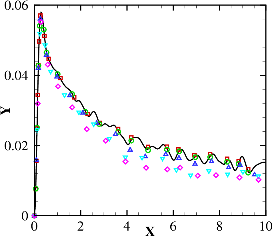
The results obtained with ATI and BW discretization in all space directions are shown in Figs. 3 and 4, respectively, at various Courant numbers. Stable results are obtained for for ATI, and for BW. Loss of stability at larger time steps is due to flux linearization and/or factorization errors, which prevent unconditional stability in practical computations [12]. The time behavior of turbulence kinetic energy (panel (a)) is well predicted at all Courant numbers up to the stability limit, whereas pressure fluctuations (panel (b)) are overdamped starting at , in both ATI and BW. The different behavior is caused by the fact that pressure receives contributions of both hydrodynamic and acoustic nature. As seen in the previous Section, acoustic waves undergo significant damping at high Courant number. This is even clearer in the velocity and pressure spectra, shown in panels (c) and (d), respectively. While velocity spectra are perfectly captured at all Courant numbers, pressure spectra undergo numerical damping, especially at intermediate wavenumbers, which is easily understood based on the amplification factors shown in Fig. 2. Given the similar performance of the two implicit methods for this test case, ATI is certainly preferable owing to its lower computational cost, which allows to achieve an effective speed-up over the explicit case (see table 1) of about a factor of three, whereas BW yields almost the same efficiency.
3.2 Turbulent flow in plane channel
Channel flow is the simplest prototype of wall-bounded flows, and it has been studied by many authors in the incompressible [42, 43, 1], as well as in the compressible regime [44, 45, 5]. The controlling parameters are the bulk Mach number (where is the average velocity across the channel thickness, and the sound speed at the wall temperature), and the bulk Reynolds number (where is the bulk density, the dynamic viscosity at the wall, and the channel half height). All DNS are initialized with a parabolic velocity profile with superposed small perturbations, whereas density and pressure are uniform. Periodic boundary conditions are applied in the streamwise () and spanwise () coordinate directions, and no-slip, isothermal boundary conditions are applied at the walls. A spatially uniform forcing is applied to the streamwise momentum equation, and dynamically adjusted in time to maintain constant mass flow rate [5]. Favre density-weighted decomposition is applied to separate mean values from fluctuations, namely , with ).
| Case | CPU | ||||||||||||
|---|---|---|---|---|---|---|---|---|---|---|---|---|---|
| CH01-EXPL | 0.1 | 0.1 | 5790 | 180 | 0.60 | 8.80 | 3.90 | 0.053 | 0.0077 | 0.026 | 1.3 | 0.0077 | 1 |
| CH01-ATI-XYZ | 0.1 | 0.1 | 5790 | 180 | 0.60 | 8.80 | 3.90 | 0.053 | 0.0077 | 0.026 | 1.3 | 0.077 | 0.15 |
| CH01-BW-XYZ | 0.1 | 0.1 | 5790 | 180 | 0.60 | 8.80 | 3.90 | 0.053 | 0.0077 | 0.026 | 1.3 | 0.077 | 0.82 |
| CH15a-EXPL | 1.5 | 1.28 | 6000 | 220 | 0.70 | 10.8 | 4.80 | 0.32 | 0.11 | 0.27 | 1.2 | 0.099 | 1 |
| CH15a-ATI-Y | 1.5 | 1.28 | 6000 | 220 | 0.70 | 10.8 | 4.80 | 0.32 | 0.11 | 0.27 | 1.2 | 0.24 | 0.48 |
| CH15a-BW-Y | 1.5 | 1.28 | 6000 | 220 | 0.70 | 10.8 | 4.80 | 0.32 | 0.11 | 0.27 | 1.2 | 0.24 | 0.70 |
| CH15b-EXPL | 1.5 | 1.28 | 6000 | 220 | 0.15 | 10.8 | 4.08 | 0.32 | 0.11 | 0.27 | 0.062 | 0.021 | 1 |
| CH15b-AVTI-Y | 1.5 | 1.28 | 6000 | 220 | 0.15 | 10.8 | 4.80 | 0.32 | 0.11 | 0.27 | 0.062 | 0.21 | 0.13 |
| CH15b-BWV-Y | 1.5 | 1.28 | 6000 | 220 | 0.15 | 10.8 | 4.80 | 0.32 | 0.11 | 0.27 | 0.062 | 0.21 | 0.19 |
The main flow parameters are listed in Tab. 2. Three flow cases have been considered, one at (denoted as CH01), and two at (denoted as CH15a-b), the latter two only differing in the distance of the first grid point from the wall. Reference DNS have been carried out with fully explicit time discretization, at , which are used as a basis of comparison for the ATI and BW algorithms. In order to understand the effectiveness of the (semi-)implicit algorithms, in Tab. 2 we report the time step restrictions associated with the three coordinate directions, as estimated from Eqns. (1),(3), as well as the actual time step used in the DNS, all in wall units. As expected, in all flow cases the time step limitation in the wall-normal direction is the most restrictive. Although larger time steps are allowed on grounds of sole numerical stability, all DNS have been carried out at the maximum time step for which accurate results are obtained, which corresponds to for the fully explicit simulations. For ease of reference, the maximum time steps associated with accuracy and stability restrictions are also reported in Fig. 1(a) with circle and square symbols, respectively.
As a first test, we consider flow at low subsonic Mach number (CH01), for which the explicit time advancement step is very small, hence we apply implicit treatment is all coordinate directions (XYZ). We find that, although the wall-normal time step restrictions can be removed, the allowed time step for accurate calculations cannot substantially larger than for the streamwise convective restriction (see Fig. 1(a)). This is probably due to inherent mesh anisotropy in DNS of wall-bounded flows. In fact, mesh spacing is over-resolved in the wall-normal direction, hence the relevant values of the reduced wavenumber are small, which allows to operate at high values of with little error, recalling (see Fig. 2) that the dissipation error grows with both and . On the other hand, the typical wall-parallel mesh spacings used in DNS are barely sufficient to resolve the smallest scales of turbulence, hence the typical reduced wavenumbers are higher, and time accuracy is a factor in that case. We find that both ATI and BW are capable of boosting the time step by about a factor of ten, with efficiency gain of for ATI, and results almost indistinguishable from the fully explicit case (see below). Still, the time step is far from that allowed by incompressible solvers (again, see Fig. 1(a)). This issue will be further recalled in the concluding discussion.
To show effectiveness in removing the wall-normal acoustic time limitation is supersonic flow calculations, in flow case CH15a the first grid point is placed sufficiently far from the wall that the viscous limitation is ineffective. Hence, the implicit algorithms are applied only in the wall-normal direction (Y), and viscous terms are handled explicitly. The ATI and BW algorithms are both found to effectively suppress the wall-normal acoustic time step limitation, and achieve the same maximum time step for accurate flow resolution, corresponding to about . Hence, accounting for the cost figures given in table 1, we find a speed-up of about a factor of two for the ATI algorithm, and gain with BW.
To prove effectiveness of the implicit treatment of the viscous terms proposed in Section (2.2), in flow case CH15b the first grid point is placed closer to the wall, in such a way that the viscous time limitation also becomes relevant, after the acoustic one. Both wall-normal time step restrictions are suppressed through use of the AVTI and BWV algorithms, hence the achieved time step is similar to flow case CH15a. Both algorithms here achieve , at a cost which is a small fraction of the fully explicit algorithm.
For the sake of comparison, in Figs. 5-7 we show the main statistics for the flow cases listed in Table 2. As anticipated, excellent agreement is observed between implicit algorithms and the reference explicit solution, including pressure and temperature fluctuations, which is especially satisfactory.
(a)
 (b)
(b)

(c)
 (d)
(d)

(a)
 (b)
(b)

(c)
 (d)
(d)

(a)
 (b)
(b)

(c)
 (d)
(d)

3.3 Turbulent flow in square duct
| Case | CPU | ||||||||||||
|---|---|---|---|---|---|---|---|---|---|---|---|---|---|
| DU02-EXPL | 0.2 | 0.2 | 4410 | 150 | 0.66 | 8.40 | 0.66-3.20 | 0.094 | 0.019 | 0.019 | 1.69 | 0.018 | 1 |
| DU02-ATI-XYZ | 0.2 | 0.2 | 4410 | 150 | 0.66 | 8.40 | 0.66-3.20 | 0.094 | 0.019 | 0.019 | 1.69 | 0.18 | 0.15 |
As a further step in complexity we consider the flow inside a straight duct with square cross-section. This flow has been the subject of several DNS studies in the incompressible regime [46, 47, 48], all limited to low Reynolds number. One of the main difficulties that arise when dealing with square duct flows is the long averaging time necessary to attain convergence of even the basic mean flow statistics, caused by the extremely long typical time scales of secondary corner eddies. In fact, Pinelli et al. [48] reported that an averaging time of about was needed to have symmetric statistics in the four quadrants of the cross section. Hence, it is clear that efficient numerical methods are needed to study turbulent compressible flow in ducts. Numerical simulations have been here carried out (see Table 3 for the main flow parameters) at the same Reynolds number as Pinelli et al. [48], and sufficiently low Mach number () that direct comparison with incompressible data is possible. The duct length (where is the length of each side of the duct), and the time window for collecting the flow statistics is the same used by Pinelli et al. [48]. As in plane channel flow, a spatially uniform forcing is applied to the momentum equation to maintain a time constant mass flow rate. Note that, unlike in channel flow, the mesh is also non-uniformly spaced in the direction, hence a range of mesh spacings is reported in Table 3. A reference fully explicit numerical simulation has been carried out and used as a basis of reference for the ATI algorithm, here applied to all coordinate directions. As seen in Table 3, the corresponding CFL number is about unity. As in the case of plane channel, DNS were carried out at increasing values of CFL, until deviations from the reference data were found, to determine the maximum allowed time step for accuracy. It appears that accurate results of the semi-implicit algorithm are recovered up to . Again, implicit treatment of the direction is not capable of fully suppressing the corresponding time step limitation, owing to the emergence of accuracy issues. Similar to channel flow, use of the ATI algorithm allows for about cost reduction. Figure 8 confirms that excellent matching of the flow statistics is found among DU02-ATI, DU02-EXPL and the data of Pinelli et al. [48], except for some differences in the wall-normal Reynolds stress and the pressure r.m.s., which may be due to the greater importance of acoustic waves in the presence of a fully confined flow geometry.
(a)
 (b)
(b)

(c)
 (d)
(d)

4 Conclusions
A novel semi-implicit algorithm for time-accurate solution of the compressible Navier-Stokes equations has been developed, which is capable to operate efficiently all the way from low subsonic to supersonic flow conditions. The main features of the algorithm are as follows: i) use of the entropy transport equation instead of total energy conservation; ii) Beam-Warming-like linearization of the partial convective flux associated with acoustic propagation; iii) energy-consistent discretization of the convective derivatives in the explicit part of the time-advancement operator; iv) semi-implicit treatment of viscous fluxes based on isolation of Laplacian terms; v) approximate factorization for implicit treatment of multiple space directions; vi) third-order accurate Runge-Kutta time integration, according to the algorithm proposed by Nikitin [34]. The main advantage of the algorithm is that, unlike the classical Beam-Warming scheme, it avoids the computationally expensive inversion of block-banded matrices, but rather of standard banded matrices (tridiagonal matrices in the case of second-order accurate space discretization). Specifically, a single banded matrix inversion is needed for implicit treatment of the convective terms, whereas five matrix inversions are needed if viscous terms are also handled implicitly. The cost overhead with respect to standard explicit algorithms (see Table 1) is quite modest, ranging from to , for each space direction to be handled implicitly. Modification of existing compressible flow solvers to incorporate the present method is straightforward, as the explicit part of the algorithm is unchanged.
The method nominally allows unconditional stability for low-Mach-number flows. However, flux linearization and approximate factorization reduce the stability margins, and CFL number of the order of 5-10 are achieved in practical computations, which is probably less than achievable with iterative methods. However, compared to compressible flow algorithms based on pre-conditioning, the present method avoids use of inner time iterations, whose computational cost is difficult to estimate a-priori. The other possible shortcoming of the method is the use of the entropy equation, which is instrumental to achieve (approximate) separation of hydrodynamic from acoustic effects. While use of the entropy equation yields improved numerical stability, it also makes proper capturing of shock waves difficult, as the equations are not in conservation form. We have found that this issue can be fixed by locally reverting to a total energy formulation for the explicit time increment in the presence of shocks, as identified through a shock sensor [38]. The resulting time increments are then converted to the entropy increments, prior to application of the implicit operator.
Although the algorithm herein developed has in principle much wider range of applications, the main focus of this paper was on DNS of compressible wall-bounded flows, which is notoriously plagued by severe time step restrictions inherited from the wall-normal acoustic and viscous stability conditions. We have found that the wall-normal acoustic time limitation can be effectively removed through semi-implicit treatment. The same conclusion also applies to the viscous time step restriction, although the most efficient way to remove it is placing the first grid point sufficiently away from the wall , and using suitable staggering [5], with no effect of accuracy. The wall-parallel stability restrictions can also be suppressed through semi-implicit treatment. However, accuracy considerations lead to the practical rule (see Fig. 1) that the time step cannot be much larger than the one stemming from the streamwise time limitation. Hence, we suggest that in low-subsonic flow both the wall-normal and the spanwise convective terms are handled implicitly, whereas the streamwise terms can be evaluated explicitly. The resulting saving of computer time can then be of the order of with respect to a fully explicit solver. In high subsonic or supersonic flow, implicit treatment of the wall-normal convective derivatives is sufficient, with typical savings of to order of , in line with theoretical estimates.
We foresee that the present technique can be fruitfully extended to numerical simulation
of wall-bounded turbulent flows with time-accurate models, such as LES or DES [49].
In that case, given the higher aspect ratio of near-wall cells, higher gains are expected.
Advantages with respect to classical algorithms based on Beam-Warming linearization are also
expected for steady RANS applications. Indeed, although the present algorithm is in principle
only capable of suppressing the acoustic time step limitation, it is found to be at least as
stable as Beam-Warming in practical computations.
Acknowledgements
We acknowledge that most of the results reported in this paper have been achieved using the PRACE Research Infrastructure resource FERMI based at CINECA, Casalecchio di Reno, Italy.
References
- [1] M. Lee, R. Moser, Direct simulation of turbulent channel flow layer up to Re, J. Fluid Mech. 774 (2015) 395–415.
- [2] S. Lele, Compressibility effects on turbulence, Annu. Rev. Fluid Mech. 26 (1994) 211–254.
- [3] T. Poinsot, A. Trouve, D. Veynante, S. Candel, E. Esposito, Vortex-driven acoustically coupled combustion instabilities, J. Fluid Mech. 177 (1987) 265–292.
- [4] T. Colonius, S. K. Lele, Computational aeroacoustics: progress on nonlinear problems of sound generation, Progr. Aero. Sci. 40 (2004) 345–416.
- [5] D. Modesti, S. Pirozzoli, Reynolds and Mach number effects in compressible turbulent channel flow, Int. J. Heat Fluid Flow 59 (2016) 33–49.
- [6] R. Beam, R. Warming, An implicit finite-difference algorithm for hyperbolic systems in conservation-law form, J. Comput. Phys. 22 (1976) 87–110.
- [7] R. Beam, R. Warming, An implicit factored scheme for the compressible Navier-Stokes equations, AIAA J. 16 (1978) 393–402.
- [8] J. Douglas, On the Numerical Integration of by Implicit Methods, J. Soc. Ind. Appl. Math 3 (1955) 42–65.
- [9] E. Isaacson, H. Keller, Analysis of numerical methods, Courier Corporation, 1994.
- [10] M. Batista, A cyclic block-tridiagonal solver, Adv. Eng. Softw. 37 (2006) 69–74.
- [11] T. Pulliam, D. Chaussee, A diagonal form of an implicit approximate-factorization algorithm, J. Comput. Phys. 39 (1981) 347–363.
- [12] C. Hirsch, Numerical computation of internal and external flows: The fundamentals of computational fluid dynamics, Butterworth-Heinemann, 2007.
- [13] T. Pulliam, Solution methods in computational fluid dynamics (1986).
- [14] P. Buning, D. Jespersen, H. Thomas, W. Chan, J. Slotnick, S. Krist, K. Renze, OVERFLOW user’s manual, NASA Langley Research Center.
- [15] M. Martín, G. Candler, A parallel implicit method for the direct numerical simulation of wall-bounded compressible turbulence, J. Comput. Phys. 215 (2006) 153–171.
- [16] E. Turkel, Review of preconditioning methods for fluid dynamics, Appl. Numer. Math. 12 (1993) 257–284.
- [17] E. Turkel, Preconditioning techniques in computational fluid dynamics, Annu. Rev. Fluid Mech. 31 (1999) 385–416.
- [18] S. Venkateswaran, C. Merkle, Dual time stepping and preconditioning for unsteady computations, AIAA Paper 1995-0078 (1995).
- [19] S. Pandya, S. Venkateswaran, T. Pulliam, Implementation of preconditioned dual-time procedures in OVERFLOW, AIAA paper 2003-0072 (2003).
- [20] P. D. Palma, M. D. Tullio, G. Pascazio, M. Napolitano, An immersed-boundary method for compressible viscous flows, Comput. Fluids 35 (2006) 693–702.
- [21] V. Casulli, D. Greenspan, Pressure method for the numerical solution of transient, compressible fluid flows, Int. J. Num. Meth. Fluids 4 (1984) 1001–1012.
- [22] C. Pierce, Progress-variable approach for large-eddy simulation of turbulent combustion, Ph.D. thesis, Citeseer (2001).
- [23] C. Wall, C. Pierce, P. Moin, A semi-implicit method for resolution of acoustic waves in low Mach number flows, J. Comput. Phys. 181 (2002) 545–563.
- [24] J. Kim, P. Moin, Application of a fractional-step method to incompressible Navier-Stokes equations, J. Comput. Phys. 59 (1985) 308–323.
- [25] V. Moureau, C. Bérat, H. Pitsch, An efficient semi-implicit compressible solver for large-eddy simulations, J. Comput. Phys. 226 (2007) 1256–1270.
- [26] P. Spalart, R. Moser, M. Rogers, Spectral methods for the Navier-Stokes equations with one infinite and two periodic directions, J. Comput. Phys. 96 (1991) 297–324.
- [27] J. Sesterhenn, A characteristic-type formulation of the navier-stokes equations for high order upwind schemes, Comput. Fluids 30 (2000) 37–67.
- [28] A. Honein, P. Moin, Higher entropy conservation and numerical stability of compressible turbulence simulations, J. Comput. Phys. 201 (2004) 531–545.
- [29] M. Salas, A. Iollo, Entropy jump across an inviscid shock wave, Theor. Comp. Fluid Dyn. 8 (1996) 365–375.
- [30] L. Kovásznay, Turbulence in supersonic flow, J. Aero. Sci. 20 (1953) 657–674.
- [31] J. Steger, Coefficient matrices for implicit finite difference solution of the inviscid fluid conservation law equations, Comput. Meth. Appl. Mech. Eng. 13 (1978) 175–188.
- [32] T. Barth, J. Steger, A fast efficient implicit scheme for the gasdynamics equations using a matrix reduction technique, AIAA paper 1985-0085 (1985).
- [33] P. Orlandi, Fluid flow phenomena: a numerical toolkit, Kluwer, 2000.
- [34] N. Nikitin, Third-order-accurate semi-implicit Runge-Kutta scheme for incompressible Navier-Stokes equations, Int. J. Num. Meth. Fluids 51 (2006) 221–233.
- [35] R. Vichnevetsky, J. B. Bowles, Fourier analysis of numerical approximations of hyperbolic equations, SIAM, Philadelphia, 1982.
- [36] S. Pirozzoli, Generalized conservative approximations of split convective derivative operators, J. Comput. Phys. 229 (2010) 7180–7190.
- [37] C. Kennedy, A. Gruber, Reduced aliasing formulations of the convective terms within the Navier-Stokes equations for a compressible fluid, J. Comput. Phys. 227 (2008) 1676–1700.
- [38] S. Pirozzoli, Numerical methods for high-speed flows, Annu. Rev. Fluid Mech. 43 (2011) 163–194.
- [39] S. K. Lele, Compact finite difference schemes with spectral-like resolution, J. Comput. Phys. 103 (1992) 16.
- [40] M. Shoeybi, M. Svärd, F. Ham, P. Moin, An adaptive implicit-explicit scheme for the DNS and LES of compressible flows on unstructured grids, J. Comput. Phys. 229 (17) (2010) 5944–5965.
- [41] G. Blaisdell, N. Mansour, W. Reynolds, Numerical simulation of compressible homogeneous turbulence, Report TF-50, Thermosciences Division,Dep. Mech. Eng., Stanford University (1991).
- [42] J. Kim, P. Moin, R. Moser, Turbulence statistics in fully developed channel flow at low Reynolds number, J. Fluid Mech. 177 (1987) 133–166.
- [43] M. Bernardini, S. Pirozzoli, P. Orlandi, Velocity statistics in turbulent channel flow up to Re, J. Fluid Mech. 742 (2014) 171–191.
- [44] G. Coleman, J. Kim, R. Moser, A numerical study of turbulent supersonic isothermal-wall channel flow, J. Fluid Mech. 305 (1995) 159–183.
- [45] R. Lechner, J. Sesterhenn, R. Friedrich, Turbulent supersonic channel flow, J. Turbul. 2 (2001) 1–25.
- [46] S. Gavrilakis, Numerical simulation of low-Reynolds-number turbulent flow through a straight square duct, J. Fluid Mech. 244 (1992) 101–129.
- [47] A. Huser, S. Biringen, Direct numerical simulation of turbulent flow in a square duct, J. Fluid Mech. 257 (1993) 65–95.
- [48] A. Pinelli, M. Uhlmann, A. Sekimoto, G. Kawahara, Reynolds number dependence of mean flow structure in square duct turbulence, J. Fluid Mech. 644 (2010) 107–122.
- [49] P. Spalart, Strategies for turbulence modelling and simulations, Int. J. Heat Fluid Flow 21 (2000) 252–263.