Effect of a Locally Repulsive Interaction on s–wave Superconductors

Theoretical foundations of superconductivity go back to the celebrated BCS theory – appeared in the late fifties (1957) – which explains conventional type I superconductors. This theory is based on the so–called (reduced) BCS Hamiltonian

$$\mathrm{H}_{\Lambda}^{BCS}:=\sum\limits_{k\in\Lambda^{\ast}}\left(\varepsilon_{k}-\mu\right)\left(\tilde{a}_{k,\uparrow}^{\ast}\tilde{a}_{k,\uparrow}+\tilde{a}_{k,\downarrow}^{\ast}\tilde{a}_{k,\downarrow}\right)+\frac{1}{|\Lambda|}\sum_{k,k^{\prime}\in\Lambda^{\ast}}\gamma_{k,k^{\prime}}\tilde{a}_{k,\uparrow}^{\ast}\tilde{a}_{-k,\downarrow}^{\ast}\tilde{a}_{k^{\prime},\downarrow}\tilde{a}_{-k^{\prime},\uparrow}$$

(1.1)

defined in a cubic box $\Lambda\subset\mathbb{R}^{3}$ of volume $|\Lambda|$. Here $\Lambda^{\ast}$ is the dual group of $\Lambda$ seen as a torus (periodic boundary condition) and the operator $\tilde{a}_{k,s}^{\ast}$ resp. $\tilde{a}_{k,s}$ creates resp. annihilates a fermion with spin $s\in\{\uparrow,\downarrow\}$ and momentum $k\in\Lambda^{\ast}$. The function $\varepsilon_{k}$ represents the kinetic energy, the real number $\mu$ is the chemical potential and $\gamma_{k,k^{\prime}}$ is the BCS coupling function. The choice $\gamma_{k,k^{\prime}}=-\gamma<0$ is often used in the Physics literature and the case $\varepsilon_{k}=0$ is known as the strong coupling limit of the BCS model.

The lattice approximation of the BCS Hamiltonian amounts to replace the box $\Lambda\subset\mathbb{R}^{3}$ by $\Lambda\subset\mathbb{Z}^{3}$ (or more generally by $\Lambda\subset\mathbb{Z}^{d\geq 1}$) and the strong coupling limit of the reduced BCS model is in this case known as the strong coupling (with $\gamma_{k,k^{\prime}}=-\gamma$) BCS model²² 2 See also (1.2) with $\lambda=0$ and $h=0.$. The assumptions $\epsilon_{k}=0$ and $\gamma_{k,k^{\prime}}=-\gamma$ are of interest, because in this case the BCS Hamiltonian can be explicitly diagonalised. The exact solution of the strong coupling BCS model is well–known since the sixties [6, 7]. This model is in a sense unrealistic: among other things, its representation of the kinetic energy of electrons is rather poor. Nevertheless it became popular because it displays most of basic properties of real conventional type I superconductors. See, e.g., Chapter VII, Section 4 in [8]. Even though the analysis of the thermodynamics of the BCS Hamiltonian was rigorously performed in the eighties [9, 10] (see also the innovating work of Bernadskii and Minlos in 1972 [11]), generalizations of the strong coupling approximation of the BCS model are still subject of research. For instance, strong coupling–BCS–type models with superconducting phases at arbitrarily high temperatures are treated in [12].

In fact, a general theory of superconductivity is still a subject of debate, especially for high–$T_{c}$ superconductors. An important phenomenon ignored in the BCS theory is the Coulomb interaction between electrons or holes, which can imply strong correlations, for instance in high–$T_{c}$ superconductors. To study these correlations, most of theoretical methods, inspired by Beliaev [5], use perturbation theory or renormalization group derived from the diagram approach of Quantum Field Theory. However, even if these approaches have been successful in explaining many physical properties of superconductors [3, 4], only few rigorous results exist on superconductivity.

For instance, the effect of the Coulomb interaction on superconductivity is not rigorously known. This problem was of course adressed in theoretical Physics right after the emergence of the Fröhlich model and the BCS theory, see, e.g., [13]. In particular, the authors explain in [13, Chapter VI], by means of diagrammatic pertubation theory, that the effect of the Coulomb interaction on the Fröhlich model should be to lower the critical temperature of the superconducting phase by lowering the electron density. We rigorously show that this phenomenology is only true – for our model – in a specific region of parameters.

Indeed, the aim of the present paper is to understand the possible thermodynamic impact of the Coulomb repulsion in the strong coupling approximation. More precisely, we study the thermodynamic properties of the strong coupling BCS--Hubbard model defined in the box³³ 3 Without loss of generality we choose $N$ such that $L:=(N^{1/d}-1)/2\in\mathbb{N}$. $\Lambda_{N}:=\{\mathbb{Z}\cap[-L,L]\}^{d\geq 1}$ of volume $|\Lambda_{N}|=N\geq 2$ by the Hamiltonian

	$\displaystyle\mathrm{H}_{N}:=$		$\displaystyle-\mu\sum\limits_{x\in\Lambda_{N}}\left(n_{x,\uparrow}+n_{x,\downarrow}\right)-h\sum_{x\in\Lambda_{N}}\left(n_{x,\uparrow}-n_{x,\downarrow}\right)+2\lambda\sum_{x\in\Lambda_{N}}n_{x,\uparrow}n_{x,\downarrow}$		(1.2)
			$\displaystyle-\frac{\gamma}{N}\sum_{x,y\in\Lambda_{N}}a_{x,\uparrow}^{\ast}a_{x,\downarrow}^{\ast}a_{y,\downarrow}a_{y,\uparrow}$

for real parameters $\mu$, $h$, $\lambda$, and $\gamma\geq 0$. The operator $a_{x,s}^{\ast}$ resp. $a_{x,s}$ creates resp. annihilates a fermion with spin $s\in\{\uparrow,\downarrow\}$ at lattice position $x\in\mathbb{Z}^{d}$ whereas $n_{x,s}:=a_{x,s}^{\ast}a_{x,s}$ is the particle number operator at position $x$ and spin $s$. The first term of the right hand side (r.h.s.) of (1.2) represents the strong coupling limit of the kinetic energy, with $\mu$ being the chemical potential of the system. Note that this “strong coupling limit” – explained above for the BCS Hamiltonian – is also called “atomic limit” in the context of the Hubbard model, see, e.g., [14, 15]. The second term in the r.h.s. of (1.2) corresponds to the interaction between spins and the magnetic field $h$. The one–site interaction with coupling constant $\lambda$ represents the (screened) Coulomb repulsion as in the celebrated Hubbard model. So, the parameter $\lambda$ should be taken as a positive number but our results are also valid for any real $\lambda$. The last term is the BCS interaction written in the $x$–space since

$$\frac{\gamma}{N}\sum_{x,y\in\Lambda_{N}}a_{x,\uparrow}^{\ast}a_{x,\downarrow}^{\ast}a_{y,\downarrow}a_{y,\uparrow}=\frac{\gamma}{N}\sum_{k,q\in\Lambda_{N}^{\ast}}\tilde{a}_{k,\uparrow}^{\ast}\tilde{a}_{-k,\downarrow}^{\ast}\tilde{a}_{q,\downarrow}\tilde{a}_{-q,\uparrow},$$

(1.3)

with $\Lambda_{N}^{\ast}$ being the reciprocal lattice of quasi–momenta and where $\tilde{a}_{q,s}$ is the corresponding annihilation operator for $s\in\{\uparrow,\downarrow\}$. Observe that the thermodynamics of the model for $\gamma=0$ can easily be computed. Therefore we restrict the analysis to the case $\gamma>0$. Note also that the homogeneous BCS interaction (1.3) can imply a superconducting phase and the mediator implying this effective interaction does not matter here, i.e., it could be due to phonons, as in conventional type I superconductors, or anything else.

We show that the one–site repulsion suppresses superconductivity for large $\lambda\geq 0$. In particular, the repulsive term in (1.2) cannot imply any superconducting state if $\gamma=0.$ However, the first elementary but nonetheless important property of this model is that the presence of an electron repulsion is not incompatible with superconductivity if $|\lambda-\mu|$ and $(\lambda+|h|)$ are not too big as compared to the coupling constant $\gamma$ of the BCS interaction. In this case, the superconducting phase appears at low temperatures as either a first order or a second order phase transition. More surprisingly, the one–site repulsion can even favor superconductivity at fixed chemical potential $\mu$ by increasing the critical temperature and/or the Cooper pair condensate density. This contradicts the naive guess that any one–site repulsion between electron pairs should at least reduce the formation of Cooper pairs. It is however important to mention that the physical behavior described by the model depends on which parameter, $\mu$ or $\rho,$ is fixed. (It does not mean that the canonical and grand–canonical ensembles are not equivalent for this model). Indeed, we also analyze the thermodynamic properties at fixed electron density $\rho$ per site in the grand–canonical ensemble, as it is done for the perfect Bose gas in the proof of Bose-Einstein condensation. The analysis of the thermodynamics of the strong coupling BCS–Hubbard model is performed in details. In particular, we prove that the Meißner effect is rather generic but also that the coexistence of superconducting and ferromagnetic phases is possible (as in the Vonsovkii–Zener model [16, 17]), for instance at large $\lambda>0$ and densities near half–filling. The later situation is related to a superconductor–Mott insulator phase transition. This transition gives furthermore a rigorous explanation of the need of doping insulators to obtain superconductors. Indeed, at large enough coupling constant $\lambda$, the superconductor–Mott insulator phase transition corresponds to the breakdown of superconductivity together with the appearance of a gap in the chemical potential as soon as the electron density per site becomes an integer, i.e., $0$, $1$ or $2$. If the system has an electron density per site equal to $1$ without being superconductor, then any non–zero magnetic field $h\neq 0$ implies a ferromagnetic phase.

Note that the present setting is still too simplified with respect to (w.r.t.) real superconductors. For instance, the anti–ferromagnetic phase or the presence of vortices, which can appear in (type II) high–$T_{c}$ superconductors [3, 4], are not modeled. However, the BCS–Hubbard Hamiltonian (1.2) may be a good model for certain kinds of superconductors or ultra-cold Fermi gases in optical lattices, where the strong coupling approximation is experimentally justified. Actually, even if the strong coupling assumption is a severe simplification, it may be used in order to analyze the thermodynamic impact of the Coulomb repulsion, as all parameters of the model have a phenomenological interpretation and can be directly related to experiments. See discussions in Section 5. Moreover, the range of parameters in which we are interested turns out to be related to a first order phase transition. This kind of phase transitions are known to be stable under small perturbations of the Hamiltonian. In particular, by including a small kinetic part it can be shown by high–low temperature expansions that the model

$$\mathrm{H}_{N,\varepsilon}:=\mathrm{H}_{N}+\sum\limits_{x,y\in\Lambda_{N}}\varepsilon(x-y)\left(a_{y,\downarrow}^{\ast}a_{x,\downarrow}+a_{y,\uparrow}^{\ast}a_{x,\uparrow}\right)$$

has essentially the same correlation functions as $\mathrm{H}_{N}$, up to corrections of order $||\varepsilon||_{1}$ ($\ell^{1}$–norm of $\varepsilon$). This analysis will be the subject of a separated paper. For any $\varepsilon\neq 0$ notice that the model $\mathrm{H}_{N,\varepsilon}$ is not anymore permutation invariant but only translation invariant. Such translation invariant models are studied in a systematic way in [18]. Their detailed analysis is however, generally much more difficult to perform. Considering first models having more symmetries – as for instance, permutation invariance – is in this case technically easier.

Coming back to the strong coupling BCS–Hubbard model $\mathrm{H}_{N}$, it turns out that the thermodynamic limit of its (grand--canonical) pressure⁴⁴ 4 Our notation for the “$\mathrm{Trace"}$ does not include the Hilbert space where it is evaluated but it should be deduced from operators involved in each statement.

$$\mathrm{p}_{N}\left(\beta,\mu,\lambda,\gamma,h\right):=\frac{1}{\beta N}\ln\mathrm{Trace}\left(e^{-\beta\mathrm{H}_{N}}\right)$$

(1.4)

exists at any fixed inverse temperature $\beta>0$. It corresponds to a variational problem which has minimizers⁵⁵ 5 Because $\omega\mapsto\mathfrak{F}(\omega)$ is lower semicontinuous and $E_{\mathcal{U}}^{S,+}$ is compact with respect to the weak^∗–topology. in the set $E_{\mathcal{U}}^{S,+}$ of (even⁶⁶ 6 See Remark 6.1 in Section 6.1.) permutation invariant states on the CAR $C^{\ast}$–algebra $\mathcal{U}$ generated by annihilation and creation operators:

$$\mathrm{p}\left(\beta,\mu,\lambda,\gamma,h\right):=\lim\limits_{N\rightarrow\infty}\left\{\mathrm{p}_{N}\left(\beta,\mu,\lambda,\gamma,h\right)\right\}=-\inf\limits_{\omega\in E_{\mathcal{U}}^{S,+}}\mathfrak{F}\left(\omega\right).$$

(1.5)

Here the map

$$\omega\mapsto\mathfrak{F}(\omega):=\mathfrak{e}(\omega)-\beta^{-1}\tilde{S}(\omega)$$

is the affine (lower weak^∗–semicontinuous) free–energy density functional defined on $E_{\mathcal{U}}^{S,+}$ from the mean energy per volume

$$\mathfrak{e}\left(\omega\right):=\lim\limits_{N\rightarrow\infty}\left\{N^{-1}\omega\left(\mathrm{H}_{N}\right)\right\}<\infty$$

and the entropy density

$$\tilde{S}\left(\omega\right):=-\lim\limits_{N\rightarrow\infty}\left\{\frac{1}{N}\mathrm{Trace}\left(D_{\omega|_{{\mathcal{U}}_{N}}}\log D_{\omega|_{{\mathcal{U}}_{N}}}\right)\right\}<\infty.$$

Note that $D_{\omega|_{{\mathcal{U}}_{N}}}$ is the density matrix associated to the state $\omega$ restricted on the local CAR $C^{\ast}$–algebra ${\mathcal{U}}_{N}\simeq B\left(\bigwedge\mathbb{C}^{\Lambda_{N}\times\{\uparrow,\downarrow\}}\right)$ (isomorphism). Such a derivation of the pressure as a minimization problem over states on a $C^{\ast}$–algebras are also performed for various quantum spin systems, see, e.g., [19, 20, 21, 22, 23].

The minimum of the variational problem (1.5) is attained for any weak^∗–limit point of local Gibbs states

$$\omega_{N}\left(\cdot\right):=\frac{\mathrm{Trace}\left(\mathrm{\ }\cdot\mathrm{\ }e^{-\beta\mathrm{H}_{N}}\right)}{\mathrm{Trace}\left(e^{-\beta\mathrm{H}_{N}}\right)}$$

(1.6)

associated with $\mathrm{H}_{N}$. Similarly to what is done for general translation invariant models (see [24, 25]), the set of equilibrium states of the strong coupling BCS–Hubbard model is naturally defined to be the set $\mathit{\Omega}_{\beta}=\mathit{\Omega}_{\beta}(\mu,\lambda,\gamma,h)$ of minimizers of (1.5). Note that $\mathit{\Omega}_{\beta}$ is a non empty convex subset⁷⁷ 7 The map $\omega\mapsto\mathfrak{F}(\omega)$ on the convex set $E_{\mathcal{U}}^{S,+}$ is affine and lower semicontinuous, thus $\mathit{\Omega}_{\beta}$ is a non empty face of $E_{\mathcal{U}}^{S,+}$. of $E_{\mathcal{U}}^{S,+}$ and the extremal decomposition in $\mathit{\Omega}_{\beta}$ coincides with the one in $E_{\mathcal{U}}^{S,+}$, i.e., $\mathit{\Omega}_{\beta}$ is a face⁸⁸ 8 A face $\mathrm{F}$ of a compact convex set $\mathrm{K}$ is subset of $\mathrm{K}$ with the property that if $\omega=\Sigma_{n=1}^{m}\lambda_{n}\omega_{n}\in\mathrm{F}$ with $\Sigma_{n=1}^{m}\lambda_{n}=1$ and $\{\omega_{n}\}_{n=1}^{m}\subset\mathrm{K}$, then $\{\omega_{n}\}_{n=1}^{m}\subset\mathrm{F}$. in $E_{\mathcal{U}}^{S,+}$. So, pure equilibrium states are extremal states of $\mathit{\Omega}_{\beta}.$ Meanwhile, any weak^∗ limit point as $n\rightarrow\infty$ of an equilibrium state sequence $\{\omega^{(n)}\}_{n\in\mathbb{N}}$ with diverging inverse temperature $\beta_{n}\rightarrow\infty$ is – per definition – a ground state $\omega\in E_{\mathcal{U}}^{S,+}$.

Here we have left the Fock space representation of the model to go to a representation–free formulation of thermodynamic phases. This means that $\mathrm{H}_{N}$ is not anymore seen as a Hamiltonian acting on the Fock space but as a (self–adjoint) element of the CAR $C^{\ast}$–algebra $\mathcal{U}$ with thermodynamic phases describes by states on $\mathcal{U}$. Doing so we take advantage of the non–uniqueness of the representation of the CAR $C^{\ast}$–algebra $\mathcal{U}$. This property is indeed necessary to get non–unique equilibrium and ground states which imply phase transitions. This fact was first observed by R. Haag in 1962 [26], who established that the non--uniqueness of the ground state of the BCS model in infinite volume is related to the existence of several inequivalent⁹⁹ 9 This means that there is no isomorphism between $\mathfrak{h}_{j_{1}}$ and $\mathfrak{h}_{j_{2}}$ whenever $\mathfrak{h}_{j_{1}}$ and $\mathfrak{h}_{j_{2}}$ are the Hilbert spaces corresponding to two different irreducible representations. irreducible representations¹⁰¹⁰ 10 This means that the Hamiltonian can be seen as an operator acting on several Hilbert spaces $\{\mathfrak{h}_{j}\}_{j\in J}$ with no (non-trivial) invariant subspace. of the Hamiltonian, see also [6, 27].

Equilibrium states define tangents to the convex map

$$\left(\beta,\mu,\lambda,\gamma,h\right)\mapsto\mathrm{p}\left(\beta,\mu,\lambda,\gamma,h\right).$$

The analysis of the set of tangents of this map gives hence information about the expectations of many important observables w.r.t. equilibrium states. The main technical point in the present work is therefore to find an explicit representation of the pressure by using the permutation invariance of the model in a crucial way. Indeed, we adapt to our case of fermions on a lattice the methods of [19] used to find the pressure of spin systems of mean–field type. Then, it is proven that it suffices to minimize the variational problem (1.5) w.r.t. the set $\mathcal{E}_{\mathcal{U}}^{S,+}$ of extremal states in ${E}_{\mathcal{U}}^{S,+}$. By adapting the proof of Størmer’s theorem [1] to even states on the CAR algebra, we show next that extremal, permutation invariant and even states are product states

$$\omega_{\zeta}:=\bigotimes\limits_{x\in\mathbb{Z}^{d}}\zeta_{x}$$

obtained by “copying” some one–site even state $\zeta$ to all other sites. This result is a non–commutative version of the celebrated de Finetti Theorem from (classical) probability theory [28]. Using this, the variational problem (1.5) can be drastically simplified to a minimization problem on a finite dimensional manifold. At the end, it yields to another explicit, rather simple, variational problem on $\mathbb{R}_{0}^{+}$, which can be rigorously analyzed by analytic or numerical methods to obtain the complete thermodynamic behavior of the model.

Observe however, that all correlation functions cannot be drawn from an explicit formula for the pressure by taking derivatives combined with Griffiths arguments [29, 30, 31] on the convergence of derivatives of convex functions, unless the (infinite volume) pressure is shown to be differentiable w.r.t. any perturbation. Showing differentiability of the pressure as well as the explicit computation of its corresponding derivative can be a very hard task, for instance for correlation functions involving many lattice points. By contrast, the method presented in this paper gives access to all correlation functions at once. This is one basic (mathematical) message of this method, which is generalized in [18] to all translation invariant Fermi systems without requiring any quantum spin representation.

In fact, we precisely characterize the sets $\mathit{\Omega}_{\beta}$ for all $\beta\in(0,\infty]$, where $\mathit{\Omega}_{\infty}$ is the set of ground states with parameters $\mu,$ $\gamma,$ $\lambda,$ and $h$. This detailed study yields our main rigorous results on the strong coupling BCS–Hubbard model $\mathrm{H}_{N}$, which can be summarized as follows:

• •

  There is a set of parameters $\mathcal{S}$, defining the superconducting phase, with equilibrium and ground states breaking the $U(1)$–gauge symmetry and showing off–diagonal long range order (ODLRO).

• •

  Depending on the parameters, the superconducting phase transition is either a first order or a second order phase transition.

• •

  The superconducting phase $\mathcal{S}$ is characterized by the formation of Cooper pairs (shown by proving bounds for the density–density correlations) and a depleted Cooper pair condensate, the density $\mathrm{r}_{\beta}\in[0,1/4]$ of which is defined by the gap equation.

• •

  From our proof of Størmer’s theorem [1] for even states on the CAR algebra, we observe that the superconducting phase $\mathcal{S}$ corresponds to a s–wave superconductor, i.e., a superconductor with two–point correlation function, for $x,y\in\mathbb{Z}^{d}$, $s_{1},s_{2}\in\{\uparrow,\downarrow\}$ and within $\mathcal{S}$, equal to $\omega(a_{x,s_{1}}a_{y,s_{2}})=\mathrm{r}_{\beta}^{1/2}e^{i\phi}\neq 0$ if $x=y$ and $s_{1}\neq s_{2}$, and $\omega(a_{x,s_{1}}a_{y,s_{2}})=0$ else. (Here $\omega$ is any pure state of $\mathit{\Omega}_{\beta}$; $\phi\in[0,2\pi)$ is determined by $\omega$.)

• •

  We observe the Meißner effect¹¹¹¹ 11 It is mathematically defined here by the absence of magnetization in presence of superconductivity. Steady surface currents around the bulk of the superconductor are not analyzed as it is a finite volume effect. by analyzing the relation between superconductivity and magnetization.

• •

  We establish the existence of a superconductor–Mott insulator phase transition for integer electron density per site.

• •

  The coexistence of ferromagnetic and superconducting phases is shown to be feasible at (critical) points of the boundary $\partial\mathcal{S}$ of $\mathcal{S}$, by applying the decomposition theory for states [32] on the weak^∗–compact and convex set $\mathit{\Omega}_{\beta}$.

• •

  The critical temperature $\theta_{c}$ for the superconducting phase transition w.r.t. $\lambda$, $\gamma$ or $h$ is analyzed in the case of fixed chemical potential $\mu$ and also in the case of constant electron density $\rho$. It shows that $\theta_{c}$ can be an increasing function of the positive coupling constant $\lambda>0$ at fixed $\mu\in\mathbb{R}$ but not at fixed $\rho>0$.

• •

  For $\lambda\sim\gamma$ the critical temperature $\theta_{c}$ shows – as a function of the electron density $\rho$ – the typical behavior observed (only) in high–$T_{c}$ superconductors: $\theta_{c}$ is zero or very small for $\rho\sim 1$ and is much larger for $\rho$ away from $1$. Thus, our model provides a simple rigorous microscopic explanation for such experimentally well–known behavior of high–$T_{c}$ superconductors.

• •

  Together with our study of the heat capacity, all these results can be used to fix experimentally all parameters of $\mathrm{H}_{N}$.

Note that our study of equilibrium states is reminiscent of the work of Fannes, Spohn and Verbeure [33], performed however within a different framework. By opposition with our setting, their analysis [33] concerns symmetric states on an infinite tensor product of one $C^{\ast}$–algebra and their definition of equilibrium states uses the so–called correlation inequalities for KMS–states, see [29, Appendix E].

To conclude, this paper is organized as follows. In Section 2 we give the thermodynamic limit of the pressure $\mathrm{p}_{N}$ (1.4) as well as the gap equation. Then, our main results concerning the thermodynamic properties of the model are formulated in Section 3 at fixed chemical potential $\mu$ and in Section 4 at fixed electron density $\rho$ per site. Section 5 briefly explains our result on the level of equilibrium states and gives additional remarks. In order to keep the main issues and the physical implications as transparent as possible, we reduce the technical and formal aspects to a minimum in Sections 2–5. In particular, in Sections 2–4 we only stay on the level of pressure and thermodynamic limit of local Gibbs states. The generalization of the results on the level of equilibrium and ground states is postponed to Section 6.2. Indeed, the rather long Section 6 gives the detailed mathematical foundations of our phase diagrams. In particular, in Section 6.1 we introduce the $C^{\ast}$–algebraic machinery needed in our analysis and prove various technical facts to conclude in Section 6.2 with the rigorous study of equilibrium and ground states. In Section 7, we collect some useful properties on the qualitative behavior of the Cooper pair condensate density, whereas Section 8 is an appendix on Griffiths arguments [29, 30, 31].

In order to obtain the thermodynamic behavior of the strong coupling BCS–Hubbard model $\mathrm{H}_{N}$, it is essential to get first the thermodynamic limit $N\rightarrow\infty$ of its grand–canonical pressure $\mathrm{p}_{N}$ (1.4). The rigorous derivation of this limit is performed in Section 6.1. We explain here the final result with the heuristic behind it.

The first important remark is that one can guess the correct variational problem by the so-called approximating Hamiltonian method [34, 35, 36] originally proposed by Bogoliubov Jr. [37]. In our case, the correct approximation of the Hamiltonian $\mathrm{H}_{N}$ is the $c$–dependent Hamiltonian

	$\displaystyle H_{N}\left(c\right):=$		$\displaystyle-\mu\sum_{x\in\Lambda_{N}}\left(n_{x,\uparrow}+n_{x,\downarrow}\right)-h\sum_{x\in\Lambda_{N}}\left(n_{x,\uparrow}-n_{x,\downarrow}\right)+2\lambda\sum_{x\in\Lambda_{N}}n_{x,\uparrow}n_{x,\downarrow}$		(2.7)
			$\displaystyle-\frac{\gamma}{N}\sum_{x\in\Lambda_{N}}\left(\left(Nc\right)a_{x,\uparrow}^{\ast}a_{x,\downarrow}^{\ast}+\left(N\bar{c}\right)a_{x,\downarrow}a_{x,\uparrow}\right),$

with $c\in\mathbb{C}$, see also [6, 7]. The main advantage of this Hamiltonian in comparison with $\mathrm{H}_{N}$ is the fact that it is a sum of shifts of the same local operator. For an appropriate order parameter $c\in\mathbb{C}$, it leads to a good approximation of the pressure $\mathrm{p}_{N}$ as $N\rightarrow\infty$. This can be partially seen from the inequality

$$\gamma N\left|c\right|^{2}+H_{N}\left(c\right)-\mathrm{H}_{N}=\frac{\gamma}{N}\left(\sum_{x\in\Lambda_{N}}a_{x,\uparrow}^{\ast}a_{x,\downarrow}^{\ast}-N\bar{c}\right)\left(\sum_{x\in\Lambda_{N}}a_{x,\uparrow}a_{x,\downarrow}-Nc\right)\geq 0,$$

which is valid as soon as $\gamma\geq 0$. Observe that the constant term $\gamma N|c|^{2}$ is not included in the definition of $H_{N}(c)$. Hence, by using the Golden-Thompson inequality $\mathrm{Trace}(e^{A+B^{\ast}B})\leq\mathrm{Trace}(e^{A})$, the thermodynamic limit $\mathrm{p}(\beta,\mu,\lambda,\gamma,h)$ of the pressure $\mathrm{p}_{N}$ (1.4) is bounded from below by

$$\mathrm{p}\left(\beta,\mu,\lambda,\gamma,h\right)\geq\underset{c\in\mathbb{C}}{\sup}\left\{-\gamma|c|^{2}+p\left(c\right)\right\}.$$

(2.8)

The function $p\left(c\right)=p(\beta,\mu,\lambda,\gamma,h;c)$ is the pressure associated with $H_{N}(c)$ for any $N\geq 1$. It can easily be computed since $H_{N}(c)$ is a sum of local operators which commute with each other. Indeed, for any $N\geq 1,$ this pressure equals¹²¹² 12 Here $a_{0,\uparrow},$ $a_{0,\downarrow}$ and $n_{0,\uparrow},$ $n_{0,\downarrow}$ are replaced respectively by $a_{\uparrow}$, $a_{\downarrow}$ and $n_{\uparrow},$ $n_{\downarrow}.$

	$\displaystyle p\left(c\right):=$		$\displaystyle\frac{1}{\beta N}\ln\mathrm{Trace}\left(e^{-\beta H_{N}\left(c\right)}\right)=\frac{1}{\beta}\ln\mathrm{Trace}\left(e^{-\beta H_{1}\left(c\right)}\right)$		(2.9)
		$\displaystyle=$	$\displaystyle\frac{1}{\beta}\ln\mathrm{Trace}\left(e^{\beta\left\{(\mu+h)n_{\uparrow}+(\mu-h)n_{\downarrow}+\gamma(ca_{\downarrow}^{\ast}a_{\uparrow}^{\ast}+\bar{c}a_{\uparrow}a_{\downarrow})-2\lambda n_{\uparrow}n_{\downarrow}\right\}}\right).$

To be useful, the variational problem in (2.8) should also be an upper bound of $\mathrm{p}(\beta,\mu,\lambda,\gamma,h).$ By adapting the proof of Størmer’s theorem [1] to even states on the CAR algebra and by using the Petz–Raggio–Verbeure proof for spin systems [19] as a guideline, we prove this in Section 6.1. Thus, the thermodynamic limit of the pressure of the model $\mathrm{H}_{N}$ exists and can explicitly be computed by using the approximating Hamiltonian $H_{N}(c)$:

From the gauge invariance of the map $c\mapsto p(c)$ observe that any maximizer $\mathrm{c}_{\beta}\in\mathbb{C}$ of the first variational problem given in Theorem 2.1 has the form $\mathrm{r}_{\beta}^{1/2}e^{i\phi}$ with $\mathrm{r}_{\beta}\geq 0$ being solution of

$$\underset{r\geq 0}{\sup}\,f(r)=f(\mathrm{r}_{\beta})$$

(2.10)

and $\phi\in[0,2\pi)$. For any $\beta,\gamma>0$ and real numbers $\mu,\lambda,h,$ it is also clear that the order parameter $\mathrm{r}_{\beta}$ is always bounded since $f(r)$ diverges to $-\infty$ when $r\rightarrow\infty.$ Up to (special) points $(\beta,\mu,\lambda,\gamma,h)$ corresponding to a phase transition of first order, it is always unique and continuous w.r.t. each parameter (see Section 7).

For low inverse temperatures $\beta$ (high temperature regime) $\mathrm{r}_{\beta}=0$. Indeed, straightforward computations at low enough $\beta$ show that the function $f(r)$ is concave as a function of $r\geq 0$ whereas $\partial_{r}f(0)<0$, see Section 7. On the other hand, any non–zero solution $\mathrm{r}_{\beta}$ of the variational problem (2.10) has to be solution of the gap equation (or Euler–Lagrange equation)

$$\tanh\left(\beta g_{\mathrm{r}_{\beta}}\right)=\frac{2g_{\mathrm{r}_{\beta}}}{\gamma}\left(1+\frac{e^{\lambda\beta}\cosh\left(\beta h\right)}{\cosh\left(\beta g_{\mathrm{r}_{\beta}}\right)}\right).$$

(2.11)

If $g_{r}=0,$ observe that one uses in (2.11) the asymptotics $x^{-1}\tanh x\sim 1$ as $x\rightarrow 0,$ see also (7.94). Because $\tanh(x)\leq 1$ for $x\geq 0,$ we then conclude that

$$0\leq\mathrm{r}_{\beta}\leq\max\left\{0,\mathrm{r}_{\max}\right\},\mathrm{\ with\;r}_{\max}:=\frac{1}{4}-\gamma^{-2}\left(\mu-\lambda\right)^{2}.$$

(2.12)

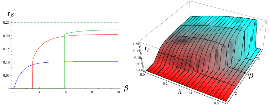
In particular, if $\gamma\leq 2|\mu-\lambda|,$ then $\mathrm{r}_{\beta}=0$ for any $\beta>0$. However, at large enough $\beta>0$ (low temperature regime) and at fixed $\lambda,h,\mu\in\mathbb{R}$, there is a unique $\gamma_{c}>2|\lambda-\mu|$ such that $\mathrm{r}_{\beta}>0$ for any $\gamma\geq\gamma_{c}$. In other words, the domain of parameters $(\beta,\mu,\lambda,\gamma,h)$ where $\mathrm{r}_{\beta}$ is strictly positive is non–empty, see figures 1–2 and Section 7. Observe in figure 2 that a positive $\lambda$, i.e., a one–site repulsion, can significantly increase (right figure) the critical temperature $\theta_{c}=\theta_{c}(\mu,\lambda,\gamma,h),$ which is defined such that $\mathrm{r}_{\beta}>0$ if and only if $\beta>\theta_{c}^{-1}$.

From Lemma 7.1, the set of maximizers of the variational problem (2.10) has at most two elements in $[0,1/4]$. It follows by continuity of $(\beta,\mu,\lambda,\gamma,h,r)\mapsto f(\beta,\mu,\lambda,\gamma,h;r)$, and from the fact that the interval $[0,1/4]$ is compact, that the set

$$\mathcal{S}:=\Big\{(\beta,\mu,\lambda,\gamma,h)\;:\;\beta,\gamma>0\;\mbox{and $\mathrm{r}_{\beta}>0$ is the unique maximizer of (\ref{BCS pressure 2})}\Big\}$$

(2.13)

is open. In Section 3.1, we prove that the set $\mathcal{S}$ corresponds to the superconducting phase since the order parameter solution of (2.10) can be interpreted as the Cooper pair condensate density. The boundary $\partial\mathcal{S}$ of the set $\mathcal{S}$ is called the set of critical points of our model. By definition, if (2.10) has more than one maximizer, then $(\beta,\mu,\lambda,\gamma,h)\in\partial\mathcal{S}$, whereas if $(\beta,\mu,\lambda,\gamma,h)\not\in\overline{\mathcal{S}}$, then $r=0$ is the unique maximizer of (2.10).

For more details on the study of the variational problem (2.10), we recommend Section 7.

By using our main theorem, i.e., Theorem 2.1, we can now explain the thermodynamic behavior of the strong coupling BCS–Hubbard model $\mathrm{H}_{N}$. The rigorous proofs are however given in Section 6.2. Actually, we concentrate here on the physics of the model extracted from the (finite volume) grand–canonical Gibbs state $\omega_{N}$ (1.6) associated with $\mathrm{H}_{N}$. We start by showing the existence of a superconducting phase transition in the thermodynamic limit.

References

- [1] E. Størmer, Symmetric states of infinite tensor product –algebras. J. Functional Analysis 3 (1969) 48–68.
- [2] J. R. Schrieffer, M. Tinkham, Superconductivity. Rev. Mod. Phys. 71 (1999) S313–S317.
- [3] Y. Yanase, T. Jujo, T. Nomura, H. Ikeda, T. Hotta, K. Yamada, Theory of Superconductivity in Strongly Correlated Electron Systems. Physics Reports 387 (2003) 1–149.
- [4] A. L. Patrick, N. Nagaosa and X.-G. Wen, Doping a Mott insulator: Physics of high-temperature superconductivity. Rev. Mod. Phys. 78 (2006) 17–85.
- [5] S.T. Beliaev, Application of the methods of quantum field theory to a system of bosons. Sov. Phys.-JETP 7 (1958) 289–299.
- [6] W. Thirring and A. Wehrl, On the Mathematical Structure of the B.C.S.–Model. Comm. Math. Phys. 4 (1967) 303–314.
- [7] W. Thirring, On the Mathematical Structure of the B.C.S.-Model. II. Comm. Math. Phys. 7 (1968) 181–189.
- [8] D. J. Thouless, The Quantum Mechanics of Many–Body Systems. Second Edition (Academic Press, New York, 1972).
- [9] N. G. Duffield and J. V. Pulé, A new method for the thermodynamics of the BCS model. Comm. Math. Phys. 118 (1988) 475–494.
- [10] G. A. Raggio and R. F. Werner, The Gibbs Variational Principle for General BCS-Type Models. Europhys. Lett. 9 (1989) 633–638.
- [11] I. A. Bernadskii, R. A. Minlos, Exact solution of the BCS model, Theoretical and Mathematical Physics, 12:2 (1972) 779–787.
- [12] N. Ilieva and W. Thirring, High– superconductivity by phase cloning. arXiv:hep-th/0701245v3 (2007).
- [13] N. N. Bogoliubov, V.V. Tolmachev, D. V. Shirkov, A New Method in the Theory of Superconductivity (Academy of Sciences Press, Moscow, 1958) or (Consult.Bureau, Inc., N.Y., Chapman Hall Ltd., London, 1959).
- [14] R. J. Bursill and C. J. Thompson, Variational bounds for lattice fermion models II: extended Hubbard model in the atomic limit. J. Phys. A Math. Gen. 26 (1993) 4497–4511.
- [15] F. P. Mancini, F. Mancini, A. Naddeo, Exact solution of the extended Hubbard model in the atomic limit on the Bethe Lattice. arXiv:0711.0318v1 (2007).
- [16] I. G. Brankov and N. S. Tonchev, On the SD Model for Coexistence of Ferromagnetism and Superconductivity. Phys. Stat. Sol. (b) 102 (1980) 179–187.
- [17] N. N. Bogoliubov Jr., A. N. Ermilov and A. M. Kurbatov, On coexistence of superconductivity and ferromagnetism, Physica A 101 (1980) 613–628.
- [18] J.-B. Bru and W. de Siqueira Pedra, Non–cooperative Equilibria of Fermi Systems With Long Range Interactions. Memoirs of the AMS 224 (2013), no. 1052.
- [19] D. Petz, G. A. Raggio and A. Verbeure, Asymptotics of Varadhan-type and the Gibbs variational principle. Comm. Math. Phys. 121 (1989) 271–282.
- [20] G. A. Raggio, R. F. Werner, Quantum statistical mechanics of general mean field systems. Helv. Phys. Acta 62 (1989) 980–1003.
- [21] G. A. Raggio., R. F. Werner, The Gibbs variational principle for inhomogeneous mean field systems. Helv. Phys. Acta 64 (1991) 633–667.
- [22] F. Hiai, M. Mosonyi, H. Ohno and D. Petz, Free energy density for mean field perturbation of states of a one-dimensional spin chain. Rev. Math. Phys. 20(3) (2008) 335-365.
- [23] W. De Roeck, C. Maes, K. Netocny and L. Rey-Bellet, A note on the non-commutative Laplace-Varadhan integral lemma. arXiv:0808.0293v2 [math-ph] (2009).
- [24] G. L. Sewell, Quantum Theory of Collective Phenomena (Clarendon Press, Oxford, 1986).
- [25] O. Brattelli, D. W. Robinson, Operator Algebras and Quantum Statistical Mechanics, vol II, 2nd ed. (Springer-Verlag, New York, 1996).
- [26] R. Haag, The Mathematical Structure of the Bardeen–Cooper–Schrieffer Model. Il Nuovo Cimento Vol. XXV, N.2 (1962) 287–299.
- [27] G. Emch, Algebraic Methods in Statistical Mechanics and Quantum Field Theory (Willey–Interscience, New York, 1972).
- [28] L. Accardi, De Finetti theorem, in Hazewinkel, Michiel, Encyclopaedia of Mathematics, Kluwer Academic Publishers (2001).
- [29] V. A. Zagrebnov and J.-B. Bru, The Bogoliubov Model of Weakly Imperfect Bose Gas. Phys. Rep. 350 (2001) 291–434.
- [30] R. Griffiths, A proof that the free energy of a spin system is extensive. J. Math. Phys. 5 (1964) 1215–1222.
- [31] K. Hepp and E. H. Lieb, Equilibrium statistical mechanics of matter interacting with the quantized radiation field. Phys. Rev. A 8 (1973) 2517–2525.
- [32] O. Brattelli and D. W. Robinson, Operator Algebras and Quantum Statistical Mechanics, vol I, 2nd ed. (Springer-Verlag, New York, 1996).
- [33] M. Fannes, H. Spohn and A. Verbeure, Equilibrium states for mean field models. J. Math. Phys. 21(2) (1980) 355–358.
- [34] N. N. Bogoliubov Jr., J. G. Brankov, V. A. Zagrebnov, A. M. Kurbatov and N. S. Tonchev, Metod approksimiruyushchego gamil’toniana v statisticheskoi fizike2424 24 The Approximating Hamiltonian Method in Statistical Physics. (Izdat. Bulgar. Akad. Nauk2525 25 Publ. House Bulg. Acad. Sci., Sofia, 1981).
- [35] N. N. Bogoliubov Jr., J. G. Brankov, V. A. Zagrebnov, A. M. Kurbatov and N. S. Tonchev, Some classes of exactly soluble models of problems in Quantum Statistical Mechanics: the method of the approximating Hamiltonian. Russ. Math. Surv. 39 (1984) 1–50.
- [36] J. G. Brankov, D. M. Danchev and N. S. Tonchev, Theory of Critical Phenomena in Finite–size Systems: Scaling and Quantum Effects (Word Scientific, Singapore–New Jersey–London–Hong Kong, 2000).
- [37] N. N. Bogoliubov Jr., On model dynamical systems in statistical mechanics. Physica 32 (1966) 933.
- [38] C. N. Yang, Concept of off-diagonal long range order and the quantum phases of liquid He and of superconductors. Rev. Mod. Phys. 34 (1962) 694–704.
- [39] S. Adams and T. Dorlas, –Algebraic approach to the Bose-Hubbard model. J. Math. Phys. 48 (2007) 103304-(1–14).
- [40] H. Araki and H. Moriya, Equilibrium Statistical Mechanics of Fermion Lattice Systems. Rev. Math. Phys. 15 (2003) 93–198.
- [41] R. R. Phelps, Lectures on Choquet’s Theorem. 2nd Edition. Lecture Notes in Mathematics 1757 (Springer-Verlag, Berlin / Heidelberg, 2001).
- [42] J. Ginibre, On the Asymptotic Exactness of the Bogoliubov Approximation for many Bosons Systems. Comm. Math. Phys. 8 (1968) 26–51.