Learning Preferences and User Engagement Using Choice and Time Data
Abstract
Choice decisions made by users of online applications can suffer from biases due to the users’ level of engagement. For instance, low engagement users may make random choices with no concern for the quality of items offered. This biased choice data can corrupt estimates of user preferences for items. However, one can correct for these biases if additional behavioral data is utilized. To do this we construct a new choice engagement time model which captures the impact of user engagement on choice decisions and response times associated with these choice decisions. Response times are the behavioral data we choose because they are easily measured by online applications and reveal information about user engagement. To test our model we conduct online polls with subject populations that have different levels of engagement and measure their choice decisions and response times. We have two main empirical findings. First, choice decisions and response times are correlated, with strong preferences having faster response times than weak preferences. Second, low user engagement is manifested through more random choice data and faster response times. Both of these phenomena are captured by our choice engagement time model and we find that this model fits the data better than traditional choice models. Our work has direct implications for online applications. It lets these applications remove the bias of low engagement users when estimating preferences for items. It also allows for the segmentation of users according to their level of engagement, which can be useful for targeted advertising or marketing campaigns.
keywords
Choice model, response time, Bayesian statistics, behavioral analytics, psychology1 Introduction
An important task in many applications is to determine the preferences of users for items. Preference data is obtained by showing a user an offer set of items, and then letting the user choose the most preferred item. This choice data is then used to learn the underlying preferences of users. In many industries such as retailing, choice data is used to determine optimal sets of items to offer in order to maximize expected revenue. In online dating applications such as Tinder or OkCupid, choice data is used to find potential romantic partners for users. Content sites such as YouTube and Netflix, and social network sites such as Facebook, use choice data to select the best content to show users.
For online applications, typically the user is shown choices (retail products, videos, news stories, romantic matches) and then clicks on a preferred option. This is the choice data the application measures. The issue is that this data may be biased by the engagement level of the users. For instance, a low engagement user may not even look at the items and choose randomly. Or they may say “yes” to every item shown to them. This is the problem encountered in the dating application Tinder. Many users, especially men, try to game the system by simply choosing “yes” for every person they are shown (TechCrunch 2015). They are not strongly engaged with the decision making process and as a result are apathetic to the quality of the potential matches shown to them. Rather, their broader strategy is to obtain as many matches as possible, for which saying yes to every match is the appropriate approach. The problem with this behavior is that by liking every user shown as a potential match, the estimates of the quality of these users is biased upward. This would result in lower users being given higher scores, which would result in them being shown to more often. The effect of this would be to reduce the overall quality of the application since users would be shown lower quality matches. If there was a way to detect and correct for this lack of engagement, then these types of users would not be able to bias the estimated quality of the potential matches.
One feature that could help measure engagement is the response time associated with each choice decision. This is the elapsed time between when the user sees the choices and when the user clicks on the preferred choice. Response times are available for nearly every choice made in online applications. The ubiquity of response time data leads to several interesting questions. First, what is the relationship between choice and response times? Second, if such a relationship exists, how can it be used in order to better learn user preferences? And third, can choice and response time data provide behavioral insights about the user, such as their level of engagement?
The relationship between choice and response time can be easily understood in the context of online applications. For example, consider a dating application such as Tinder that shows a user a sequence of potential romantic matches. Tinder is a rapid response type of application where the choice decision is based primarily on the photograph of the user. Decisions are typically made in a few seconds without in-depth investigation of other information about the potential match, though this information is available by clicking on the photograph. Typically, if the user sees someone that he strongly likes, then he would quickly select “yes” for this person. Likewise, if the user sees someone he strongly dislikes, then we would quickly select “no”. However, if he is shown someone that he does not strongly like or dislike, then typically he will take more time to decide if he wants to select “yes” or “no” because it is more difficult to decide for such indeterminate cases. Therefore, the response time data would indicate that that there is a strong preference one way or another for the first two people, and no strong preference of the third person. By formally modeling this relationship, response time data can potentially be used to enhance basic choice models and learn preferences more accurately.
There is also a natural relationship between choice, response time, and user engagement. Consider again the example of Tinder. How can we distinguish unengaged users from engaged users? The choice data could help make this distinction, but it may not be sufficient. For instance, while unengaged users may always select “yes” for every match, this type of behavior could also be due to a user that genuinely likes all matches shown. However, there may be information in the response times that can reveal these users’ lack of engagement. If the actual image of the match does not affect the choice decision, then we would expect response times to be very similar for all matches shown. Also, since there is essentially no decision process involved, the average response time would be faster than for normal engaged users. If we could establish that such a phenomenon does occur and properly model it, then we would not only be able to correct for the bias of these unengaged users, we could also identify who they are, allowing for a useful segmentation of the user base.
1.1 Our Contributions
In this work we present a model for the choice and response time data of individuals who are presented two choice options. Our model is based on the relationship between choice, engagement, and time found in data from online experiments that we conduct. The model we present is based on psychological models of decision processes, yet is very simple and tractable for estimation purposes. In addition to allowing one to learn user preferences, our model is able to quantify the level of engagement of an individual user. We now discuss the main contributions of this work.
Empirical Analysis. We conduct online polls on two subject populations: students at a college who take the poll supervised by a researcher and Amazon Mechanical Turk (AMT) workers who take the polls from remote locations with no supervision. The polls allow us to obtain a complete set of pairwise comparisons of all poll items for all users. Our analysis of this polling data reveals three important findings.
- 1.
The measured choice fractions (defined as the minimum of the fraction of times an item is chosen in a given pair of items) are significantly closer to 0.5, which corresponds to random choice, for the AMT workers than for the students.
- 2.
The measured response times are significantly faster for the AMTs than the UGs.
- 3.
The measured correlation between choice fractions and response times is positive and significant for both AMT and student populations, but the correlation is substantially higher for the students.
These findings suggest the following points. First, it should be possible to jointly model choice and response time data given the observed correlations. Second, there appears to be a relationship between choice, response time, and engagement. In our data, the engagement is lower for the AMT workers because of their faster response times, more random choices, and lower correlation between choice fraction and response time. This makes intuitive sense because AMT workers are online workers who may be less motivated or interested in the polling task than the students who were supervised by a researcher.
Choice Engagement Time Model. Motivated by our empirical findings, we develop a Bayesian hierarchical choice engagement time model for choice and response time data which incorporates user engagement. The model modifies the common multinomial-logit (MNL) choice model by including a user specific engagement parameter in addition to the normal item utility parameters. The response times are modeled as the sum of a latency time and a decision time. The latency time models the time to recognize the items shown and the decision time models the elapsed time for the decision process of the user once the items are recognized. The latency times are independent of the item utilities, but the decision times depend upon the item utilities, user engagement, and a set of additional user parameters which weigh the relative importance of item utilities and user engagement in the decision time. Our hierarchical modeling allows us to estimate user specific engagement and timing parameters. The model parameters are estimated using standard Bayesian techniques. We find that the choice engagement time model is a better fit to our observed choice and time data than traditional choice models. In addition, we find that the estimated parameter values provide useful behavioral insights about the users’ engagement levels.
1.2 Related Work
Discrete choice models have been studied extensively in a wide variety of fields such as economics, transportation, psychology, marketing, and operations. The majority of choice models consider only choice data. Questions here include how to estimate such models and how to optimize item assortments with these models. In the area of psychology the question of interest is in modeling the mental decision process to explain observed choice and response time data in laboratory experiments.
Early discrete choice models were based on random utility theory (Thurstone 1927). Each item was given a utility where is dependent upon features of the item and is a noise term used to model errors in the choice decision. The noise term determines the distribution of the item utility and the resulting choice probabilities. If the noise terms are normally distributed, the resulting model is known as the probit model. If instead the noise term has an extreme value distribution, then it is known as the Bradley-Terry-Luce model (Bradley and Terry 1952). Later this model also became known as the multinomial logit (MNL) model (McFadden et al. 1974) when item features were included. The MNL model has been the preferred model in transportation (Ben-Akiva and Lerman 1985) and marketing (Chandukala et al. 2008). In operations the MNL model has been very popular because its estimation and the corresponding assortment optimization problem are tractable (Talluri and Van Ryzin 2004).
The MNL model suffers from the phenomenon of Independence of Irrelevant Alternatives (IIA) (Debreu 1960), which states that the relative preference between two choices will not change if additional alternatives are offered. To overcome this limitation, generalizations to the MNL model have been proposed such as the nested logit model (Domencich and McFadden 1975), the general attraction model (Gallego et al. 2014), the Markov chain based choice model (Blanchet et al. 2016), and distributions over permutations (Farias et al. 2013). These more complex models are able to model a richer class of choice behavior, but their estimation and assortment optimization solutions are more complex compared to the simple MNL model.
The models discussed above only considered choice data because during the times when these models were first proposed, that was the only data available in most settings. However, in parallel with the development of these pure choice models, psychologists developed choice models that also modeled the response time for the choice process. These choice time models were based on the mental process underlying decisions for two item choices. The earliest models were based on the sequential probability ratio test (Wald and Wolfowitz 1948) where information was sequentially accumulated for the two items and then a decision was made when a threshold was reached. Variations of this sequential sampling model include the accumulator model (Smith and Vickers 1988), the recruitment model (LaBerge 1962), and the runs model (Audley and Pike 1965).
Models were also developed which viewed the information accumulation process as a random walk (Stone 1960, Laming 1968, Link and Heath 1975). The random walk modeled the relative information accumulation of each item, whereas previous models had focused on independent information accumulation processes for each item. The drift of the walk depends on the item utilities and there are decision thresholds above and below the starting point of the process. An item is chosen when one of these thresholds is hit by the process, and the item chosen depends on whether the upper or lower threshold is hit first. A continuous time version of these models known as the drift diffusion model was proposed by Ratcliff (1978), where the information accumulation process is modeled as a one dimensional Brownian motion. The drift diffusion model has been successful at modeling phenomena seen in empirical data (Philiastides et al. 2010, Basten et al. 2010, Ratcliff 2002, Ratcliff and Rouder 2000, Ratcliff and McKoon 1997, McKeeff and Tong 2007, Leite and Ratcliff 2010, Domenech and Dreher 2010). However, a challenge posed by the drift diffusion model is the lack of a simple closed form expression for the likelihood function of the response times. To overcome this, approximations have been developed to allow for easier model estimation (Navarro and Fuss 2009). Recent work has extended the drift diffusion model to multi-item choice decisions (Krajbich and Rangel 2011).
1.3 Outline
The remainder of our paper is structured as follows. In Section 2 we describe our experiment and present exploratory data analysis. We review previous choice time models in Section 3. Our empirical observations motivate our choice engagement time model which we present in Section 4. Section 5 details our full hierarchical Bayesian model specification and estimation procedure. In Section 6 we present model estimation results on our empirical choice and time data, along with comparisons with other models. We summarize our main findings and conclude in Section 7.
2 Empirical Analysis
In this section we present empirical analysis of choice and time data. We develop an online experiment to collect choice and time data for pairwise choices. The first goal of this experiment is to establish the existence of a relationship between choice decisions and response times. The second goal of this experiment is to show that the engagement of the user impacts the strength of this relationship.
2.1 Experimental Setup
We constructed several online polls ranking sets of items or people (we refer to these simply as items from here on, even if the poll items are people). The topic of each poll is listed in Table 1 along with the items contained in the poll. Each poll consisted of five items which were selected to span the range of preferences. For instance, in the Mathematicians poll, we selected well known and legendary mathematicians such as Carl Gauss and Newton, but we also selected mathematicians of less acclaim such as Guillaume de l’Hôpital. For each poll, the subjects are presented pairs of items and for each pair is asked to select the item that they prefer. Every possible unordered pairing of the items is shown to each subject. The subjects’ choices and response times are recorded for every poll.
A screenshot of one pair of items from our poll is shown in Figure 1. The ordering of the item pairs is randomized to avoid any spatial biases. Two checks are done to assess the validity of the data. Initially, each subject takes a poll where the items are numbers and the subjects are asked to choose the greater number in each pairwise comparison. We only kept data from users who responded to all of these numerical pairwise comparisons correctly. Then, before beginning each individual poll, each subject is shown each item (in random order) and a list of possible names and asked to choose the correct name for the item. This is done to make sure that the subject has some level of familiarity with the items and will be able to make an informed choice during the poll for all pairs. For each poll we only use data from subjects that score perfectly on this verification step.
We utilize two sets of subjects for our experiment. One set consists of students at a university and the other set consists of online Amazon Mechanical Turk (AMT) workers. The students took the polls while being supervised by a researcher, while the AMT workers took the polls online without any supervision. The AMT workers took all the polls, and the students took all the polls except for the Democratic Presidents and Rappers poll. In total we have data for 42 students and 164 AMT workers.
| Poll | Item 1 | Item 2 | Item 3 | Item 4 | Item 5 |
| Mathematicians | Carl Gauss | Isaac Newton | Blaise Pascal | Daniel Bernoulli | Guillaume de l’Hôpital |
| Movies | Dances with Wolves | Disaster Movie | The Bank Job | The Godfather | Titanic |
| Musicians | Bach | Beethoven | Chopin | Mendelssohn | Mozart |
| Places | Eiffel Tower | Leaning Tower of Pisa | Statue of Liberty | Sydney Opera House | The Pyramids |
| Democratic Presidents | Barack Obama | Bill Clinton | Jimmy Carter | John F. Kennedy | Lyndon Johnson |
| Rappers | Eminem | Jay-Z | Notorious B.I.G. | Rakim | Snoop Doggy Dogg |

2.2 Mean and Correlation of Choice and Time Data
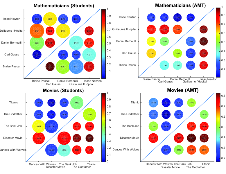
We begin our exploratory analysis by looking at some simple statistics of the data to understand the connection between choice and time. To visualize the data for each poll we use bubble plots which encode the timing and choice data for each pair of items shown to the subjects. We show the bubble plots for the student and AMT subjects for the Mathematicians and Movies polls in Figure 2. The bubble color indicates the fraction of time the item on the horizontal axis is chosen when compared to the item on the vertical axis. The size of each bubble is proportional to the average response time for each item, which is also displayed in each bubble. The bubble plots allow us to see the choice and time connection. We observe that when two items are of different qualities, i.e. one is strongly preferred to the other, the total amount of time taken to decide between them is very short. For instance, in the Mathematicians poll, for the students, it takes roughly two seconds on average to decide between Gauss and L’Hôpital, and in this pairing Gauss is chosen approximately 89% of the time. When two items are of similar qualities, the total amount of time taken to decide between them takes longer. In the Movies poll, for the students it takes 4.5 seconds on average to decide between Titanic and The Godfather, and in this pairing the Godfather is chosen approximately 41% of the time.
To make this connection between choice and time even more evident, we plot in Figure 4 the average response time versus the choice fraction (the fraction of times the less popular item is chosen) for each item pair for all polls and subjects. This restricts the choice fractions to the interval . The data for students and AMT subjects are plotted separately. As can be seen there is a clear correlation between the choice and time data for both populations. The correlation coefficient between the choice fractions and average response times is 0.84 (p-value ) for the students and 0.55 (p-value ) for the AMT subjects. This indicates that there is a clear correlation between choice and time in this data, but the strength of the correlation is different for the two populations. The students have a higher correlation between their choice and time data than the AMT subjects.
To further analyze the difference between the choice and time data for these two populations, we look at some aggregate statistics of the data. In Table 2 we list the mean choice fraction and response time (averaged across all polls and users) for the two populations. We see that on average, the response times are shorter for the AMT subjects (2.11 seconds) than for the students (3.18 seconds). For the choice fractions, a value of 0.5 would indicate random choice decisions. The mean choice fractions are closer to random for the AMT subjects (0.21) than the students (0.30). We see here that the AMT subjects have lower engagement for the poll task. They are most likely thinking less about their choices, and are therefore able to react more quickly. The students seem to be more careful in their choices, resulting in slower response times, which may be due to the fact that they were supervised by the researcher. This more careful choice decision also would explain the difference in mean choice fraction for the two populations. Recall that the choice fractions are upper bounded by 0.5, which corresponds to completely random choices. The lower mean in the choice fraction for the students comes from the fact that they give some items a lower choice fraction because they are more careful about their choices and choose certain items much less often than the AMT subjects who are choosing more randomly. This effect can also be seen in Figure 3 where we show boxplots of the choice fraction and response time for the two populations. The median choice fraction is lower and the variance is slightly higher for the students, which agrees with the engagement hypothesis. For the response times, we see that the students have a higher median and variance. This also agrees with our engagement hypothesis.
Our exploratory analysis suggests that time is not only connected to choice, but also to the level of engagement with the choice task. By not accounting for user engagement in a choice model, one could end up biasing estimates of item preferences. A choice model which captures these features could allow one to discern the interest of users in the choice decisions they make, allowing for more accurate measurement of true item preferences. This motivates our construction of a choice engagement time model in Section 4.
| Subjects | Mean choice fraction | Mean response time [seconds] | Correlation coefficient of choice fraction and mean response time |
|---|---|---|---|
| UG | 0.21 | 3.18 | 0.74 (p-value ) |
| AMT | 0.30 | 2.11 | 0.35 (p-value ) |


2.3 Comparison of Conditional Response Time Distributions
We next look at the symmetry of the timing data. In particular, we would like to know if the choice made affects the response time for a given pair of items. For instance, if comparing items and , is the response time distribution conditional on being chosen different from the reaction time distribution conditional on being chosen? For each pair of items in a poll, our null hypothesis is that these conditional distributions are equivalent and our alternative hypothesis is that they come from distributions with different medians. We test each subject population separately, as there may be different effects due to the circumstances in which the polls were taken.
For each pair of items in each poll we conducted a two-tailed Wilcox Mann-Whitney non-parametric rank sum test. This tests whether or not the two groups (choosing item or choosing item ) came from distributions with different medians. Because for each subject population we are testing multiple hypotheses (one for each item pair), to assess significance we must employ the Bonferroni correction (Dunn 1961). This corrections states that when testing hypotheses, to keep the family wide error rate (probability of making at least one type I error) at a level , one must test each individual hypothesis at a level . If any individual null hypothesis has p-value less than , then one can reject it. This corrects for the fact that with multiple hypotheses, the chance of a rare event increases and the probability of incorrectly rejecting a null hypothesis increases.
Each item pair considered corresponds to a hypothesis being tested. We can only consider item pairs where both items have at least one vote. This restriction gives us 33 item pairs for the student population and 60 item pairs for the and AMT population. We test the null hypothesis that the medians are equal at a 5% level for each subject population separately. After applying the Bonferroni correction (with for the students and for the AMT subjects) we find that we cannot reject the null hypothesis for both populations. All item pairs have p-values below the corresponding Bonferroni corrected threshold. This suggests that there may not be any difference in the distribution of the response times conditioned on the item chosen. This finding will impact the construction of our choice engagement time model in Section 4.
3 Previous Choice Time Models
Our empirical analysis has shown a relationship between choice decisions and response times. There have been different models developed to explain this phenomenon by directly modeling the mental decision process. These models were initially developed to explain the connection not between choice and time, but between accuracy and time in certain cognitive tasks. However, choice and accuracy are naturally related if one views choosing the preferred item as trying to accurately select the better item.
In this section we review the main choice time models from the psychology literature: the Poisson counter model (Pike 1973, Townsend and Ashby 1983) and the drift diffusion model (Ratcliff 1978). For each model we review the psychological assumptions underlying the model and also analyze the various predictions they make. We show that these models each possess different shortcomings. They either do not align with our empirical data or they provide computational challenges for model estimation. Our model builds upon the main properties of these models but is also relatively simple both for interpretation and estimation.
Throughout this section we assume the choice decision is made between two items and . For a given model, we let be the probability that item is chosen (and therefore is the probability that is chosen), be the average response time, and and be the average response times conditioned on or being chosen. We will investigate the predictions made for these parameters for the Poisson counter and drift diffusion models.
3.1 Poisson Counter Model
The Poisson counter model is an accumulator based choice time model where the information accumulation process is modeled as a Poisson process (Pike 1973, Townsend and Ashby 1983). In the model, there are two information accumulation processes and for the two possible responses and with rates and , respectively. These processes are modeled as Poisson processes. They accumulate information independently and in parallel. Each process has its own threshold or , respectively. The resulting choice made corresponds to the process that reaches its threshold first. The more preferred an item is, the larger the rate of its corresponding information accumulation process.
For a Poisson process with rate , the time to have arrivals has an Erlang distribution with parameters and and mean . We denote the density of an Erlang random variable as
| (3.1) |
and its corresponding cumulative distribution function (CDF) as
| (3.2) |
A choice of will be made with response time if at time has arrival and has not had arrival yet. With our notation, we can then write the joint likelihood of observing a choice and corresponding response time as
| (3.3) |
Using this likelihood function we can obtain useful properties about the Poisson counter model. For instance, the probability density function (PDF) of a response time marginalized over the choice made is simply
| (3.4) |
We plot an example of this density in Figure 5. We see two features from this plot. First, the density has a mode. Second, the tail of the density decays exponentially fast. We will come back to these properties later when we propose our choice engagement time model. In addition to the response time density, we have the following results for the Poisson counter model, which are proved in the appendix:
Theorem 3.1
For the Poisson counter model with information accumulation processes with rates and and thresholds and and for items and , respectively, we have that
| (3.5) | ||||
| (3.6) | ||||
| (3.7) | ||||
| (3.8) |
where we have defined the regularized incomplete beta function as
| (3.9) |
A natural assumption to make is that the information thresholds are equal for each item. This would correspond to a cognitive process where an item is selected when the accumulated evidence reaches a single fixed threshold. We set and and plot the resulting relationship between and as a function of in Figure 6. We see that is symmetric about and reaches its peak here. When the rates are unequal and one item is more preferred than the other, the mean response time decreases, similar to what we observed in our empirical data.
There is one property of the Poisson counter model that does not align with our empirical observations. It can easily be checked that even with symmetric thresholds, the conditional means and will be different. This lack of symmetry goes against our empirical observations. Therefore, the Poisson counter model is not the ideal model for two item choice decisions and response times.
3.2 Drift Diffusion Model
Another popular model for choice and response times is the drift diffusion model (Ratcliff 1978). Similar to the Poisson counter model, in this model when a person has to choose between items and , an information accumulation process begins. However, in this case the process is a one dimensional Brownian motion with variance , drift , and initial value . The process evolves until it hits one of two thresholds located at and . If is hit first, item is chosen, otherwise if 0 is hit first item is chosen. If is more preferred than , then will be positive with large magnitude, whereas if is more preferred than , then will be negative with large magnitude. If and are similar, then will be close to zero.
We draw upon results from the theory of Brownian motion to obtain the likelihood of the choice and response time data. We make use of the following result for hitting times of a Brownian motion.
Lemma 1 ((Feller 1959) pp. 327)
Let be a Brownian motion with drift , variance , and initial value . Let there be boundaries at and 0. Let be the density of the first time to hit 0 before hitting . Then
| (3.10) |
We note that to obtain the density of the hitting time of before 0 is hit, we simply replace by and by . With this we can easily write down the likelihood of choice and time data and as
| (3.11) |
and the density of the response time marginalized over choice is
| (3.12) |
We plot an example of this density in Figure 5. The response time density for the drift diffusion model is qualitatively similar to the Poisson counter model. For instance, it has the same uni-modal and exponential tail properties of the Poisson counter model. However, the drift diffusion model density involves an infinite sum and there can be convergence issues for small values of if not enough terms are kept in the sum, as can be seen in the figure. This can create challenges for estimating this model. Our proposed choice engagement time model will retain the qualitative properties of the response time densities, but be simple enough to enable straightforward estimation.
We can utilize standard martingale theory to obtain further properties of the drift diffusion model. We have the following results, with proof in the appendix.
Theorem 3.2
For the drift diffusion model with inital value , thresholds and for items and , drift , and variance , we have that
| (3.13) | ||||
| (3.14) | ||||
| (3.15) | ||||
| (3.16) |
As with the Poisson counter model, to gain insight into the model we focus on the symmetric case where . In Figure 6 we show the resulting relationship between and . The drift diffusion model has a natural symmetry in with respect to . Response times are short for large , which corresponds to a strong preference for one of the items. This is similar to what is seen for the Poisson counter model. However, there is a fundamental difference between the two models concerning the conditional mean response times. We have the following result, which is proved in the appendix:
Lemma 2
For the drift diffusion model with inital value , thresholds and for items and , drift , and variance , we have that .
As can be seen, unlike in the Poisson counter model, the conditional mean response times are symmetric under symmetric thresholds. This is in alignment with our empirical observations. The drift diffusion model is therefore a better model for our choice and response time data. However, it still suffers from estimation challenges due to the complexity of its likelihood function. We overcome this challenge with a simpler choice engagement time model which we propose next.
4 Choice Engagement Time Model
Our empirical analysis revealed a correlation between response time and choice and also showed the impact of user engagement on choice decisions. In this section we propose a choice engagement time model which incorporates the choice and time relationship, but also captures the user engagement phenomenon. Our model will keep the uni-modality and exponential tail of the response time density we observed for the Poisson counter and drift diffusion models. It will also possess symmetric conditional mean response times as we saw in our empirical data and in the drift diffusion model. In addition, we also want the likelihood function of the model to have a simple functional form to allow for tractable estimation. We will focus on pair-wise comparisons. That is, each choice decision will involve the user selecting the preferred item from an offer set of two items.
4.1 Basic Model
We begin by assuming that each user has a set of user specific parameters , all of which are non-negative. These parameters will govern the timing and choice behavior of the user. We assume the choice and time data to be independent conditioned on the user model parameters. For the choice data, we use a simple modification of the common Bradley-Terry choice model (Bradley and Terry 1952). We assume there is a set of items with utilities such that for . To avoid identifiably issues, we assume the normalization . Let be the choice made in the th comparison of items and by user . is one if item chosen, and zero if is chosen. We model as a Bernoulli random variable which is one with probability . Our model for incorporates the item utilities as in the traditional Bradley-Terry model, but also adds in user engagement through the parameter as follows. If items and are offered to user , then let the normalized utility of items and be and , respectively. We define and as user specific utilities for an offer set . For very large , the user specific utilities will be approximately equal to for all items. The effect of this is to reduce the difference in the items’ utility for the the user. This corresponds to a user with low engagement who sees all items as equal and chooses between them in a random manner because it does not make any difference to him which one is chosen. We let the choice probabilities be the same as in the Bradley-Terry model, but with the user specific utilities used instead of the underlying utilities, giving
| (4.1) |
The choice probability is bounded by and . For near zero the choice probability reduces to the Bradley-Terry model, but in the limit of large , the user will choose either item with probability , thereby exhibiting low engagement. Larger also results in less variation in the choice probability across item pairs.
For each choice decision we also have the corresponding response time . We model the response time as the sum of a latency time and a decision time . The latency time models how long it takes the user to view the items and recognize what they are. We model this as an exponential random variable with mean value . The decision time models how long it takes the user to decide which item to choose once he recognizes the items. Similar to the latency time, we also model this as an exponential random variable. However, for item utilities and the mean decision time is given by
| (4.2) |
and the resulting mean response time is given by
| (4.3) |
The absolute scale of the time is captured by and , both of which have units of time. The parameters and capture the user engagement. While relates uniformity of choice probability to fast response times, measures the sensitivity of the response times to the item utilities. The term is simply a regularizer that controls the mean decision time for users with high engagement. The mean response time is bounded by and . The minimum value is achieved for or equal to zero, and the maximum value is achieved for . For a user with maximum engagement ( ), the mean response time is upper bounded by . This is how the term acts to regularize the mean response time. For large , the ratio of the maximum to minimum mean response time approaches one. Therefore, for very low engagement users, there is reduced variation in the mean response time across items. This models the low engagement of the user because his response time does not depend upon the items.
The upper and lower bounds of the mean response time are set by and . However, the shape of the mean response time as a function of the item utilities is governed by . For large , is very sensitive to item utility for choice probabilities near zero or one. For small , is very sensitive to item utility for choice probabilities near one half. We show the relationship between the choice probability and mean response time in Figure 6. As can be seen, by varying we can adjust the shape of the curve. We have more flexibility with the choice engagement time model than with the drift diffusion model, but still maintain the basic symmetry of mean response time with respect to choice probability.
The response time is the sum of two exponential random variables and therefore it has a hypoexponential distribution. Formally, let be a random variable that is the sum of two exponential random variables with means and . Then is a hypoexponential random variable and we will use the convention that it is characterized by parameters and . It has mean and density
| (4.4) |
We show an example of the density of a hypoexponential response time in Figure 5. As can be seen, the shape of this density mimics that of the Poisson counter and drift diffusion models (exponential tail and a single mode), but with a much simpler functional form, allowing for more tractable model estimation.
4.2 Engagement with a No-Purchase Option
We have modeled low engagement as an increase in the randomness of user choice. However, this is not the only way engagement levels are manifested in choice and time data. For instance, we saw earlier in Tinder that low engagement users select “yes” for every match shown. This type of low engagement behavior where choices are biased against the no-purchase option can be modeled in our framework by giving every item a higher utility relative to the no-purchase option. We set the utility of the no-purchase option to . We use our existing model with every offer set containing an item and the no-purchase option. As before, we define the normalized item utilities and . The user specific utility for item is , as in the original choice engagement time model. However, for the no-purchase option we set . The no-purchase option does not gain any utility from the user’s engagement. This results in a choice probability given by
| (4.5) |
This choice probability will approach one for large , in contrast to the original choice engagement time model where the choice probability approached 1/2 for large . Therefore, for very low engagement users, each items is preferred to the no-purchase option.
In addition to preferring each item, low engagement could also result in users preferring the no-purchase option. This would occur if for some reason the users found it beneficial to reject all items. This behavior could also easily be modeled by adding to the normalized utility of the no-purchase option and leaving all other item utilities unchanged. Therefore, the choice engagement time model can capture different user engagement behaviors that may occur when the offer set is a single item and a no-purchase option.
4.3 Estimation Bias from Ignoring Engagement
In this section we study the impact of ignoring user engagement on the estimation bias of item utilities. A key benefit of modeling user engagement is that it results in more accurate estimation of item utilities by correcting for the way user engagement affects choice decisions. Ignoring user engagement will lead to biased estimates of item utilities. The amount of bias depends upon the value of the item utility and the effect can be pronounced for very popular and unpopular items.
We consider two items and with utilities and . We assume that there are users comparing the items, and each user has engagement parameter . We assume that is drawn from a distribution with mean which characterizes the engagement of the population. Each user generates a single choice decision which is one if item is chosen and zero if item is chosen. If the choice decisions are generated according to our choice engagement time model, then is a Bernoulli random variable which equals one with probability
If we neglect the user engagement, then this model reduces to the standard Bradley-Terry model.
We take a Bayesian approach and put a uniform prior on . Our estimate of when we do not account for user engagement, which we denote , will be the posterior mean. For the standard Bradley-Terry model, the posterior distribution of is a Beta distribution. If we define the statistic then the resulting posterior mean is given by
| (4.6) |
We have the following result regarding the bias of the estimator, with proof in the appendix.
Theorem 4.1
Assume choice decisions are generated according the choice engagement time model for two items with utilities and , respectively. Let the user engagement parameters be i.i.d. non-negative random variables with mean . Let be the posterior mean of in the standard Bradley-Terry model given by equation (4.6). Define
Then we have that
| (4.7) |
where the expectation is taken with respect to the user engagement parameters and the choice data.
This result shows that the bias of the standard Bradley-Terry estimate is determined by the value of and the distribution of . For the estimator is unbiased. In this case choice behavior with and without engagement are the same because the choice probabilities equal for both models. The choice data does not allow one to differentiate a choice decision between two equally preferred items or a choice decision by a low engagement user. For , the term impacts the bias. This value will be small if user engagement is large (small ). The sign of the bias depends on . For the bias is positive, which means the Bradley-Terry estimate increases the estimated utility of the item. If , then the opposite happens and the Bradley-Terry estimate decreases. Therefore, ignoring bias would increase the estimated utility of unpopular items and decrease the utility of popular items.
To further illustrate how user engagement impacts the bias, we plot in Figure 7 the estimate of the Bradley-Terry model versus the true value for for different values of . As can be seen, for lower user engagement, the bias can be significant, making one think that an item is popular when in reality it has a very low utility.
5 Model Estimation
We take a Bayesian approach to model estimation and calculate the posterior distribution of the model parameters given the observed data. We propose a hierarchical structure for the choice engagement time model which allows for the sharing of information between different users. The Bayesian approach allows for simple estimation of hierarchical models. We now provide an overview of our model specification and estimation procedure. The technical details can be found in the appendix.
5.1 Bayesian Model Specification
Our empirical data presented in Section 2 consists of choice and time data from pairwise comparisons of items in multiple polls from multiple users. For the th comparison between items and in poll by user , we denote the choice decision and response time as and . For the model parameters we impose the following structure. Item utilities are common to all users and are independent a priori. We denote the utility of item in poll as . The engagement and timing parameters are user specific, and we expect there to be some level of homogeneity in the timing behavior across users. For instance, response times on a mobile application may have a natural time scale of a few seconds for all users. To capture this shared behavior, we impose a hierarchy on the user parameters. We assume that each user parameter is drawn from a global distribution which characterizes the population. This induces a correlation among the user parameters a priori. Our model then contains user parameters which model the time and choice data generated by the users and global parameters which model the population level behavior. To specify our model we use the following notation. We let represent a normal distribution with mean and variance , represent a hypoexponential distribution with parameters and and mean (see equation (4.4)), and represent a Bernoulli distribution with mean . With this notation, our choice engagement time model specification for a user viewing items and in poll is
| (5.1) | ||||
| (5.2) |
The user parameters are given normal priors whose means and variances are given by global parameters. The priors are
The means and variances of the user parameter priors characterize the population level behavior, but still allow for flexibility to fit individual user behavior. We illustrate the structure of our choice engagement time model in the graphical model in Figure 8.
5.2 Posterior Distribution
Model estimation entails calculating the posterior distribution of the model parameters conditioned on the data. We now set up notation that will allow us to derive the form of the posterior distribution. We assume that the users are shown two items at a time. There are polls, and each poll has items. users complete all polls, and there are comparisons of items and in poll by user . In practice this value would be one, as a user would compare a pair of items once, but we allow for arbitrary values here. The model’s global parameters are the item utilities (, ) and the timing parameters . To ensure that the item utilities of each poll sum to one we set for each poll . The parameters for a user are and we define the set of all user parameters as . The observed choice and time data are and , respectively.
We start with the data likelihood. Conditioned on the user parameters, the choice and time data are independent. The choice data are Bernoulli random variables with different means and their likelihood is
| (5.3) |
where is given by equation (5.1). As shown earlier, the response times are hypoexponential random variables. We let be the probability density function of a hypoexponential random variable with parameters and given in equation (4.4). This allows us to write the likelihood of the time data as
| (5.4) |
with given by equation (5.2).
The user parameters are all normally distributed, conditioned on the global parameters. Define the normal density with mean and variance as
| (5.5) |
To simplify notation for the likelihood of the user parameters, we define the set . The the likelihood can be written as
| (5.6) |
To complete our Bayesian specification, we need to put hyperpriors on the global parameters. Following a standard Bayesian approach, we will choose uninformative hyperpriors for each parameter. We choose conjugate hyperpriors if possible to simplify the calculation of the posterior distribution. Each item utility hyperprior is a uniform distribution on . For the global means we choose normal hyperpriors with mean zero and standard deviation 100. For the global variances , we choose inverse-gamma priors with shape and scale equal to one. The inverse-gamma density with shape and scale and is given by
| (5.7) |
where is the gamma function. We denote the hyperprior distribution of the global timing parameters as and of the item utilities as . These distributions are given by
| (5.8) |
The posterior distribution for the model parameters is obtained by combining all the likelihood functions and applying Bayes rule. The resulting posterior distribution is
| (5.9) |
To evaluate the posterior distribution we generate samples form it using a Metropolis within Gibbs’ algorithm. The details of our sampling algorithm can be found in the appendix.
6 Results
We next examine the results of our Bayesian model estimation on the observed choice and time data for the student and AMT populations. We estimate the models separately for the student and AMT data in order to present the distinct behaviors of these two populations. For each population, we generated posterior samples using three independent MCMC chains with dispersed starting points run for 5000 iterations and discarded a burn-in period of 500 iterations. Convergence of the MCMC sampler was assessed using trace plots.
6.1 Student Versus AMT Subjects
The posterior means of the global model parameters for each population are shown in Table 3. Just as we found in Section 2, there is a clear difference between the student and AMT populations in terms of their timing and engagement behavior. The students have a smaller value for than the AMT population (0.20 versus 0.27) and a larger value for (1.04 versus 0.70). This indicates that the students are more engaged with their choice decisions and their response times are more sensitive to the choice decision. In fact, the difference in is quite larger, indicating that the AMT workers’ response times do not vary much as a function of the items shown. This may be due to the fact that they are online workers and may not be very diligent when making their decisions.
The estimated individual user parameters provide us more insights about the engagement of the users. We plot in Figure 9 the estimates of and for each user in the two subject populations. It can be seen that each population occupies different regions of this parameter space which correspond to their different behavioral characteristics. The student population has many users with a small and a large , whereas the AMT population has several users with a large and a smaller . There are also some users in the two populations which have similar parameter values. These users appear to have similar levels of engagement, despite being in different populations. However, overall it appears that these two subject groups exhibit different levels of engagement.
We saw earlier that the AMT subjects seemed to have lower engagement than the students. We now show that we can recover this classification using the user parameter values estimated for the choice engagement time model. We apply -means clustering with two clusters to the user parameter data. We first use as features an individual parameter, such as , or . We then try a combination of and , the features plotted in Figure 9. Finally, we include all user parameters as features. To measure the accuracy of the classification we use the average Jaccard index which is defined as follows. For two set and , their Jaccard index is defined as . This value is larger for more similar sets. We let and denote the sets of student and AMT subjects and we let and denote the two clusters produced by the -means algorithm. The average Jaccard distance is then
This measure has a maximum value of one when the sets of clusters are equal. We plot the average Jaccard index for the different feature sets in Figure 10. We see that the single feature that does best is , while combined with gives the overall best accuracy. Interestingly, when all features are used the accuracy decreases. This analysis shows the importance of for measuring engagement. While gives the influence of engagement on choice decisions, by itself it cannot separate low and high engagement users as effectively as . This may be because more engaged users will have higher variation in their response times if they have variable preferences for the items shown. The sensitivity of the response time to item preferences appears to an effective way to segment users by engagement level. While is important for correcting biases in estimating preferences, as we will see in Section 6.3, is useful for segmenting users by engagement level. Since can only be estimated from response time data, this shows the importance of response time data in choice modeling.
| Parameter | Student posterior mean (c.i.) | AMT posterior mean (c.i.) |
|---|---|---|
| [sec] | 1.37 (0.88, 1.71) | 1.18 (0.81, 1.32) |
| [sec] | 0.85 (0.64, 1.01) | 0.98 (0.89, 1.03) |
| 0.41 (0.25, 0.58) | 0.51 (0.33, 0.67) | |
| 0.20 (0.11, 0.29) | 0.27 (0.20, 0.33) | |
| 1.04 (0.71, 1.21) | 0.70 (0.56, 0.79) | |
| 0.40 (0.30, 0.55) | 0.34 (0.27, 0.42) | |
| 0.37 (0.29, 0.47) | 0.30 (0.26,0.34) | |
| 0.35 (0.27, 0.47) | 0.25 (0.20, 0.30) | |
| 0.28 (0.23, 0.34) | 0.22 (0.18,0.26) | |
| 0.47 (0.37, 0.64) | 0.37 (0.29,0.42) |
6.2 Comparison with Other Models
We next compare our model to two different benchmark models. The first model is a simple Bradley-Terry choice model where user engagement is set to zero and response times are hypoexponentially distributed with parameters and for user . We refer to this simply as a choice model. The second model, which we refer to as a choice engagement model, incorporates user engagement into the choice probability, but the response time has the same distribution as the basic choice model. We will refer to our full model as a choice engagement time model. We summarize the choice probability and mean response time for the different models in Table 4. To assess model fit, we use the deviance information criterion (DIC) (Spiegelhalter et al. 2002). This is a model fit score that favors models which fit the data well but penalizes models with many degrees of freedom. A DIC that is smaller signifies a superior model fit. We show the DIC of the three models considered in Table 4. We first see that including user engagement in the choice probability improves the model fit. Second, allowing the response times to depend upon the item utilities further improves the model fit. This shows that engagement and item dependent response times are important elements when modeling choice.
| Model | Choice probability | Mean response time | Student DIC | AMT DIC |
|---|---|---|---|---|
| Choice | 4,536 | 30,123 | ||
| Choice engagement | Equation (4.1) | 4,532 | 29,952 | |
| Choice engagement time | Equation (4.1) | Equation (4.3) | 4,435 | 29,941 |
6.3 Item Utilities
We next look at the difference in the item utilities for the different models in each population. If we do not model engagement or response times, the choice data can seem more random and items can appear to have similar utilities. When engagement and response times are included, we expect the item utilities to become more spread out and less equal. We show an example of this for the Mathematicians poll for the AMT population in Figure 11 where we plot the posterior median of the item utilities estimated from the different models. It can be seen here that when engagement is included, the utility for the most popular item increases dramatically. Without modeling engagement, one would not realize the extent to which the most popular item dominates all other items. This suggests that by modeling engagement in the choice decision, we can gain a more accurate picture of user preferences.

The divergence of the item utilities from the engagement biased values can be quantified by using the entropy measure. For a poll of items, let the utility vector be defined as with . Defined this way, the item utilities form a discrete distribution over the poll items. The entropy of this distribution is
| (6.1) |
The entropy achieves its maximum value of when all item utilities are all equal and achieves its minimum value of zero when one item has utility equal to one and all others have utility zero. High entropy corresponds to more random choices, while lower entropy corresponds to one item or a small set of items dominating the preferences. Figure 12 shows the entropy of each poll for each model and population. As can be seen, the choice model which does not model engagement always has the highest entropy. The models with engagement produce item utilities which are less uniform, resulting in a lower entropy. This effect is most dramatic for the AMT population on the Mathematicians poll, where we saw one item become completely dominant once engagement is included. The inclusion of time data slightly raises the entropy with respect to the choice engagement model for most polls, although for the student population on the Movies poll the inclusion of time data slightly reduces the entropy.
We also find that in some instances time data can also affect the resulting item utilities in significant ways. For the majority of our polls time data did not change the ranking of the items based on their estimated utilities. However, there was one poll where the inclusion of time data resulted in a change. The Movies poll for the AMT population had its top two items switched when time data was included. We show the different model rankings in the pie charts in Figure 13. As can be seen, for the choice and choice engagement models, The Godfather is the top ranked item, though only by a small amount. When time data is included in the choice engagement time model, Titanic becomes the top ranked movie, and by a wider margin. We suspect that the time data is able to discern the stronger preference of the users for Titanic, causing the resulting changing in the item ranking.
7 Conclusion
We have found that modeling engagement and response times in choice decisions can provide new insights about users’ behavior and preferences. Low engagement produces biases in choice decisions and faster response times. We saw that in certain online polls, low engagement produces random choice decisions. We also saw that there was a correlation between choice decisions and response times. We proposed a Bayesian hierarchical choice engagement time model these phenomena. Our model drew upon properties of previous psychological models, but allowed for simple estimation and interpretation. We saw that including engagement and response times in our model resulted in a better fit to observed online poll data. In addition, our choice engagement time model was able to correct for the effects of low engagement in estimating user preferences and also segment users by engagement level using estimated parameter values.
Modeling engagement and response times with choice decisions has two practical benefits. First, it provides more accurate measurements of user preferences. By not modeling engagement, one may be led to believe that certain items are equally preferred by users. However, by accounting for user engagement and response times we obtain much more asymmetric preferences which may better align with true user preferences. Second, modeling engagement and response times allows us to characterize the engagement of users at the individual level in a simple and interpretable manner. This can be of use especially to online applications which want to obtain deeper insights about their user base. For instance, users that have small and large are more engaged users who are most likely providing genuine preference data. These types of behavioral insights give online applications a more complete understanding about the true level of engagement of their user base. These insights can also help inform many operational decisions of online applications, such as choosing assortments to show users or identifying target users for marketing or promotional campaigns. Because time data is already measured in online applications, choice engagement time models can be a powerful and useful framework which can be easily implemented and utilized.
8 Appendix: Proof of Theorem 3.1
We begin by calculating , the probability that item is chosen. This is the probability that has arrivals before has arrivals, averaged over all . Another way to view this is to consider the merged process which is a Poisson process with rate . Standard results for merged Poisson processes shows that the probability of an arrival to the merged process being of type is . We want to have less than arrivals when we get arrivals. Let be the number of arrivals before arrivals. Then is a negative binomial random variable with parameters and . The CDF of a negative binomial random variable with parameters evaluated at is , where we have used the notation for the regularized incomplete beta function from equation (3.9). The probability of choosing is equal to the probability that is less than . Using the expression for the negative binomial CDF we obtain
Above we used the property .
The conditional mean response time given can be found by using the expression for the likelihood of the choice and time data given by equation (3.3). This density is defined for and . The mean response time conditional on is
| (8.1) |
Above we have used the fact that . To evaluate the integral in the above expression we make use of the following result which can be proven using elementary properties of the moment generating function of an Erlang random variable.
Lemma 3
Let be an Erlang random variable with parameters and . Then
| (8.2) |
We define to be an Erlang random variable with parameters and . Using equations (3.1) and (3.2) we have
| (8.3) |
The expectation is evaluated using Lemma 3. The expression in the summation in equation (8.3) is the probability mass function of a negative binomial random variable with parameters and . Therefore, the sum is the probability that this random variable is less than or equal to . Using the expression for the negative binomial CDF and elementary properties of the regularized incomplete beta function, we have
Inserting this into equation (8.1) we obtain our result for . To obtain , we repeat the analysis with and , and , and and all interchanged. The unconditional mean is then given by integrating equation (3.3) over and summing over , giving
9 Appendix: Proof of Theorem 3.2
Let be a Brownian motion motion with drift and standard deviation with . The probability of choosing is equal to the probability that hits before it hits 0. This can be evaluated using standard results from martingale theory. Define as a standard Brownian motion. Then . We define the stopping time . From standard results for Brownian motion we have that for any , is a martingale. We have by the optional stopping theorem that . Substituting in gives
Setting we have
We then use the fact that with probability and with probability to get
or by rearranging
The unconditional mean can be found also using martingale theory. Using our notation, . We use the fact that is a martingale and the optional stopping theorem to have . Substituting in we get
10 Proof of Lemma 2
We set and let . Applying Theorem 3.2 we have
and
Then to show the equivalence of and , we only need to show that . Using the above expression for we obtain
and
11 Proof of Theorem 4.1
The estimate of is given by . Taking the expectation of over and we have
Taking the limit as goes to infinity, we find that the bias is
12 Details of Metropolis-Within-Gibbs Sampler
We use a Metropolis-within-Gibbs scheme to sample from the posterior distribution of the model parameters. We define the set of model parameters as and for any parameter we define the set of parameters excluding as . We also define the observed choice decisions and response times as and . We must sample from the conditional distribution for each model parameter. We now derive these conditional distributions and show how to sample from them.
12.1 Global Parameters
The global parameters can be divided into to categories: means and variances. We begin the with mean parameters. For each mean parameter we use an uninformative prior distribution that is normal with mean 0 and variance . The conditional distribution of is again normal, so it can be directly sampled. We assume there are users and define . The the posterior mean and variance of are
For each variance parameter the prior distribution of is inverse-gamma with shape and scale parameters and , respectively. We can directly sample from the conditional distribution for because it is again inverse-gamma with shape parameter and scale parameter given by:
12.2 User Parameters
We now derive the conditional distribution of the user parameters. There are two categories of user parameters: those that do not directly affect the choice decision, () and those that do (). We first consider the parameters not involved in the choice decision. For each , the posterior is not conjugate so we must use a Metropolis-Hastings step. The prior distribution of is a normal distribution with mean and variance . The conditional distribution of is
where is given by equation (5.2), and is the probability density function of a hypoexponential random variable with parameters and given by equation (4.4). To sample from this conditional distribution, we use a random walk Metropolis-Hasting step. We define the th sample of as , and the proposal for sample is drawn from a normal distribution with mean and standard deviation 0.02, where 0.02 is chosen to balance the acceptance rate with step size.
The conditional distribution of is
where is given by equation (5.1), is given by equation (5.2), and is the probability density function of a hypoexponential random variable with parameters and given by equation (4.4). To sample from this conditional distribution, we use a random walk Metropolis-Hasting step. We define the th sample of as , and the proposal for sample is drawn from a normal distribution with mean and standard deviation 0.02, where 0.02 is chosen to balance the acceptance rate with step size.
12.3 Item Utilities
For each poll with items, we use the normalization . Therefore, we only need to sample for and set . We use an uninformative prior distribution for that is uniformly distributed between 0 and 1. With users’ observed data, the conditional distribution of is given by
To sample from this conditional distribution, we use a random walk Metropolis-Hasting step. We define the th sample of as , and the proposal for sample is drawn from a normal distribution with mean and standard deviation 0.02, where 0.02 is chosen to balance the acceptance rate with step size.
References
- Audley and Pike (1965) Audley, RJ, AR Pike. 1965. Some alternative stochastic models of choice. British Journal of Mathematical and Statistical Psychology 18(2) 207–225.
- Basten et al. (2010) Basten, Ulrike, Guido Biele, Hauke R Heekeren, Christian J Fiebach. 2010. How the brain integrates costs and benefits during decision making. Proceedings of the National Academy of Sciences 107(50) 21767–21772.
- Ben-Akiva and Lerman (1985) Ben-Akiva, Moshe E, Steven R Lerman. 1985. Discrete choice analysis: theory and application to travel demand, vol. 9. MIT press.
- Blanchet et al. (2016) Blanchet, Jose, Guillermo Gallego, Vineet Goyal. 2016. A markov chain approximation to choice modeling. Operations Research 64(4) 886–905.
- Bradley and Terry (1952) Bradley, Ralph Allan, Milton E Terry. 1952. Rank analysis of incomplete block designs the method of paired comparisons. Biometrika 39(3-4) 324–345.
- Chandukala et al. (2008) Chandukala, Sandeep R, Jaehwan Kim, Greg M Allenby, Thomas Otter. 2008. Choice models in marketing: Economic assumptions, challenges and trends. Now Publishers Inc.
- Debreu (1960) Debreu, Gerard. 1960. A review of individual choice behavior: A theoretical analysis. American Economic Review 50 186–188.
- Domencich and McFadden (1975) Domencich, Thomas A, Daniel McFadden. 1975. Urban Travel Demand-A Behavioral Analysis. North-Holland Publishing Company.
- Domenech and Dreher (2010) Domenech, Philippe, Jean-Claude Dreher. 2010. Decision threshold modulation in the human brain. The Journal of Neuroscience 30(43) 14305–14317.
- Dunn (1961) Dunn, Olive Jean. 1961. Multiple comparisons among means. Journal of the American Statistical Association 56(293) 52–64.
- Farias et al. (2013) Farias, Vivek F, Srikanth Jagabathula, Devavrat Shah. 2013. A nonparametric approach to modeling choice with limited data. Management Science 59(2) 305–322.
- Feller (1959) Feller, Willliam. 1959. An introduction to probability theory and its applications, second edition, vol. 1. John Wiley & Sons.
- Gallego et al. (2014) Gallego, Guillermo, Richard Ratliff, Sergey Shebalov. 2014. A general attraction model and sales-based linear program for network revenue management under customer choice. Operations Research 63(1) 212–232.
- Krajbich and Rangel (2011) Krajbich, Ian, Antonio Rangel. 2011. Multialternative drift-diffusion model predicts the relationship between visual fixations and choice in value-based decisions. Proceedings of the National Academy of Sciences 108(33) 13852–13857.
- LaBerge (1962) LaBerge, David. 1962. A recruitment theory of simple behavior. Psychometrika 27(4) 375–396.
- Laming (1968) Laming, Donald Richard John. 1968. Information theory of choice-reaction times. Academic Press.
- Leite and Ratcliff (2010) Leite, Fábio P, Roger Ratcliff. 2010. Modeling reaction time and accuracy of multiple-alternative decisions. Attention, Perception, & Psychophysics 72(1) 246–273.
- Link and Heath (1975) Link, SW, RA Heath. 1975. A sequential theory of psychological discrimination. Psychometrika 40(1) 77–105.
- McFadden et al. (1974) McFadden, Daniel, et al. 1974. Conditional logit analysis of qualitative choice behavior. Frontiers in Econometrics 105–142.
- McKeeff and Tong (2007) McKeeff, Thomas J, Frank Tong. 2007. The timing of perceptual decisions for ambiguous face stimuli in the human ventral visual cortex. Cerebral Cortex 17(3) 669–678.
- Navarro and Fuss (2009) Navarro, Daniel J, Ian G Fuss. 2009. Fast and accurate calculations for first-passage times in wiener diffusion models. Journal of Mathematical Psychology 53(4) 222–230.
- Philiastides et al. (2010) Philiastides, Marios G, Guido Biele, Hauke R Heekeren. 2010. A mechanistic account of value computation in the human brain. Proceedings of the National Academy of Sciences 107(20) 9430–9435.
- Pike (1973) Pike, Ray. 1973. Response latency models for signal detection. Psychological Review 80(1) 53.
- Ratcliff (1978) Ratcliff, Roger. 1978. A theory of memory retrieval. Psychological review 85(2) 59.
- Ratcliff (2002) Ratcliff, Roger. 2002. A diffusion model account of response time and accuracy in a brightness discrimination task: Fitting real data and failing to fit fake but plausible data. Psychonomic Bulletin & Review 9(2) 278–291.
- Ratcliff and McKoon (1997) Ratcliff, Roger, Gail McKoon. 1997. A counter model for implicit priming in perceptual word identification. Psychological review 104(2) 319.
- Ratcliff and Rouder (2000) Ratcliff, Roger, Jeffrey N Rouder. 2000. A diffusion model account of masking in two-choice letter identification. Journal of Experimental Psychology: Human perception and performance 26(1) 127.
- Smith and Vickers (1988) Smith, Philip L, Douglas Vickers. 1988. The accumulator model of two-choice discrimination. Journal of Mathematical Psychology 32(2) 135–168.
- Spiegelhalter et al. (2002) Spiegelhalter, D. J., N. G. Best, B. P. Carlin, A. van der Linde. 2002. Bayesian measures of model complexity and fit. Journal of the Royal Statistical Society 64 583–639.
- Stone (1960) Stone, Mervyn. 1960. Models for choice-reaction time. Psychometrika 25(3) 251–260.
- Talluri and Van Ryzin (2004) Talluri, Kalyan, Garrett Van Ryzin. 2004. Revenue management under a general discrete choice model of consumer behavior. Management Science 50(1) 15–33.
- TechCrunch (2015) TechCrunch. 2015. Hate it or love it, Tinder‘s right swipe limit is working. https://techcrunch.com/2015/03/12/hate-it-or-love-it-tinders-right-swipe-limit-is-working/. Accessed: 2015-11-27.
- Thurstone (1927) Thurstone, Louis L. 1927. A law of comparative judgment. Psychological review 34(4) 273.
- Townsend and Ashby (1983) Townsend, James T., F. Gregory Ashby. 1983. Stochastic modeling of elementary psychological processes. Cambridge University Press.
- Wald and Wolfowitz (1948) Wald, Abraham, Jacob Wolfowitz. 1948. Optimum character of the sequential probability ratio test. The Annals of Mathematical Statistics 326–339.