Spin pumping and measurement of spin currents in optical superlattices
Abstract
We report on the experimental implementation of a spin pump with ultracold bosonic atoms in an optical superlattice. In the limit of isolated double wells it represents a 1D dynamical version of the quantum spin Hall effect. Starting from an antiferromagnetically ordered spin chain, we periodically vary the underlying spin-dependent Hamiltonian and observe a spin current without charge transport. We demonstrate a novel detection method to measure spin currents in optical lattices via superexchange oscillations emerging after a projection onto static double wells. Furthermore, we directly verify spin transport through in-situ measurements of the spins’ center of mass displacement.
Exposing materials to strong magnetic fields has led to remarkable discoveries, most prominently the pioneering observation of the integer and fractional quantum Hall effect [1, 2]. These quantum phenomena surprise due to their robustness and independence of material properties, arising from their topological nature [3]. In this context, Thouless recognized that 1D dynamical systems can share the same topological character as the 2D integer quantum Hall (IQH) effect [4, 5]. Such topological charge pumps exhibit a quantized transport per pump cycle in a gapped filled band of an adiabatically and periodically evolving potential. More recently, a fundamentally different quantum state was observed [6], the topological insulator (TI) [7, 8], which preserves in addition to charge time-reversal symmetry. In 2D systems with spin conservation, it exhibits the quantum spin Hall (QSH) effect, characterized by a quantized spin but vanishing charge conductance. Analogous to the Thouless pump, a dynamical version of a TI can be designed – a quantum spin pump [9, 10, 11].
Spin pumps could serve as spin current sources, e.g. for spintronic applications [12]. Such spin current generators have been proposed based on the spin Hall effect [13, 14], the cyclic variation of two system parameters in interacting quantum wires [15, 16], and topological insulators [17]. However, spin pumps have been realized only in few experiments, e.g. in quantum dot structures [18] and by parametrically excited exchange magnons [19]. Here, we demonstrate the first implementation of a spin pump with ultracold bosonic atoms in optical superlattices and present a direct measurement of the arising spin current.
In 1983, Thouless investigated particle transport in two superimposed 1D periodic potentials adiabatically moved relative to each other . This sliding motion periodically varies the combined potential and thereby the underlying single-particle Hamiltonian, which can be parametrized by the cyclic pump parameter . During the pumping, a particle acquires an anomalous velocity proportional to the Berry curvature defined on the closed surface spanned by and the quasi-momentum . The resulting displacement after one pump cycle only depends on the geometric properties of the pump cycle and is not quantized unless all quasi-momenta of a band are occupied equally. In this case, the pump is topological with a displacement proportional to the Chern number, the integral of the Berry curvature over the entire surface. Thus, transport is quantized and robust against perturbations [4, 5]. Recently, such geometric and quantized, topological pumps have been realized with ultracold bosonic [20, 21] and fermionic atoms [22].
In analogy to the Thouless pump, a spin pump can be thought of as a dynamical version of a QSH system [9], which is characterized by a bulk excitation gap and gapless edge excitations. In general, the electron spin is not conserved, e.g. in the presence of spin-orbit coupling, and therefore unconventional topological invariants, like the index [7], are needed for classification. Non-interacting QSH systems with spin conservation can be interpreted as two independent IQH systems. Therefore, a quantum spin pump can be composed of two independent pumps, where the up and down spins have inverted Berry curvature and are therefore transported in opposite directions.
A quantum spin pump can be implemented with ultracold atoms in two hyperfine states in a spin-dependent dynamically controlled optical superlattice, which can be formed by superimposing two lattices with periods and . In the tight binding limit, a spin in this superlattice is described by the Rice-Mele model [23], which comprises staggered on-site energies between neighboring sites and alternating tunnel couplings with the dimerization parameter . Pumping can be induced by an adiabatic modulation of the potential and corresponds to a loop in parameter space (, ) around the degeneracy point (, ). If the two spin components do not interact with each other, their pumping motion is independent and a spin pump can be realized by a spin-dependent deformation of the potential, so that time-reversal symmetry is retained and their Berry curvature is reversed. The associated spin transport is quantized only for equal occupation of all quasi-momenta, which can be realized with non-interacting fermions by placing the Fermi energy in the band gap and bosons by localizing each spin component to a Mott insulator with negligible inter-spin interaction.
In addition, the two spin components can be coupled by introducing on-site interactions between the atoms. For hardcore interactions and unit filling, the bare tunneling is suppressed and the system can be described by a 1D spin chain
| (1) | ||||
with spin-dependent tilt and alternating exchange coupling . For large tilts the many-body ground state are locked spins in an antiferromagnetic order, while for strong exchange coupling dimerized entangled pairs are favored. Implementing this Hamiltonian requires a dynamically controllable spin-dependent superlattice [24, 25]. In the limit of isolated double wells , applying a global gradient to a spin-independent superlattice can locally reproduce the staggered tilts (Fig. 1(a)). In this situation, a variation of the parameters (, ) during the spin pump cycle corresponds to a modulation of (, ) in the interacting 1D spin chain. This cycle needs to be performed adiabatically with respect to the intra double well exchange coupling . The pump cycle encircles the degeneracy point (, ) as illustrated in Fig. 1(a). Despite the antiferromagnetically ordered state being an excited many-body state in the globally tilted system, the pump can still be described by a topological invariant as the pump of Eq. 1 with local tilts, if the pumping is fast compared to , which determines the gaps of additional level crossings in the spectrum [26]. This can be readily achieved in the experiment by choosing lattice depths, for which inter-double well coupling is quenched.

The experimental setup consists of a 3D optical lattice with a superlattice along the -axis and deep transverse lattices along and to create an array of decoupled 1D systems. Each system is initially occupied by an antiferromagnetically ordered spin chain of up and down 87Rb atoms [27], localized on individual sites with [26]. To start the pump cycle, every second barrier is decreased to transfer two neighboring spins to the ground state of a double well. Since a large magnetic gradient is present along , the up (down) spin stays localized on the left (right) side, shortly denoted as . The gradient is then reversed adiabatically compared to . Thereby the wavefunction follows the instantaneous eigenstate and a spin current occurs as the two spins exchange their positions via the delocalized triplet state at (Fig. 1(b)). At the end of the first half cycle, individual sites are decoupled by increasing the short lattice depth. Subsequently, is inverted by flipping the dimerization and also the magnetic gradient to maintain the correct local tilts (insets Fig. 1(a)). This corresponds to a projection on double wells shifted by one lattice site. The state of the system remains unchanged during this sudden switch and the spins in the new shifted double well are in the ground state. After a full cycle, the two spin components have each moved by in opposite directions; therefore the total particle current vanishes as the contributions from the two spin components cancel each other exactly. Thus, pumping leads to a spin transport without inducing a particle current.
The spin current between the left (L) and the right (R) site of a double well is related to the change in the expectation value of the spin imbalance given by the integral form of the continuity equation , with the occupation of spin on site . To understand how this spin current arises and how it can be detected, it is useful to examine the evolution of the eigenstates during the adiabatic change of . Two spins initially at time in the eigenstate of the two-particle double well Hamiltonian [26] follow the instantaneous eigenstate , but acquire – even for a perfect adiabatic evolution – a small imaginary contribution from other eigenstates . This admixture occurs only temporarily during the ramp and induces an anomalous spin velocity (Fig. 2(a)). The coefficients can be calculated in first-order perturbation theory with the ramp speed and the eigenenergy of [28]. When starting from the ground state , the wavefunction is well approximated by only considering contributions from the first excited state . The -coefficients of higher lying states are strongly suppressed as the corresponding wavefunctions depend weakly on and . The wavefunction can be probed by a sudden stop of the pump cycle at time by projecting it onto . During the subsequent time evolution, the two states and acquire a relative phase leading to oscillations of the spin imbalance with the imbalance at time . The oscillation amplitude is proportional to the admixture of the second eigenstate and can be related to the spin current through the continuity equation [26]
| (2) |
Experimentally, the gradient ramp was abruptly stopped at and a time trace of the resulting double well superexchange oscillation [29] was recorded by a simultaneous measurement of , , and with Stern-Gerlach separated site-resolved band mapping images (Fig. 2(a)). The amplitude was found by fitting
| (3) |
to the oscillation data, where and a phase shift induced by a finite freezing ramp speed. Compared to the ideal evolution, two additional effects are taken into account. First, an exponential decay of the amplitude with a time constant accounts for dephasing between individual double wells. Both, and the oscillation frequency were determined for each with an independent superexchange oscillation measurement. Second, an additional decay of the imbalance offset is caused by an exponential relaxation of a small residual magnetic field gradient after the abrupt stop of , with a decay constant . The resulting oscillation amplitudes during the pump cycle for two different as well as exemplary spin imbalance traces are summarized in Fig. 2(b). The spin current peaks around , where the ground state is delocalized and spins move. For large gradients the eigenstates are independent of and the spin current vanishes. Note that the residual gradient slightly shifts the peak towards higher . Furthermore, the spin current strongly depends on the exchange coupling . With increasing , the wavefunction delocalizes and depends less on , so the peak width increases while the maximum amplitude decreases. However, unlike the instantaneous current, the transported spin during one pump cycle, is independent of the pump parameters.

To compare the data with theoretical expectations, we performed a numerical calculation including a reduced detection efficiency caused by the residual gradient decay. Imbalance time traces for were evaluated using a two spin, two-site extended Bose-Hubbard Hamiltonian with [30, 26]. The calculated time traces were also fitted with Eq. 3; the resulting oscillation amplitude describes ideal transport of ground state spins (light lines in Fig. 2). This curve can be fitted to the data by rescaling the amplitude with a factor of , which directly determines the reduction of the integrated measured current compared to the ideal one and thereby the transported spin polarization. The deviation from ideal transport can be attributed to an imperfect initial state preparation with ground state occupation and a pump efficiency per half a pump cycle of , which describes the fraction of double wells that remain in the ground state after half a cycle. Considering this additional occupation of the first excited state, which creates an opposite current, the total spin current can be calculated (dark lines in Fig. 2(b)). Fitting these expected oscillation amplitudes to the measured data by rescaling with a global factor results in a fit value of for and for . This shows that even though the shape and amplitude of the curve changes, the integrated current is only defined by the pumps’ topology not by the specific tunneling parameters. Furthermore, we note that the deviation to the theoretically expected integrated current can not be attributed to edge effects as they are negligibly small for the present trapping potential.
To study the dependence of the maximum current on the exchange coupling, the oscillation amplitude was measured at for various (Fig. 3). The maximum amplitude decreases with rising , as the spins’ wavefunction is more delocalized for the same and therefore the current flow is spread over a larger sector in the pump cycle. The observed peak amplitude agrees with the numerical model including the initial ground state occupation and pump efficiency. As suggested by the measurements in Fig. 2, the integrated spin current can be extracted by rescaling the ideal amplitude with a global factor and is found to be constant for all exchange couplings (inset Fig. 3).
Independent evidence for the spin separation and a quantitative comparison with the total spin current can be obtained by measuring the center-of-mass position of the two spin components from in-situ absorption images after removing one of the spin components. When varying , the up and down spins clearly separate (Fig. 4). This independently verifies the spin transport and shows quantitative agreement with the results of the spin current measurement [26].
In conclusion, we have demonstrated the implementation of a spin pump and introduced a new method for directly measuring instantaneous spin currents. Comparing the measured spin imbalance oscillation amplitudes with the adiabatic theory shows that the integrated current is independent of the specific pump parameters and gives evidence for the utility of the developed current measurement method. The method can also be extended to more general systems by performing an instantaneous projection onto double wells. Investigating such spin pumps on a single site level would allow for local observation of spin currents and the direct observation of edge excitations in finite systems [31]. A system described by the non-trivial -invariant can be realized with time-reversal invariant spin orbit interaction [9, 11]. When breaking time-reversal symmetry, the topological properties of the QSH system remain but spin-Chern numbers are required for the description [11]. Furthermore, a topological, interaction-driven quantum motor [32, 33] can be accomplished by only pumping one of the components while the other is coupled by interaction. For spin pumps with highly degenerate many-body ground states, fractional transport is predicted [34].
We acknowledge insightful discussions with M. Aidelsburger. This work was supported by NIM, the EU (UQUAM, SIQS), and the DFG (DIP & FOR2414). M. L. was additionally supported by ExQM and R. C. by FIRB-2012-HybridNanoDev (Grant No. RBFR1236VV).
References
- [1] K. v. Klitzing, G. Dorda, and M. Pepper, Phys. Rev. Lett. 45, 494 (1980).
- [2] D. C. Tsui, H. L. Stormer, and A. C. Gossard, Phys. Rev. Lett. 48, 1559 (1982).
- [3] D. J. Thouless, M. Kohmoto, M. P. Nightingale, and M. den Nijs, Phys. Rev. Lett. 49, 405 (1982).
- [4] D. J. Thouless, Phys. Rev. B 27, 6083 (1983).
- [5] Q. Niu and D. J. Thouless, J. Phys. A 17, 2453 (1984).
- [6] M. König, S. Wiedmann, C. Brüne, et al., Science 318, 766 (2007).
- [7] C. L. Kane and E. J. Mele, Phys. Rev. Lett. 95, 226801 (2005).
- [8] B. A. Bernevig and S.-C. Zhang, Phys. Rev. Lett. 96, 106802 (2006).
- [9] R. Shindou, J. Phys. Soc. Jpn. 74, 1214 (2005).
- [10] L. Fu and C. L. Kane, Phys. Rev. B 74, 195312 (2006).
- [11] C. Q. Zhou, Y. F. Zhang, L. Sheng, et al., Phys. Rev. B 90, 085133 (2014).
- [12] G. A. Prinz, Science 282, 1660 (1998).
- [13] S. Murakami, N. Nagaosa, and S.-C. Zhang, Science 301, 1348 (2003).
- [14] Y. K. Kato, R. C. Myers, A. C. Gossard, and D. D. Awschalom, Science 306, 1910 (2004).
- [15] P. Sharma and C. Chamon, Phys. Rev. Lett. 87, 096401 (2001).
- [16] R. Citro, N. Andrei, and Q. Niu, Phys. Rev. B 68, 165312 (2003).
- [17] R. Citro, F. Romeo, and N. Andrei, Phys. Rev. B 84, 161301 (2011).
- [18] S. K. Watson, R. M. Potok, C. M. Marcus, and V. Umansky, Phys. Rev. Lett. 91, 258301 (2003).
- [19] C. W. Sandweg, Y. Kajiwara, A. V. Chumak, et al., Phys. Rev. Lett. 106, 216601 (2011).
- [20] M. Lohse, C. Schweizer, O. Zilberberg, M. Aidelsburger, and I. Bloch, Nat. Phys. 12, 350 (2016).
- [21] H.-I. Lu, M. Schemmer, L. M. Aycock, et al., Phys. Rev. Lett. 116, 200402 (2016).
- [22] S. Nakajima, T. Tomita, S. Taie, et al., Nat Phys 12, 296 (2016).
- [23] M. J. Rice and E. J. Mele, Phys. Rev. Lett. 49, 1455 (1982).
- [24] P. J. Lee, M. Anderlini, B. L. Brown, et al., Phys. Rev. Lett. 99, 020402 (2007).
- [25] H.-N. Dai, B. Yang, A. Reingruber, et al., Nat. Phys. 12, 783 (2016), article.
- [26] See Supplemental Material.
- [27] A. Widera, F. Gerbier, S. Fölling, et al., Phys. Rev. Lett. 95, 190405 (2005).
- [28] D. Xiao, M.-C. Chang, and Q. Niu, Rev. Mod. Phys. 82, 1959 (2010).
- [29] S. Trotzky, P. Cheinet, S. Fölling, et al., Science 319, 295 (2008).
- [30] V. W. Scarola and S. Das Sarma, Phys. Rev. Lett. 95, 033003 (2005).
- [31] Y. Hatsugai and T. Fukui, Phys. Rev. B 94, 041102 (2016).
- [32] F. Zhou, Phys. Rev. B 70, 125321 (2004).
- [33] R. Bustos-Marún, G. Refael, and F. von Oppen, Phys. Rev. Lett. 111, 060802 (2013).
- [34] D. Meidan, T. Micklitz, and P. W. Brouwer, Phys. Rev. B 84, 075325 (2011).
Supplemental Material for:
Spin pumping and measurement of spin currents in optical superlattices
C. Schweizer1,2, M. Lohse1,2, R. Citro3,4, I. Bloch1,2
1 Fakultät für Physik, Ludwig-Maximilians-Universität, Schellingstrasse 4, D-80799 München, Germany
2 Max-Planck-Institut für Quantenoptik, Hans-Kopfermann-Strasse 1, D-85748 Garching, Germany
3 Dipartimento di Fisica “E. R. Caianiello”, Università degli Studi di Salerno,
Via Giovanni Paolo II 132, I-84084 Fisciano (Salerno), Italy
4 SPIN-CNR Salerno, Via Giovanni Paolo II 132, I-84084 Fisciano (Salerno), Italy
S.XII Spin current measurement
S.XII.1 Two-site extended Bose-Hubbard model
In the tight binding limit, two spins on an isolated double well () can be described by a two-site Bose-Hubbard model, where we denote the spins and the left (right) site with L (R). The Hamiltonian is given by
| (S.1) | ||||
with () the creation (annihilation) operator of spin on the left or right site, the number operator counting the spins, the tunneling rate, the spin-dependent energy offset between left and right site, and the on-site interaction energy. The accuracy of the exchange coupling, especially at large , can be increased by including corrections from density-dependent hopping and nearest neighbor interaction [1, 2]. Here, denotes the Wannier function on the left/right site. The Hamiltonian of this extended Bose-Hubbard model is in the basis , , , with :
| (S.2) |
The dependence of the energy spectrum of the extended Bose-Hubbard model on is shown in Fig. S1(a). We define the exchange coupling as the gap between the first and second eigenenergy at . The ground state in the limit is for positive and for negative . At and the ground state is approximately a triplet state . Note that the third eigenstate is independent of .
An adiabatic change of the tilt with rate leads in first-order approximation to the temporary wavefunction
| (S.3) |
using parallel transport conditions [3]. Here, is an instantaneous eigenstate of and the admixture coefficients are
| (S.4) |
A detailed derivation can be e.g. found in Ref. [3]. The -coefficients for , i.e. starting from the ground state, are depicted in Fig. S1(b); the contribution clearly dominates and other coefficients can be neglected because the dependence of the eigenstates and on is weak or even vanishing because of the large gap , for . Then the temporary wavefunction Eq. S.3 reduces to
| (S.5) |
S.XII.2 Connection Between Amplitude and Current
For the current measurement, the pump cycle is abruptly stopped at . In the ideal case this happens instantaneously, such that the wavefunction subsequently evolves according to the static Hamiltonian . Since is in general not an eigenstate of , the expectation value of the imbalance operator oscillates in time
| (S.6) |
with . The oscillation amplitude is directly proportional to the -coefficient
| (S.7) |
When comparing this result to the the integral form of the continuity equation, the spin current at is directly connected to the oscillation amplitude via
| (S.8) | ||||
S.XII.3 Oscillation Amplitude – Model and Corrections
For two spins occupying the ground state of an isolated double well, the ideal oscillation amplitude for a perfectly abrupt stop of the ramp can be evaluated from Eq. S.7. This ideal amplitude, within , is shown as a function of in Fig. S2 (green solid lines). As the abrupt stop is smoothed by a decaying residual magnetic gradient, the measured amplitude for a given spin current is slightly reduced. This amplitude can be calculated numerically by solving the time-dependent Schrödinger equation including the residual magnetic gradient decay. The model assumes an initial state after the adiabatic evolution (Eq. S.5) stopped at and a time-dependent Hamiltonian . For long times , the Hamiltonian approaches the ideal case. With a numerical time propagation, the evolution of the wavefunction and thereby can be calculated. From this time trace the amplitude is extracted with a fit of 3 from the main text as for the experimental data. The effect of this detection correction is visualized in Fig. S2 as orange solid lines.
Preparing only ground state double wells is extremely challenging and therefore a small residual amount of excited state double wells is expected. When considering only ground and first excited state, the spin imbalance is a good measure for the state occupation at , where the spins are perfectly localized. By measuring the spin imbalance before () and after half a pump cycle (), the initial state preparation and the pump efficiency can be characterized. The pump efficiency is a measure of the fraction of double wells that remain in the ground state during half a pump cycle and can be deduced from the spin imbalance: . The initial fraction of ground and excited state double wells is and , assuming being the ideal spin imbalance at the initial conditions.
The integrated spin current is the sum of the ideal integrated spin currents of both states weighted by the initial band occupation and the pump efficiency. The ideal spin currents are oppositely directed and given by the ideal initial spin imbalance. Furthermore, equal pump efficiency for ground and first excited state are assumed.
| (S.9) | ||||
The result can be verified by a comparison with the integral form of the continuity equation .
The reduction of the integrated current as a result of a finite excited state occupation and a reduced pump efficiency can be approximately captured in the data analysis by rescaling of the current with a global factor. Such a rescaling corresponds to a description by an average state occupation with perfect pump efficiency. The blue line in Fig. S2 shows the spin current taking into account the detection efficiency, the initial ground state occupation as well as the pump efficiency.
S.XIII Energy spectrum
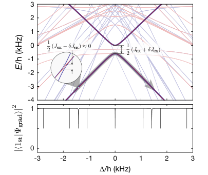
In the experiment, the spin chain with local tilts is realized in the limit of isolated double wells with a global magnetic gradient. In this system unlike for in 1 of the main text, the prepared initial state is not the ground state but an excited state. During the pump cycle, however, it evolves in the same way as the ground state of a spin-dependent superlattice with the exception of a number of additional crossings that occur in the energy spectrum (see Fig. S3). However, the gaps are very small – on the order of the inter double well exchange coupling – and can be crossed non-adiabatically. In conclusion the gradient model requires not only adiabaticity with respect to the intra double well exchange tunneling but also pure non-adiabatic transfer with respect to gaps on the order of the inter double well exchange coupling . As the latter can be suppressed exponentially with the long lattice depth, and adiabaticity on the double well scale can be reached by slower ramp speed, the transport in these models can be described by the same topological invariant. An energy spectrum for two up and two down spins on two double wells is shown in Fig. S3 for the experimental parameter set for . The pump cycle follows the thicker darker depicted state, which is either strongly gapped around or crosses states with negligibly small gaps. Additionally, the state overlap between the groundstate in the staggered model and the pumped state for the model with a global gradient is calculated and found to be one, apart from the vicinity of the tiny gaps. This shows that the pumped state in the gradient model is very similar to the one in the model with staggered tilts.
S.XIV Experimental sequence
The experimental sequence starts with a Mott insulator of 87Rb atoms in a 3D optical lattice of three mutually orthogonal standing waves with wavelengths nm and nm. With a sequence of microwave driven adiabatic passages, the atoms are transferred to the via the state (see , in Fig. S4). Then two neighboring lattice sites are merged along the -direction into decoupled sites with twice the period by ramping up a long lattice with period , where , and simultaneously turning the short period lattice off. With coherent microwave-mediated spin changing collisions [4] each atom pair is transferred to a pair of and atoms. Subsequently, a magnetic field gradient is turned on and the long lattice sites are split adiabatically into two decoupled sites by turning on the short period lattice to a depth of in ms with , where is the mass of a Rubidium atom. Due to the present magnetic field gradient of kHz during the splitting, the up and down spins order antiferromagnetically in individual, decoupled sites with . A detailed time sequence of the individual experimental parameters is shown in Fig. S4(a). This initial state preparation is then followed by the pumping sequence.
The spin pump sequence for multiple cycles, which was used for the in-situ measurements, starts by coupling neighboring lattice sites of each double well by decreasing the short period lattice to the final value for the corresponding superexchange coupling. Then, the spin-dependent gradient is inverted adiabatically by changing the bias field along the -direction (see gradient calibration), and at the end of the first half pump cycle the distribution is frozen again by increasing the short lattice depth such that . To continue the cycle, the dimerization is changed by swapping to a second laser which creates a -shifted long lattice, and simultaneously setting the magnetic bias field back to its initial value in . Then the previously described cycle is repeated multiple times. Before in-situ imaging, residual atoms in the (, ) state are removed by applying simultaneously a microwave field on the (, )(, ) transition and a resonant imaging light pulse to remove the atoms in the manifold. Subsequently, one of the spin states is selected and transferred to the (, ) state by a microwave driven adiabatic passage and imaged by absorption imaging.
The current measurement sequence is limited to the first half pump cycle. Neighboring sites are coupled by decreasing the short lattice depth and the bias field is changed with a constant rate to different final values of the magnetic tilt , where it is abruptly stopped. After a variable holdtime , the spin distribution is frozen by ramping up the short period lattice and a site-resolved band mapping was performed. During time-of-flight, the spin-components are separated spatially by a Stern-Gerlach field and the four site occupations , , , and can be simultaneously extracted from each absorption image.
S.XV Calibration of lattice, gradient field and Hubbard parameters
Calibration of bare tunneling rate:
The bare tunneling matrix element couples two neighboring sites and can be calibrated from left-right oscillations of a single atom on a double well with degenerate on-site energies (). At the beginning, a single atom is prepared on the left site of each double well. To this end, an Mott insulator in the long lattice is prepared and adiabatically split with the short lattice in the presence of a large potential tilt. The short lattice depth is increased such that the atoms localize on the lower-lying left site (). Then, the tilt is removed and subsequently the short period lattice is ramped down in to the lattice depth at which needs to be calibrated. The localized wavefunction is not an eigenstate of the symmetric double well, but an equal superposition of the ground and first excited state and thus the left-right occupation oscillates in time. The left-right fraction can be measured with site-resolved band mapping and its oscillation frequency is equal to the difference of the single-particle eigenenergies .
Calibration of on-site interaction energy:
The on-site interaction energy is the extra energy for placing a second particle on the same site and can be calibrated via the superexchange oscillation frequency. An up and a down spin are localized on the left and right site of a double well prepared in the presence of a large spin-dependent tilt as for the current measurement. Then, the magnetic fields, except for a small bias field to maintain the quantization axis, are switched off to non-adiabatically remove the tilt while and afterwards the short period lattice is decreased within to the final value, at which is calibrated. The localized state is not an eigenstate anymore and evolves in time. The time evolution leads to superexchange oscillations [2], which for the experimentally used parameters are dominated by the contributions from the ground and first excited state . The exchange coupling can be calculated from an extended Bose-Hubbard model and depends strongly on . Thus, can be inferred from .
Gradient Calibration:
The spin-dependent gradient field is generated by two pairs of coils: an anti-Helmholtz pair along the -direction, which creates a quadrupole field , and a Helmholtz pair along the -direction, which creates a homogenous bias field with the unit vector in -direction. At the atom cloud (), the total magnetic field is and the magnetic field gradient depends linearly on the bias field for . A precise knowledge of the spin-dependent double well tilt is required for the current measurement method. To this end, a calibration was performed using laser-assisted tunneling spectroscopy. The setup comprises two beams interfered under an angle of with a frequency difference of forming a running wave lattice oriented at to the physical lattice. A single spin in the (, )-state is loaded in the ground state of a tilted double well potential with and additional magnetic tilt , which needs to be calibrated. The running wave lattice modulates neighboring lattice sites relative to each other and will induce tunneling if . A series of spectroscopy scans varying are performed for various magnetic field values . The resulting data is shown in Fig. S5. For large a deviation from the linear behavior is visible, which can be captured by fitting the magnetic field distribution of a quadrupole field
| (S.10) |
where both and are fit variables.
Decay Calibration:
During the current measurement sequence, the magnetic field gradient is ramped to a final value and abruptly stopped there. Experimentally, an instantaneous stop is not realizable but a small residual gradient remains which decays slowly during the current measurement. The calibration of the decay time as well as the residual gradient at is essential for the current measurement and is realized with microwave spectroscopy. The sequence starts with a single spin in the (, ) state localized on the left site by a strong magnetic gradient. The gradient is reduced with the identical rate as for the current measurement and stopped at but individual sites are decoupled by a large short lattice depth. Now, resonance frequency scans on the (, )(, ) microwave transition with a pulse duration of are recorded at various times around ; the gradient determined from the center frequencies is summarized in Fig. S6. A clear exponential decay can be fitted for with a decay constant . The amplitude can be calibrated by comparing the linear increase for with the gradient calibration (Fig. S5) and leads to for sites separated by . This corresponds to a tilt in the superlattice for the experimental parameters of at and at . The difference originates mainly in the slightly different distance between the sites depending on the double well parameters.
Simultaneous band mapping of two spins:
The simultaneous site-resolved detection of two spins per double well suffers from an additional reduction of the detected imbalance. This reduction occurs during the merging of the left and right site of each double well in the presence of a spin-independent tilt into a single site of the long lattice. This process transfers atoms from the left site to the ground band and spins from the right site to the second excited band of the long lattice. The subsequent band mapping measures the band occupation and hence also the site occupations. However, spins in these bands undergo singlet-triplet oscillations after and also during the merging [5, 2]. A calibrated holdtime before the release is chosen such that correct imbalances are detected. Nevertheless, the detected imbalance is reduced most likely due to dephasing during the merging ramps. The value of this reduction can be calibrated to rescale the measured imbalances with a constant factor to correctly determine the imbalance. The calibration measurement compares the two spin site-resolved band mapping with a single spin band mapping, where shortly before the merging one of the spin components is removed by an adiabatic spin transfer and a subsequent resonant light pulse.
S.XVI Multiple pump cycles
S.XVI.1 Band mapping data
The in-situ data show a separation and opposite transport of the two spin components for multiple pump cycles. In Fig. S7 the spin imbalance during the pump cycle is depicted versus the pump parameter , which is defined as the angle of the pump path in parameter space . The imbalance starts with a negative value, the state is predominantly , and inverts during the first half pump cycle. After switching the dimerization, the pump cycle continues by inverting the spin-imbalance each half pump cycle. At a small step in is visible, which originates mainly from singly occupied sites created at the surface of the atom cloud during pumping.
S.XVI.2 Initial state and pump efficiency
For the in-situ measurement the calculated motion of a localized spin is shown, which takes into account the initial ground state occupation and pump efficiency per -th half pump cycle. The model is analogous to the one for the spin current, where the corrections are extracted from the spin-imbalance measured at each half pump cycle. The step height is then given by
| (S.11) |
with and . In total, the displacement after the -th half pump cycle is
| (S.12) |
S.XVII Pump scheme in a tight-binding model with magnetic field gradient
In the tight-binding approximation the dynamics of non-interacting atoms in an optical superlattice potential in the presence of a field gradient is described by a generalized Harper model with a site-dependent Zeeman-like term
| (S.13) | ||||
with . The pumping scheme is implemented with a cycle, in which and where the pump parameter changes constantly in time . In the deep tight-binding regime the parameter space describes an ellipse . At , the spectrum has an energy gap , and thus the adiabatic condition is met if .
The part of the Hamiltonian is odd while the part is even under time-reversal symmetry and therefore Eq. S.13 belongs to the class that satisfy the condition , where is the time-reversal operator. Moreover, the Hamiltonian is time-reversal invariant at two points and , where dominates. The existence of these two points plays a crucial role in the classification of the pump cycle. In particular, pump cycles in which and have different time reversal polarization are topologically distinct from trivial cycles and define a spin-pump. In a single double well at time , dominates and locks the up (down) spins on the left (right) well, denoted by . This state evolves into the state after half a pump cycle at , where the two spins have exchanged their positions. In contrast, at and , the term dominates and the spins are delocalized over the double wells; then the system is dimerized.
S.XVIII Center of mass shift and time-reversal polarization
Consider a Hamiltonian Eq. S.13 with lattice constant and periodic boundary conditions. Then, in absence of spin-orbit type of interaction that means independent spin components without inter-spin interactions, the spin transport for a homogeneously populated band is characterized by the spin Chern number . Since the spin components are decoupled even in the presence of a field gradient, the Chern numbers can be evaluated using the Thouless-Kohmoto-Nightingale-Nijs expression [6]:
| (S.14) |
where is the Berry curvature associated to the single-particle wavefunction
| (S.15) |
The spin Chern number can be furthermore related for the non-interacting case to the topological invariant that distinguishes a nontrivial pump from a trivial one and is related to the change in time reversal polarization.
As known from polarization theory [7], the charge polarization is the center of mass of a localized Wannier state and is in turn related to Berry’s phase of the corresponding Bloch functions. In the same way, the polarization of a single spin component is given by:
| (S.16) |
where is the Berry connection. The change in polarization induced by changing the pump parameter by , or the time variable, corresponds to the Chern number [7]
| (S.17) |
The spin-density can be directly measured by in-situ absorption imaging for a single spin component. The change of spin-polarization at two different times and , coincides with the spatial shift of the Wannier function. Measuring the center of mass shift for a single spin component thus gives the Chern number of this component.
For time-reversal invariant systems, taking into account the role of Kramer’s degeneracy, one can define a corresponding time-reversal polarization in terms of the difference of the individual spin polarizations . Hence, the change in time-reversal polarization during a cycle gives the topological invariant. Furthermore, it is equal to the integration of the instantaneous spin-current over the pump cycle as, .
S.XIX Spin pumping with interactions
When in addition hardcore interactions between the spin components are assumed, spin pumping can be understood in a similar way as in the non-interacting case. For half filling a representation in terms of spin operators can be introduced in this limit:
| (S.18) | ||||
Model Eq. S.13 can thus be mapped to a model of an antiferromagnetic spin chain with two perturbations
| (S.19) | ||||
where the second term describes a staggered component of the exchange interaction, while the last one is a Zeeman-like term, which controls the on-site energies.
A cycle, in which are adiabatically varied defines a topological spin pump [8]. Such a spin pump transfers per cycle, which can be still described by the topological invariant. Note that the Hamiltonian in Eq. S.19 corresponds to a cosine band . The staggered exchange interaction opens a gap at and for half filling, only the lowest subband is occupied. Due to the periodicity in -space, the double degenerate point is identical to that at and becomes the source and sink for a vector field and defined in the --parameter space. If a pump path encloses the origin , e.g. , where , the number of lattice sites that a spin is transported, is given by the flux enclosed by the path
| (S.20) |
This corresponds to a quantized spin transport. The total at one end of this system increases while that at the other end decreases by one during the entire cycle as long as the gap is maintained open and the point is not outside the 2D closed surface.
Away from the hard-core constraints for the bosons, the effect of a finite interaction can be taken into account via a bosonization approach. When applying Haldane’s bosonization of interacting bosons [9] to the Hamiltonian Eq. S.13 and , the Hamiltonian of the bosons can be written as:
| (S.21) |
where the two canonical fields fulfill , is the velocity of excitations, and is the Tomonaga-Luttinger exponent. In the case of hard-core bosons, and , while is the boson density.
Introducing the fields , the boson annihilation operators can be represented as [9]:
| (S.22) | ||||
where are non-universal coefficients. For hardcore bosons at half filling, these coefficients have been found analytically [10]. From Eq. S.22, the bosonized expression of the staggered hopping term can be deduced:
| (S.23) |
with only the most relevant term in the renormalization group sense and the charge and spin variables . When is pinned (e.g. at commensurate fillings) in the gapped spin phase also the field is pinned . The excitations above the ground state are solitons and antisolitons, which are topological excitations of the field that carry a spin .
The time reversal-polarization is identified as and because under time reversal , time reversal polarization is either or . Thus, the topological classification of the spin pump remains also away from the hard-core bosons limit.
References
- [1] V. W. Scarola and S. Das Sarma, Phys. Rev. Lett. 95, 033003 (2005).
- [2] S. Trotzky, P. Cheinet, S. Fölling, et al., Science 319, 295 (2008).
- [3] D. Xiao, M.-C. Chang, and Q. Niu, Rev. Mod. Phys. 82, 1959 (2010).
- [4] A. Widera, F. Gerbier, S. Fölling, et al., Phys. Rev. Lett. 95, 190405 (2005).
- [5] M. Anderlini, P. J. Lee, B. L. Brown, et al., Nature 448, 452 (2007).
- [6] D. J. Thouless, M. Kohmoto, M. P. Nightingale, and M. den Nijs, Phys. Rev. Lett. 49, 405 (1982).
- [7] N. Marzari and D. Vanderbilt, Phys. Rev. B 56, 12847 (1997).
- [8] R. Shindou, J. Phys. Soc. Jpn. 74, 1214 (2005).
- [9] F. D. M. Haldane, Phys. Rev. Lett. 47, 1840 (1981).
- [10] A. A. Ovchinnikov, J. Phys. Condens. Matter 16, 3147 (2004).