跳到论文正文
W Papers独立论文阅读器 arXiv:1608.08137 论文正文 计算阅读时间 · 0%
引用这篇论文根据当前论文元数据生成,正式投稿前建议核对。


License: arXiv.org perpetual non-exclusive license
arXiv:1608.08137v2 [math.NA] 05 Apr 2017

An a posteriori error analysis for an optimal control problem with point sourcesThanks: AA is partially supported by the USM grant 116.12.1. EO is partially supported by CONICYT through FONDECYT project 3160201. RR is supported by BASAL PFB03 CMM project, Universidad de Chile. AJS is partially supported by NSF grant DMS-1418784.

Alejandro Allendes Address: Departamento de Matemática, Universidad Técnica Federico Santa María, Valparaíso, Chile. alejandro.allendes@usm.cl , Enrique Otárola Address: Departamento de Matemática, Universidad Técnica Federico Santa María, Valparaíso, Chile. enrique.otarola@usm.cl , Richard Rankin Address: Departamento de Matemática, Universidad Técnica Federico Santa María, Valparaíso, Chile. richard.rankin@usm.cl and Abner J. Salgado Address: Department of Mathematics, University of Tennessee, Knoxville, TN 37996, USA. asalgad1@utk.edu
Date: August 24, 2026
Abstract.

We propose and analyze a reliable and efficient a posteriori error estimator for a control–constrained linear–quadratic optimal control problem involving Dirac measures; the control variable corresponds to the amplitude of forces modeled as point sources. The proposed a posteriori error estimator is defined as the sum of two contributions, which are associated with the state and adjoint equations. The estimator associated with the state equation is based on Muckenhoupt weighted Sobolev spaces, while the one associated with the adjoint is in the maximum norm and allows for unbounded right hand sides. The analysis is valid for two and three-dimensional domains. On the basis of the devised a posteriori error estimator, we design a simple adaptive strategy that yields optimal rates of convergence for the numerical examples that we perform.

Key words and phrases: 
linear–quadratic optimal control problem, Dirac measures, a posteriori error analysis, adaptive finite elements, maximum norm, Muckenhoupt weights, weighted Sobolev spaces.
1991 Mathematics Subject Classification
49J20, 49M25, 65K10, 65N15, 65N30, 65Y20.

1. Introduction

In this work we shall be interested in the design and analysis of a reliable and efficient a posteriori error estimator for a control–constrained linear–quadratic optimal control problem involving Dirac measures or point sources. To make matters precise, for n∈{2,3}n\in\{2,3\}, we let Ω⊂ℝn\Omega\subset\mathbb{R}^{n} be an open and bounded polytopal domain with Lipschitz boundary ∂Ω\partial\Omega and DD be a finite ordered subset of Ω\Omega with cardinality l=#​Dl=\#D. Given a desired state 𝗒d∈L2​(Ω)\mathsf{y}_{d}\in L^{2}(\Omega) and a regularization parameter λ>0\lambda>0, we define the cost functional

J⁡(𝗒,𝐮)=12​‖𝗒−𝗒d‖L2​(Ω)2+λ2​‖𝐮‖ℝl2.J(\mathsf{y},\mathbf{u})=\frac{1}{2}\|\mathsf{y}-\mathsf{y}_{d}\|_{L^{2}(\Omega)}^{2}+\frac{\lambda}{2}\|\mathbf{u}\|_{\mathbb{R}^{l}}^{2}. (1)

With these ingredients at hand, we define the optimal control problem with point sources as follows: find min⁡J⁡(𝗒,𝐮)\min J(\mathsf{y},\mathbf{u}) subject to the linear and elliptic state equation

−Δ​𝗒=∑z∈D𝗎z​δz​ in ​Ω,𝗒=0​ on ​∂Ω,-{\Delta}\mathsf{y}=\sum_{z\in D}\mathsf{u}_{z}\delta_{z}\text{ in }\Omega,\qquad\mathsf{y}=0\text{ on }\partial\Omega, (2)

where δz\delta_{z} corresponds to the Dirac delta supported at the point z∈Dz\in D and

𝐮={𝗎z}z∈D∈ℝl,𝖺z≤𝗎z≤𝖻z∀z∈D.\mathbf{u}=\{\mathsf{u}_{z}\}_{z\in D}\in\mathbb{R}^{l},\qquad\mathsf{a}_{z}\leq\mathsf{u}_{z}\leq\mathsf{b}_{z}\quad\forall z\in D. (3)

Here 𝐮\mathbf{u} denotes the control variable. The control bounds 𝐚={𝖺z}z∈D\mathbf{a}=\{\mathsf{a}_{z}\}_{z\in D} and 𝐛={𝖻z}z∈D\mathbf{b}=\{\mathsf{b}_{z}\}_{z\in D} both belong to ℝl\mathbb{R}^{l} and satisfy that 𝖺z<𝖻z\mathsf{a}_{z}<\mathsf{b}_{z} for all z∈Dz\in D.

Since the state equation (2) contains a linear combination of ll Dirac measures as a forcing term and n>1n>1 the state 𝗒\mathsf{y} does not belong to H1​(Ω)H^{1}(\Omega). Consequently, the error analysis involved in the finite element approximation of problem (2) is not standard. We refer the reader to [10, 40, 47] for sub-optimal error analyses on quasi–uniform meshes and [8, 31] for quasi-optimal results based on graded meshes.

The mathematical difficulties presented in the study of (2) are also present in the analysis of the control problem (1)–(3). Based on the function space setting inherited by Muckenhoupt weighted Sobolev spaces [40], reference [7] provides an a priori error analysis for the control problem (1)–(3) that relies on the convexity of Ω\Omega. The authors propose a fully discrete scheme, on quasi–uniform meshes, that discretizes the state and the corresponding adjoint state using piecewise linear functions and obtain the following error estimates: Let ϵ>0\epsilon>0 and 𝗒d∈Lq​(Ω)\mathsf{y}_{d}\in L^{q}(\Omega) for every q∈(2,∞)q\in(2,\infty). If n=2n=2, the authors obtain a rate of convergence 𝒪⁡(h𝒯2−ϵ)\mathcal{O}(h_{\mathscr{T}}^{2-\epsilon}), in the ℝl\mathbb{R}^{l}-norm, for the error in the optimal control. If n=3n=3, the derived rate is 𝒪⁡(h𝒯1−ϵ)\mathcal{O}(h_{\mathscr{T}}^{1-\epsilon}); see [7, Theorem 5.1]. The fact that these error estimates are not optimal in terms of approximation and the need for both the convexity of Ω\Omega and the higher integrability of the desired state 𝗒d\mathsf{y}_{d} motivate the study of adaptive finite element methods (AFEMs) for the optimal control problem with point sources (1)–(3).

AFEMs are iterative methods that improve the quality of the finite element approximation to a partial differential equation (PDE) while striving to keep an optimal distribution of computational resources measured in terms of degrees of freedom. These methods are mainly based on loops of the form

SOLVE→ESTIMATE→MARK→REFINE.\textsc{SOLVE}\rightarrow\textsc{ESTIMATE}\rightarrow\textsc{MARK}\rightarrow\textsc{REFINE}. (4)

An essential ingredient of an AFEM, which governs the step ESTIMATE in (4), is an a posteriori error estimator. This is a computable quantity that depends on the discrete solution and data and provides information about the local quality of the approximate solution. The a posteriori error analysis for linear second-order elliptic boundary value problems has attained a mature understanding. We refer the reader to [3, 37, 43, 44, 52] for an up to date discussion including also the design of AFEMs, their convergence and optimal complexity.

In contrast to the well-established theory for linear elliptic PDEs, the a posteriori error analysis for finite element approximations of a constrained optimal control problem has not yet been fully understood. The main source of difficulty is its inherent nonlinear feature, which appears due to the control constraints. To the best of our knowledge, the first work that provided an advance in this matter is [34]. These results were later improved in [25] by providing efficiency estimates involving oscillation terms. Recently, these ideas were unified in [30]. Unfortunately, the analysis presented in [30] relies fundamentally on a particular structure for the underlying problem and the relations among the natural spaces for the state, adjoint state and control; these requirements are not satisfied by the control problem (1)–(3). For an up to date survey on a posteriori error analysis for optimal control problems we refer the reader to [4, 30, 46].

The main objective of this work is to propose and analyze a reliable and efficient a posteriori error estimator for the optimal control problem with point sources. The proposed error estimator is built on the basis of a suitable error estimator on Muckenhoupt weighted Sobolev spaces that is associated with the state equation and a pointwise error estimator that is associated with the adjoint equation. Assuming only that Ω\Omega is a Lipschitz polytope, we prove the global reliability and local efficiency of our proposed error estimator. The analysis is delicate since it involves the interaction of L∞​(Ω)L^{\infty}(\Omega), ℝl\mathbb{R}^{l} and weighted Sobolev spaces, combined with having to deal with the first–order necessary and sufficient optimality condition that characterizes the optimal control 𝐮¯\bar{\mathbf{u}}. It is important to comment that this work exploits the ideas developed in [4] for the a posteriori error analysis of the so–called pointwise tracking optimal control problem. Although the mathematical techniques are similar, the a posteriori error analysis of our control problem does not follow directly from [4]; it requires its own analysis. This is mainly due to the following reasons:

  1. ∙\bullet

    The optimal control variable 𝐮¯\bar{\mathbf{u}} belongs to ℝl\mathbb{R}^{l}, while the one of the problem studied in [4] belongs to L2​(Ω)L^{2}(\Omega). This in a sense simplifies the analysis. For instance, as opposed to [4, 30], we can obtain local efficiency estimates that do not require convexity of Ω\Omega. Nevertheless, it comes with its own set of complications. In particular, the low regularity of the state equation.

  2. ∙\bullet

    The adjoint problem is a Poisson equation with a forcing term 𝗒−𝗒d\mathsf{y}-\mathsf{y}_{d}, which does not belong to L∞​(Ω)L^{\infty}(\Omega). Consequently, we must consider a pointwise error indicator that accounts for unbounded right hand sides. Since we were not able to locate one in the literature, in section 4, we propose such an error indicator and provide its analysis on the basis of [9, 15]. Notice that, thanks to the structure of the control problem of [4], such an estimator was not needed there.

The outline of this paper is as follows. In section 2, we introduce the notation and functional framework we shall work with. Section 3 contains the description of our control problem and reviews the a priori error analysis developed in [7]. In section 4, we propose and analyze a pointwise a posteriori error estimator for the Laplacian that allows for unbounded right hand sides. Combining this estimator and another one based on Muckenhoupt weighted Sobolev spaces, in section 5 we devise an a posteriori error estimator for our optimal control problem. We show in sections 5.2 and 5.3, its reliability and efficiency, respectively. We conclude, in section 6, with a series of numerical examples that illustrate and go beyond our theory.

2. Notation and preliminaries

Let us fix notation and the setting in which we will operate. Throughout this work, n∈{2,3}n\in\{2,3\} and Ω\Omega is an open and bounded polytopal domain of ℝn\mathbb{R}^{n} with Lipschitz boundary ∂Ω\partial\Omega. If 𝒳\mathcal{X} and 𝒴\mathcal{Y} are normed vector spaces, we write 𝒳↪𝒴\mathcal{X}\hookrightarrow\mathcal{Y} to denote that 𝒳\mathcal{X} is continuously embedded in 𝒴\mathcal{Y}. We denote by 𝒳′\mathcal{X}^{\prime} and ∥⋅∥𝒳\|\cdot\|_{\mathcal{X}} the dual and the norm of 𝒳\mathcal{X}, respectively.

For E⊂ΩE\subset\Omega of finite Hausdorff ii-dimension, i∈{1,2,3}i\in\{1,2,3\}, we denote its measure by |E||E|. The mean value of a function ff over a set EE is

⨏Ef=1|E|​∫Ef.\fint_{E}f=\frac{1}{|E|}\int_{E}f.

The relation a≲ba\lesssim b indicates that a≤C​ba\leq Cb, with a constant CC which is independent of aa, bb and the size of the elements in the mesh. The value of CC might change at each occurrence.

2.1. Weighted Sobolev spaces

We start this section with a notion which will be fundamental for further discussions, that of a weight. A weight is a locally integrable, nonnegative function defined on ℝn\mathbb{R}^{n}. If ω\omega is a weight, we say that ω\omega belongs to the so–called Muckenhoupt class A2A_{2}, or that it is an A2A_{2}-weight, if there is a constant CωC_{\omega} such that

Cω=supB(1|B|​∫Bω)​(1|B|​∫Bω−1)<∞,C_{\omega}=\sup_{B}\left(\frac{1}{|B|}\int_{B}\omega\right)\left(\frac{1}{|B|}\int_{B}\omega^{-1}\right)<\infty, (5)

where the supremum is taken over all balls BB in ℝn\mathbb{R}^{n} [16, 18, 38, 50].

We present an important example of a Muckenhoupt weight. Let x0x_{0} be an interior point of Ω\Omega and denote by dx0​(x){\textup{{d}}}_{x_{0}}(x) the Euclidean distance to x0x_{0}. Define dx0α​(x)=dx0​(x)α{\textup{{d}}}_{x_{0}}^{\alpha}(x)={\textup{{d}}}_{x_{0}}(x)^{\alpha}. We then have that dx0α∈A2{\textup{{d}}}_{x_{0}}^{\alpha}\in A_{2} if and only if α∈(−n,n)\alpha\in(-n,n). We refer the reader to [16, 40, 50] for more examples of A2A_{2}-weights and their most important properties. Since it will be necessary for our analysis, here we mention the following reverse Hölder inequality for A2A_{2}-weights. Its proof can be found in [16, Theorem 7.4] or [50, Lemma 1.2.12].

{prpstn}

[reverse Hölder inequality] Let ω∈A2\omega\in A_{2}, then there is ϵ>0\epsilon>0 such that for every ball B⊂ℝnB\subset\mathbb{R}^{n} we have

(⨏Bω1+ϵ)1/(1+ϵ)≲⨏Bω,\left(\fint_{B}\omega^{1+\epsilon}\right)^{1/(1+\epsilon)}\lesssim\fint_{B}\omega,

where the hidden constant depends only on the dimension nn.

To analyze problem (2), we consider Lebesgue and Sobolev spaces with Muckenhoupt weights. If Ω\Omega is an open and bounded domain of ℝn\mathbb{R}^{n} and ω∈A2\omega\in A_{2}, we define

L2​(ω,Ω):={v∈Lloc1​(Ω):‖v‖L2​(ω,Ω):=(∫Ω|v|2​ω)12<∞},L^{2}(\omega,\Omega):=\left\{v\in L^{1}_{\textrm{loc}}(\Omega):\|v\|_{L^{2}(\omega,\Omega)}:=\left(\int_{\Omega}|v|^{2}\omega\right)^{\frac{1}{2}}<\infty\right\}, (6)

and

H1​(ω,Ω):={v∈L2​(ω,Ω):|∇v|∈L2​(ω,Ω)},H^{1}(\omega,\Omega):=\left\{v\in L^{2}(\omega,\Omega):|\nabla v|\in L^{2}(\omega,\Omega)\right\}, (7)

with norm

‖v‖H1​(ω,Ω):=(‖v‖L2​(ω,Ω)2+‖∇v‖L2​(ω,Ω)2)12.\|v\|_{H^{1}(\omega,\Omega)}:=\left(\|v\|^{2}_{L^{2}(\omega,\Omega)}+\|\nabla v\|^{2}_{L^{2}(\omega,\Omega)}\right)^{\tfrac{1}{2}}. (8)

We also define H01​(ω,Ω)H_{0}^{1}(\omega,\Omega) as the closure of C0∞​(Ω)C_{0}^{\infty}(\Omega) in H1​(ω,Ω)H^{1}(\omega,\Omega). In view of the fact that ω\omega is an A2A_{2}-weight, [18, Theorem 1.3] guarantees that a weighted Poincaré inequality holds and thus that ‖∇v‖L2​(ω,Ω)\|\nabla v\|_{L^{2}(\omega,\Omega)} is an equivalent norm to ‖v‖H1​(ω,Ω)\|v\|_{H^{1}(\omega,\Omega)}.

The notion of a Muckenhoupt weight has important consequences and we conclude this section by mentioning some of them. If ω∈A2\omega\in A_{2}, then we have that H1​(ω,Ω)H^{1}(\omega,\Omega) is Hilbert and H1​(ω,Ω)∩C∞​(Ω)H^{1}(\omega,\Omega)\cap C^{\infty}(\Omega) is dense in H1​(ω,Ω)H^{1}(\omega,\Omega) (cf. [50, Proposition 2.1.2, Corollary 2.1.6] and [20, Theorem 1]).

2.2. The Poisson problem in Lipschitz polytopes

In this section we collect some standard results concerning the regularity of the solution to the Poisson problem

−Δ​u=f​in ​Ω,u=0​on ​∂Ω,-\Delta u=f\ \text{in }\Omega,\quad u=0\ \text{on }\partial\Omega, (9)

where Ω\Omega is a bounded and Lipschitz, but not necessarily convex, polytope. We begin with the following result [13, 23, 27, 28, 35, 45].

{prpstn}

[higher integrability] Let u∈H01​(Ω)u\in H^{1}_{0}(\Omega) denote the unique solution of (9) with f∈L2​(Ω)f\in L^{2}(\Omega). There is q>nq>n such that u∈W1,q​(Ω)u\in W^{1,q}(\Omega). Moreover,

‖u‖W1,q​(Ω)≲‖f‖L2​(Ω),\|u\|_{W^{1,q}(\Omega)}\lesssim\|f\|_{L^{2}(\Omega)},

where the hidden constant is independent of uu and ff. This, in particular, implies that for κ=1−n/q>0\kappa=1-n/q>0 we have u∈C0,κ​(Ω¯)u\in C^{0,\kappa}(\bar{\Omega}) with a similar estimate.

We now present a local regularity result, whose proof can be found, for instance, in [19, Theorem 9.11] or [29, Theorem 12.2.2].

{prpstn}

[local regularity] Let u∈H01​(Ω)u\in H^{1}_{0}(\Omega) denote the unique solution of (9) with f∈Lr​(Ω)f\in L^{r}(\Omega) and r∈[2,∞)r\in[2,\infty). If U⋐ΩU\Subset\Omega then u∈W2,r​(U)u\in W^{2,r}(U) and the following estimate holds

‖u‖W2,r​(U)≲‖u‖Lr​(Ω)+‖f‖Lr​(Ω),\|u\|_{W^{2,r}(U)}\lesssim\|u\|_{L^{r}(\Omega)}+\|f\|_{L^{r}(\Omega)},

where the hidden constant depends on dist​(U,∂Ω)\textup{dist}(U,\partial\Omega) but is independent of uu and ff.

We remark that, since Ω\Omega is bounded, the estimates of Propositions 2.2 and 2.2 allow us to obtain that, for every U⋐ΩU\Subset\Omega,

‖u‖W2,r​(U)≲‖f‖Lr​(Ω),\|u\|_{W^{2,r}(U)}\lesssim\|f\|_{L^{r}(\Omega)}, (10)

where the hidden constant depends on |Ω||\Omega| and dist​(U,∂Ω)\textup{dist}(U,\partial\Omega) but is independent of uu and ff.

3. The optimal control problem with point sources

In this section we precisely describe and analyze the optimal control problem with point sources introduced in section 1. We begin by assuming that we are given an ordered set D⊂ΩD\subset\Omega with finite cardinality ll. We define

dD={dist⁡(D,∂Ω),if ​l=1,min{dist(D,∂Ω),min{|z−z′|:z,z′∈D,z≠z′}},otherwise.d_{D}=\left\{\begin{array}[]{ll}\mathrm{dist}(D,\partial\Omega),&\mbox{if }l=1,\\ \min\left\{\mathrm{dist}(D,\partial\Omega),\min\{|z-z^{\prime}|:z,z^{\prime}\in D,\ z\neq z^{\prime}\}\right\},&\mbox{otherwise}.\end{array}\right.

Since DD is finite and D⊂ΩD\subset\Omega we have that dD>0d_{D}>0. It is then suitable, for our analysis, to define the weight ρ\rho as follows: If l=1l=1, then

ρ⁡(x)=dzα​(x),\rho(x)={\textup{{d}}}_{z}^{\alpha}(x), (11)

otherwise

ρ(x)={dzα​(x),∃z∈D:dz​(x)<dD/2,1,dz(x)≥dD/2∀z∈D.\rho(x)=\begin{cases}{\textup{{d}}}_{z}^{\alpha}(x),&\exists z\in D:{\textup{{d}}}_{z}(x)<d_{D}/2,\\ 1,&{\textup{{d}}}_{z}(x)\geq d_{D}/2~~\forall z\in D.\end{cases} (12)

Here α∈(n−2,n)\alpha\in(n-2,n) and dz​(x)=|x−z|{\textup{{d}}}_{z}(x)=|x-z| denotes the Euclidean distance to zz. Since α∈(n−2,n)⊂(−n,n)\alpha\in(n-2,n)\subset(-n,n), the weight ρ\rho belongs to the Muckenhoupt class A2A_{2} [2]. Consequently, H1​(ρ,Ω)H^{1}(\rho,\Omega), defined by (7), is a Hilbert space endowed with the norm (8). We state the following embedding result [4, Lemma 2]. {lmm}[H01​(ρ,Ω)↪L2​(Ω)H^{1}_{0}(\rho,\Omega)\hookrightarrow L^{2}(\Omega)] If α∈(n−2,2)\alpha\in(n-2,2) then H01​(ρ,Ω)↪L2​(Ω)H^{1}_{0}(\rho,\Omega)\hookrightarrow L^{2}(\Omega) and we have the following weighted Poincaré inequality

‖v‖L2​(Ω)≲‖∇v‖L2​(ρ,Ω)∀v∈H01​(ρ,Ω),\|v\|_{L^{2}(\Omega)}\lesssim\|\nabla v\|_{L^{2}(\rho,\Omega)}\quad\forall v\in H^{1}_{0}(\rho,\Omega),

where the hidden constant depends only on Ω\Omega and dDd_{D}.

We define the set of admissible controls by

𝒰ad={𝐮∈ℝl:𝖺z≤𝗎z≤𝖻z∀z∈D},\mathcal{U}_{\textrm{ad}}=\left\{\mathbf{u}\in\mathbb{R}^{l}:\mathsf{a}_{z}\leq\mathsf{u}_{z}\leq\mathsf{b}_{z}\quad\forall z\in D\right\}, (13)

where the control bounds 𝐚\mathbf{a} and 𝐛\mathbf{b} both belong to ℝl\mathbb{R}^{l} and satisfy that 𝖺z<𝖻z\mathsf{a}_{z}<\mathsf{b}_{z} for all z∈Dz\in D. The set 𝒰ad\mathcal{U}_{\textrm{ad}} is a nonempty, closed, and convex subset of ℝl\mathbb{R}^{l}.

We recall that the cost functional JJ is defined by (1) and thus define the optimal control problem with point sources as follows: Find min⁡J⁡(𝗒,𝐮)\min J(\mathsf{y},\mathbf{u}) subject to the following weak formulation of the state equation (2):

𝗒∈H01​(ρ,Ω):(∇𝗒,∇𝗏)L2​(Ω)=∑z∈D𝗎z​⟨δz,𝗏⟩∀𝗏∈H01​(ρ−1,Ω),\mathsf{y}\in H^{1}_{0}(\rho,\Omega):\quad(\nabla\mathsf{y},\nabla\mathsf{v})_{L^{2}(\Omega)}=\sum_{z\in D}\mathsf{u}_{z}\langle\delta_{z},\mathsf{v}\rangle\quad\forall\mathsf{v}\in H^{1}_{0}(\rho^{-1},\Omega), (14)

and the control constraints 𝐮∈𝒰ad\mathbf{u}\in\mathcal{U}_{\textrm{ad}}. Here ⟨⋅,⋅⟩\langle\cdot,\cdot\rangle denotes the duality pairing between H01​(ρ−1,Ω)H^{1}_{0}(\rho^{-1},\Omega) and its dual H01​(ρ−1,Ω)′H^{1}_{0}(\rho^{-1},\Omega)^{\prime}; the results of [1, Theorem 2.3], [11] and [32, Lemma 7.1.3] guarantee that δz∈H01​(ρ−1,Ω)′\delta_{z}\in H^{1}_{0}(\rho^{-1},\Omega)^{\prime} for α∈(n−2,n)\alpha\in(n-2,n) and that (14) is well–posed. On the other hand, the continuous embedding of Lemma 3, \ie  H01​(ρ,Ω)↪L2​(Ω)H_{0}^{1}(\rho,\Omega)\hookrightarrow L^{2}(\Omega) for α∈(n−2,2)\alpha\in(n-2,2), and the fact that 𝗒d∈L2​(Ω)\mathsf{y}_{d}\in L^{2}(\Omega) imply that 𝗒−𝗒d∈L2​(Ω)\mathsf{y}-\mathsf{y}_{d}\in L^{2}(\Omega). We have thus concluded that JJ is well-defined on H01​(ρ,Ω)×ℝlH_{0}^{1}(\rho,\Omega)\times\mathbb{R}^{l} for α∈(n−2,2)\alpha\in(n-2,2).

To analyze the optimal control problem with point sources we introduce the control–to–state map S:ℝl→H01​(ρ,Ω)S:\mathbb{R}^{l}\rightarrow H_{0}^{1}(\rho,\Omega) as follows: given a control 𝐮\mathbf{u}, the map SS associates to it a unique state 𝗒\mathsf{y} that solves problem (14). Since α∈(n−2,2)\alpha\in(n-2,2), SS is well-defined, and with this operator at hand, we define the reduced cost functional

f⁡(𝐮):=12​‖S​𝐮−𝗒d‖L2​(Ω)2+λ2​‖𝐮‖ℝl2.f(\mathbf{u}):=\frac{1}{2}\|S\mathbf{u}-\mathsf{y}_{d}\|^{2}_{L^{2}(\Omega)}+\frac{\lambda}{2}\|\mathbf{u}\|^{2}_{\mathbb{R}^{l}}. (15)

We immediately conclude that ff is weakly lower semicontinuous and strictly convex (λ>0\lambda>0). This, combined with the fact that 𝒰ad\mathcal{U}_{\textrm{ad}} is compact, allows us to obtain the existence and uniqueness of an optimal control 𝐮¯∈𝒰ad\bar{\mathbf{u}}\in\mathcal{U}_{\textrm{ad}} and an optimal state 𝗒¯=S​𝐮¯∈H01​(ρ,Ω)\bar{\mathsf{y}}=S\bar{\mathbf{u}}\in H_{0}^{1}(\rho,\Omega) that satisfy (14); see [33, Theorem 1.2] and [49, Theorem 2.14]. In addition, we have that the optimal control 𝐮¯\bar{\mathbf{u}} satisfies [49, Lemma 2.1]:

f′​(𝐮¯)​(𝐮−𝐮¯)≥0∀𝐮∈𝒰ad.f^{\prime}(\bar{\mathbf{u}})(\mathbf{u}-\bar{\mathbf{u}})\geq 0\qquad\forall\mathbf{u}\in\mathcal{U}_{\textrm{ad}}. (16)

This variational inequality is necessary and sufficient for optimality. To explore it, we define the adjoint variable 𝗉\mathsf{p} as the unique solution to

𝗉∈H01​(Ω):(∇𝗐,∇𝗉)L2​(Ω)=(𝗒−𝗒d,𝗐)L2​(Ω)∀𝗐∈H01​(Ω).\mathsf{p}\in H^{1}_{0}(\Omega):\quad(\nabla\mathsf{w},\nabla\mathsf{p})_{L^{2}(\Omega)}=(\mathsf{y}-\mathsf{y}_{d},\mathsf{w})_{L^{2}(\Omega)}\quad\forall\mathsf{w}\in H^{1}_{0}(\Omega). (17)

Since 𝗒−𝗒d∈L2​(Ω)\mathsf{y}-\mathsf{y}_{d}\in L^{2}(\Omega), the well-posedness of (17) is immediate. In addition, the results of Proposition 2.2 guarantee that 𝗉\mathsf{p} is Hölder continuous. We now derive a local regularity result for the adjoint state 𝗉\mathsf{p}. To do this, we define

r∗={∞n=2,3n=3.r^{*}=\begin{cases}\infty&n=2,\\ 3&n=3.\end{cases} (18)

Standard arguments reveal the regularity properties of the solution to problem (14): 𝗒∈Lr​(Ω)\mathsf{y}\in L^{r}(\Omega) for every r<r∗r<r^{*}.

{prpstn}

[local regularity] Let 𝗉∈H01​(Ω)\mathsf{p}\in H^{1}_{0}(\Omega) denote the unique solution of (17). If α∈(n−2,2)\alpha\in(n-2,2), 𝗒d∈Lr​(Ω)\mathsf{y}_{d}\in L^{r}(\Omega), for every r<r∗r<r^{*}, and U⋐ΩU\Subset\Omega, then 𝗉∈W2,r​(U)\mathsf{p}\in W^{2,r}(U) for every rr such that 2<r<r∗2<r<r^{*}.

Proof.

Standard regularity results for 𝗒\mathsf{y} and the assumption that 𝗒d\mathsf{y}_{d} satisfies allow us to immediately conclude that 𝗒−𝗒d∈Lr​(Ω)\mathsf{y}-\mathsf{y}_{d}\in L^{r}(\Omega) for every rr such that 2<r<r∗2<r<r^{*}. We thus conclude by applying the results of Proposition 2.2. ∎

With this result at hand, we obtain a weighted integrability result for 𝗉\mathsf{p}.

{prpstn}

[weighted integrability] Let 𝗉∈H01​(Ω)\mathsf{p}\in H^{1}_{0}(\Omega) denote the unique solution of (17). If α∈(n−2,2)\alpha\in(n-2,2) and 𝗒d∈Lr​(Ω)\mathsf{y}_{d}\in L^{r}(\Omega) for every r<r∗r<r^{*}, then 𝗉∈H01​(ρ−1,Ω)\mathsf{p}\in H_{0}^{1}(\rho^{-1},\Omega).

Proof.

For each z∈Dz\in D, let B⁡(z)B(z) denote the ball with center zz and radius dD/2d_{D}/2. Set G=Ω∖∪z∈DB(z)G=\Omega\setminus\cup_{z\in D}B(z) and compute

∫Ωρ−1​|∇𝗉|2=∑z∈D∫B⁡(z)ρ−1​|∇𝗉|2+∫Gρ−1​|∇𝗉|2.\int_{\Omega}\rho^{-1}|\nabla\mathsf{p}|^{2}=\sum_{z\in D}\int_{B(z)}\rho^{-1}|\nabla\mathsf{p}|^{2}+\int_{G}\rho^{-1}|\nabla\mathsf{p}|^{2}.

By definition of GG, there is a constant g>0g>0, that depends only on dDd_{D} and α\alpha, such that ρ⁡(x)≥g\rho(x)\geq g for every x∈Gx\in G, thus

∫Gρ−1​|∇𝗉|2≤g−1​∫G|∇𝗉|2≲‖𝗒−𝗒d‖L2​(Ω)2.\int_{G}\rho^{-1}|\nabla\mathsf{p}|^{2}\leq g^{-1}\int_{G}|\nabla\mathsf{p}|^{2}\lesssim\|\mathsf{y}-\mathsf{y}_{d}\|_{L^{2}(\Omega)}^{2}.

We now bound the integral near the support of the Dirac measures. First, since #​D\#D is finite, it suffices to consider a single ball. Next, owing to B⁡(z)⋐ΩB(z)\Subset\Omega we invoke Proposition 3 and conclude that 𝗉∈W2,r​(B​(z))\mathsf{p}\in W^{2,r}(B(z)) for every rr such that 2<r<r∗2<r<r^{*}. If n=2n=2, in view of the fact that W1,r​(B⁡(z))↪L∞​(B⁡(z))W^{1,r}(B(z))\hookrightarrow L^{\infty}(B(z)) for r>2r>2, we have that

‖∇𝗉‖L∞​(B​(z))≲‖𝗉‖W2,r​(B​(z))≲‖𝗒−𝗒d‖Lr​(Ω),\|\nabla\mathsf{p}\|_{L^{\infty}(B(z))}\lesssim\|\mathsf{p}\|_{W^{2,r}(B(z))}\lesssim\|\mathsf{y}-\mathsf{y}_{d}\|_{L^{r}(\Omega)},

and thus that

∫B⁡(z)ρ−1​|∇𝗉|2≲‖𝗒−𝗒d‖Lr​(Ω)2.\int_{B(z)}\rho^{-1}|\nabla\mathsf{p}|^{2}\lesssim\|\mathsf{y}-\mathsf{y}_{d}\|_{L^{r}(\Omega)}^{2}.

In three dimensions (n=3n=3) we do not have that 𝗉\mathsf{p} is Lipschitz and, thus, we must employ a different argument. Namely, if ϵ>0\epsilon>0 we have, by Hölder’s inequality,

∫B⁡(z)ρ−1​|∇𝗉|2≤(∫B⁡(z)ρ−(1+ϵ))1/(1+ϵ)​(∫B⁡(z)|∇𝗉|2​(1+ϵ)/ϵ)ϵ/(1+ϵ).\int_{B(z)}\rho^{-1}|\nabla\mathsf{p}|^{2}\leq\left(\int_{B(z)}\rho^{-(1+\epsilon)}\right)^{1/(1+\epsilon)}\left(\int_{B(z)}|\nabla\mathsf{p}|^{2(1+\epsilon)/\epsilon}\right)^{\epsilon/(1+\epsilon)}. (19)

Now, invoking the reverse Hölder inequality of Proposition 2.1 we have

(∫B⁡(z)ρ−(1+ϵ))1/(1+ϵ)≲|B⁡(z)|1/(1+ϵ)​⨏B⁡(z)ρ−1,\left(\int_{B(z)}\rho^{-(1+\epsilon)}\right)^{1/(1+\epsilon)}\lesssim|B(z)|^{1/(1+\epsilon)}\fint_{B(z)}\rho^{-1},

which, since #​D\#D is finite, is uniformly bounded. Finally, we recall that, by Proposition 3, ∇𝗉∈W1,r​(B⁡(z))\nabla\mathsf{p}\in W^{1,r}(B(z)) for every r<3r<3 which, in turn, implies that ∇𝗉∈Lq​(B⁡(z))\nabla\mathsf{p}\in L^{q}(B(z)) for all q≤3​r/(3−r)q\leq 3r/(3-r). Choosing, in (19), the value of ϵ\epsilon given by Proposition 2.1 gives a uniform bound on the first factor. In addition, once ϵ\epsilon is fixed, so is 2​(1+ϵ)/ϵ2(1+\epsilon)/\epsilon. Therefore, since

limr↑33​r3−r=∞⟹∃r0∈(1,3):3​r03−r0≥2​(1+ϵ)/ϵ,\lim_{r\uparrow 3}\frac{3r}{3-r}=\infty\Longrightarrow\exists r_{0}\in(1,3):\frac{3r_{0}}{3-r_{0}}\geq 2(1+\epsilon)/\epsilon,

which allows us to conclude that the second factor on the right hand side of (19) is also bounded.

This shows that 𝗉∈H01​(ρ−1,Ω)\mathsf{p}\in H^{1}_{0}(\rho^{-1},\Omega). ∎

With these ingredients at hand, we proceed to show optimality conditions for our problem. {thrm}[optimality conditions] Let α∈(n−2,2)\alpha\in(n-2,2). The pair (𝗒¯,𝐮¯)∈H01​(ρ,Ω)×ℝl(\bar{\mathsf{y}},\bar{\mathbf{u}})\in H_{0}^{1}(\rho,\Omega)\times\mathbb{R}^{l} is optimal for the optimal control problem with point sources if and only if 𝐮¯∈𝒰ad\bar{\mathbf{u}}\in\mathcal{U}_{\textrm{ad}}, 𝗒¯=S​𝐮¯\bar{\mathsf{y}}=S\bar{\mathbf{u}}, and the optimal control 𝐮¯\bar{\mathbf{u}} satisfies

∑z∈D(𝗉¯​(z)+λ​𝗎¯z)​(𝗎z−𝗎¯z)≥0∀𝐮∈𝒰ad,\sum_{z\in D}(\bar{\mathsf{p}}(z)+\lambda\bar{\mathsf{u}}_{z})(\mathsf{u}_{z}-\bar{\mathsf{u}}_{z})\geq 0\qquad\forall\mathbf{u}\in\mathcal{U}_{\textrm{ad}}, (20)

where the optimal adjoint state 𝗉¯∈H01​(Ω)\bar{\mathsf{p}}\in H^{1}_{0}(\Omega) solves (17) with 𝗒=𝗒¯\mathsf{y}=\bar{\mathsf{y}}.

Proof.

A basic computation reveals that the the first–order optimality condition (16) reads, for every 𝐮∈ℝl\mathbf{u}\in\mathbb{R}^{l}, as follows:

0≤f′​(𝐮¯)​(𝐮−𝐮¯)=(S​𝐮¯−𝗒d,S⁡(𝐮−𝐮¯))L2​(Ω)+λ​(𝐮¯,𝐮−𝐮¯)ℝl.0\leq f^{\prime}(\bar{\mathbf{u}})(\mathbf{u}-\bar{\mathbf{u}})=(S\bar{\mathbf{u}}-\mathsf{y}_{d},S(\mathbf{u}-\bar{\mathbf{u}}))_{L^{2}(\Omega)}+\lambda(\bar{\mathbf{u}},\mathbf{u}-\bar{\mathbf{u}})_{\mathbb{R}^{l}}.

Since the second term on the right hand side of the previous expression is already present in the desired variational inequality (20), we investigate the first term. To accomplish this task, we first set 𝗒=S​𝐮\mathsf{y}=S\mathbf{u} and 𝗒¯=S​𝐮¯\bar{\mathsf{y}}=S\bar{\mathbf{u}} and notice that 𝗒−𝗒¯\mathsf{y}-\bar{\mathsf{y}} solves

(∇(𝗒−𝗒¯),∇𝗏)L2​(Ω)=∑z∈D(𝗎z−𝗎¯z)​⟨δz,𝗏⟩∀𝗏∈H01​(ρ−1,Ω).(\nabla(\mathsf{y}-\bar{\mathsf{y}}),\nabla\mathsf{v})_{L^{2}(\Omega)}=\sum_{z\in D}(\mathsf{u}_{z}-\bar{\mathsf{u}}_{z})\langle\delta_{z},\mathsf{v}\rangle\quad\forall\mathsf{v}\in H^{1}_{0}(\rho^{-1},\Omega). (21)

In view of the results of Proposition 3, we are allowed to set 𝗏=𝗉¯\mathsf{v}=\bar{\mathsf{p}} in (21). This yields

(∇(𝗒−𝗒¯),∇𝗉¯)L2​(Ω)=∑z∈D(𝗎z−𝗎¯z)​𝗉¯​(z);(\nabla(\mathsf{y}-\bar{\mathsf{y}}),\nabla\bar{\mathsf{p}})_{L^{2}(\Omega)}=\sum_{z\in D}(\mathsf{u}_{z}-\bar{\mathsf{u}}_{z})\bar{\mathsf{p}}(z); (22)

notice that we have also used the Hölder continuity of 𝗉\mathsf{p}, given in Proposition 2.2, to guarantee that ⟨δz,𝗉¯⟩=𝗉¯​(z)\langle\delta_{z},\bar{\mathsf{p}}\rangle=\bar{\mathsf{p}}(z).

Now, we would like to set 𝗐=𝗒−𝗒¯\mathsf{w}=\mathsf{y}-\bar{\mathsf{y}} in (17) to conclude that

(∇(𝗒−𝗒¯),∇𝗉¯)L2​(Ω)=(𝗒¯−𝗒d,𝗒−𝗒¯)L2​(Ω).(\nabla(\mathsf{y}-\bar{\mathsf{y}}),\nabla\bar{\mathsf{p}})_{L^{2}(\Omega)}=(\bar{\mathsf{y}}-\mathsf{y}_{d},\mathsf{y}-\bar{\mathsf{y}})_{L^{2}(\Omega)}. (23)

This, on the basis of (22), would allows us to obtain (20). Unfortunately 𝗒−𝗒¯∉H01​(Ω)\mathsf{y}-\bar{\mathsf{y}}\notin H_{0}^{1}(\Omega) and thus we need to justify (23) with a different argument. Let wn∈C0∞​(Ω)w_{n}\in C_{0}^{\infty}(\Omega) be such that wn→𝗒−𝗒¯w_{n}\rightarrow\mathsf{y}-\bar{\mathsf{y}} in H01​(ρ,Ω)H_{0}^{1}(\rho,\Omega). Setting 𝗐=wn\mathsf{w}=w_{n} in (17) yields

(∇wn,∇𝗉¯)L2​(Ω)=(𝗒¯−𝗒d,wn)L2​(Ω).(\nabla w_{n},\nabla\bar{\mathsf{p}})_{L^{2}(\Omega)}=(\bar{\mathsf{y}}-\mathsf{y}_{d},w_{n})_{L^{2}(\Omega)}.

The continuity of the variational form for the Dirichlet Laplace operator on H01​(ρ,Ω)×H01​(ρ−1,Ω)H_{0}^{1}(\rho,\Omega)\times H_{0}^{1}(\rho^{-1},\Omega) [1, Proposition 2.1] and the regularity results of Proposition 3 imply that (∇wn,∇𝗉¯)L2​(Ω)(\nabla w_{n},\nabla\bar{\mathsf{p}})_{L^{2}(\Omega)} converges to (∇(𝗒−𝗒¯),∇𝗉¯)L2​(Ω)(\nabla(\mathsf{y}-\bar{\mathsf{y}}),\nabla\bar{\mathsf{p}})_{L^{2}(\Omega)} as n→∞n\rightarrow\infty. Finally, we invoke Lemma 3 to obtain the convergence of (𝗒¯−𝗒d,wn)L2​(Ω)(\bar{\mathsf{y}}-\mathsf{y}_{d},w_{n})_{L^{2}(\Omega)} to (𝗒¯−𝗒d,𝗒−𝗒¯)L2​(Ω)(\bar{\mathsf{y}}-\mathsf{y}_{d},\mathsf{y}-\bar{\mathsf{y}})_{L^{2}(\Omega)} as n→∞n\rightarrow\infty and conclude the proof. ∎

To summarize, the pair (𝗒¯,𝐮¯)∈H01​(ρ,Ω)×𝒰ad(\bar{\mathsf{y}},\bar{\mathbf{u}})\in H^{1}_{0}(\rho,\Omega)\times\mathcal{U}_{\textrm{ad}} is optimal for the optimal control problem with point sources (1)–(3) if and only if the triple (𝗒¯,𝐮¯,𝗉¯)∈H01​(ρ,Ω)×𝒰ad×H01​(Ω)(\bar{\mathsf{y}},\bar{\mathbf{u}},\bar{\mathsf{p}})\in H^{1}_{0}(\rho,\Omega)\times\mathcal{U}_{\textrm{ad}}\times H_{0}^{1}(\Omega) satisfies the following optimality system:

{(∇𝗒¯,∇𝗏)L2​(Ω)=∑z∈D𝗎¯z​⟨δz,𝗏⟩∀𝗏∈H01​(ρ−1,Ω),(∇𝗐,∇𝗉¯)L2​(Ω)=(𝗒¯−𝗒d,𝗐)L2​(Ω)∀𝗐∈H01​(Ω),∑z∈D(𝗉¯​(z)+λ​𝗎¯z)​(𝗎z−𝗎¯z)≥0∀𝐮∈𝒰ad.\left\{\begin{array}[]{cl}(\nabla\bar{\mathsf{y}},\nabla\mathsf{v})_{L^{2}(\Omega)}=\displaystyle\sum_{z\in D}\bar{\mathsf{u}}_{z}\langle\delta_{z},\mathsf{v}\rangle&\forall\mathsf{v}\in H^{1}_{0}(\rho^{-1},\Omega),\\ (\nabla\mathsf{w},\nabla\bar{\mathsf{p}})_{L^{2}(\Omega)}=(\bar{\mathsf{y}}-\mathsf{y}_{d},\mathsf{w})_{L^{2}(\Omega)}&\forall\mathsf{w}\in H^{1}_{0}(\Omega),\\ \displaystyle\sum_{z\in D}(\bar{\mathsf{p}}(z)+\lambda\bar{\mathsf{u}}_{z})(\mathsf{u}_{z}-\bar{\mathsf{u}}_{z})\geq 0&\forall\mathbf{u}\in\mathcal{U}_{\textrm{ad}}.\end{array}\right. (24)

In the spirit of [49, section 2.8] and [33, chapter 2], we present the following projection formula for 𝐮¯\bar{\mathbf{u}} that is equivalent to (20). This formula, for z∈Dz\in D, reads:

𝗎¯z=max⁡{𝖺z,min⁡{𝖻z,−1λ​𝗉¯​(z)}}.\bar{\mathsf{u}}_{z}=\max\left\{\mathsf{a}_{z},\min\left\{\mathsf{b}_{z},-\frac{1}{\lambda}\bar{\mathsf{p}}(z)\right\}\right\}. (25)

3.1. Finite element discretization

We recall the finite element approximation of the control problem with point sources detailed in [7]. In doing so, we consider 𝒯={T}\mathscr{T}=\{T\} to be a conforming partition of Ω\Omega into simplices TT with size hT=diam(T)h_{T}=\diam(T) and define h𝒯=maxT∈𝒯⁡hTh_{\mathscr{T}}=\max_{T\in\mathscr{T}}h_{T}. We denote by 𝕋\mathbb{T} the collection of conforming and shape regular meshes that are refinements of an initial mesh 𝒯0\mathscr{T}_{0}.

Given a mesh 𝒯∈𝕋\mathscr{T}\in\mathbb{T}, we define the finite element space of continuous piecewise polynomials of degree one as

𝕍(𝒯)={v𝒯∈C0(Ω¯):v𝒯|T∈ℙ1(T)∀T∈𝒯,v𝒯=0 on ∂Ω}.\mathbb{V}(\mathscr{T})=\left\{v_{\mathscr{T}}\in C^{0}(\bar{\Omega}):{v_{\mathscr{T}}}_{|T}\in\mathbb{P}_{1}(T)\ \forall T\in\mathscr{T},\ v_{\mathscr{T}}=0\textrm{ on }\partial\Omega\right\}. (26)

With these ingredients at hand, we present a finite element discretization for our optimal control problem. The optimal state and adjoint state are discretized on the basis of 𝕍⁡(𝒯)\mathbb{V}(\mathscr{T}). We remark that no discretization is needed for the optimal control variable: the admissible set 𝒰ad\mathcal{U}_{\textrm{ad}} is a subset of a finite dimensional space. Then, the discrete counterpart of (1)–(3) reads: Find min⁡J⁡(𝗒𝒯,𝐮𝒯)\min J(\mathsf{y}_{\mathscr{T}},\mathbf{u}_{\mathscr{T}}) subject to the discrete state equation

𝗒𝒯∈𝕍⁡(𝒯):(∇𝗒𝒯,∇𝗏𝒯)L2​(Ω)=∑z∈D𝗎𝒯,z​⟨δz,𝗏𝒯⟩∀𝗏𝒯∈𝕍⁡(𝒯),\mathsf{y}_{\mathscr{T}}\in\mathbb{V}(\mathscr{T}):\quad(\nabla\mathsf{y}_{\mathscr{T}},\nabla\mathsf{v}_{\mathscr{T}})_{L^{2}(\Omega)}=\sum_{z\in D}\mathsf{u}_{\mathscr{T},z}\langle\delta_{z},\mathsf{v}_{\mathscr{T}}\rangle\quad\forall\mathsf{v}_{\mathscr{T}}\in\mathbb{V}(\mathscr{T}), (27)

and the control constraints 𝐮𝒯={𝗎𝒯,z}z∈D∈𝒰ad.\mathbf{u}_{\mathscr{T}}=\{\mathsf{u}_{\mathscr{T},z}\}_{z\in D}\in\mathcal{U}_{\textrm{ad}}. Similar arguments to those used in section 3 allow us to conclude that the pair (𝗒¯𝒯,𝐮¯𝒯)(\bar{\mathsf{y}}_{\mathscr{T}},\bar{\mathbf{u}}_{\mathscr{T}}) is optimal for the discrete optimal control problem with point sources if and only if 𝗒¯𝒯\bar{\mathsf{y}}_{\mathscr{T}} solves (27) and 𝐮¯𝒯\bar{\mathbf{u}}_{\mathscr{T}} is such that

∑z∈D(𝗉¯𝒯​(z)+λ​𝗎¯𝒯,z)​(𝗎z−𝗎¯𝒯,z)≥0∀𝐮∈𝒰ad,\sum_{z\in D}(\bar{\mathsf{p}}_{\mathscr{T}}(z)+\lambda\bar{\mathsf{u}}_{\mathscr{T},z})(\mathsf{u}_{z}-\bar{\mathsf{u}}_{\mathscr{T},z})\geq 0\quad\forall\mathbf{u}\in\mathcal{U}_{\textrm{ad}}, (28)

where 𝗉¯𝒯\bar{{\mathsf{p}}}_{\mathscr{T}} denotes the unique solution to

𝗉¯𝒯∈𝕍⁡(𝒯):(∇𝗏𝒯,∇𝗉¯𝒯)L2​(Ω)=(𝗒¯𝒯−𝗒d,𝗏𝒯)L2​(Ω)∀𝗏𝒯∈𝕍⁡(𝒯).\bar{\mathsf{p}}_{\mathscr{T}}\in\mathbb{V}(\mathscr{T}):\quad(\nabla\mathsf{v}_{\mathscr{T}},\nabla\bar{\mathsf{p}}_{\mathscr{T}})_{L^{2}(\Omega)}=(\bar{\mathsf{y}}_{\mathscr{T}}-\mathsf{y}_{d},\mathsf{v}_{\mathscr{T}})_{L^{2}(\Omega)}\quad\forall\mathsf{v}_{\mathscr{T}}\in\mathbb{V}(\mathscr{T}). (29)

The following a priori error analysis follows from [7]: Let ϵ>0\epsilon>0 and Ω1\Omega_{1} be such that D⋐Ω1⋐ΩD\Subset\Omega_{1}\Subset\Omega. Assume that for every q∈(2,∞)q\in(2,\infty), 𝗒d∈Lq​(Ω)\mathsf{y}_{d}\in L^{q}(\Omega), Ω\Omega is convex, and the mesh 𝒯\mathscr{T} is quasiuniform with mesh size h𝒯h_{\mathscr{T}}. If n=2n=2, then we have

‖𝐮¯−𝐮𝒯‖ℝl≲h𝒯2−ϵ​(‖𝐮¯‖ℝl+‖𝗉‖H2​(Ω)+‖𝗉‖W2,r​(Ω1)).\|\bar{\mathbf{u}}-\mathbf{u}_{\mathscr{T}}\|_{\mathbb{R}^{l}}\lesssim h_{\mathscr{T}}^{2-\epsilon}\left(\|\bar{\mathbf{u}}\|_{\mathbb{R}^{l}}+\|\mathsf{p}\|_{H^{2}(\Omega)}+\|\mathsf{p}\|_{W^{2,r}(\Omega_{1})}\right). (30)

On the other hand, if n=3n=3, then

‖𝐮¯−𝐮𝒯‖ℝl≲h𝒯1−ϵ​(‖𝐮¯‖ℝl+‖𝗉‖H2​(Ω)+‖𝗉‖W2,r​(Ω1)),\|\bar{\mathbf{u}}-\mathbf{u}_{\mathscr{T}}\|_{\mathbb{R}^{l}}\lesssim h_{\mathscr{T}}^{1-\epsilon}\left(\|\bar{\mathbf{u}}\|_{\mathbb{R}^{l}}+\|\mathsf{p}\|_{H^{2}(\Omega)}+\|\mathsf{p}\|_{W^{2,r}(\Omega_{1})}\right), (31)

where r<n/(n−2)r<n/(n-2). The hidden constants in both estimates are independent of the size of the elements in the mesh 𝒯\mathscr{T}, #​𝒯\#\mathscr{T}, and the continuous and discrete optimal pairs. We also refer the reader to [21] for another a priori error analysis.

4. Pointwise a posteriori error estimation

The a posteriori error estimator proposed in the next section is built on the basis of two error contributions: one associated to the state equation (14) and another one that involves the adjoint problem (17). Since the variational inequality (20), that characterizes the optimal control, involves point evaluations of the optimal adjoint state, it is thus imperative to consider a pointwise error estimator for the adjoint problem (17).

The development and analysis of pointwise a posteriori error estimators have been considered in a number of articles. Starting with the pioneering works, in two dimensions, by Eriksson [17] and Nochetto [39], the theory has been extended to more dimensions and both nonlinear and geometric problems [9, 12, 14, 15, 41, 42]. In most of these works it is assumed that the right hand side of the underlying PDE is bounded. However, in our setting, this does not hold because the adjoint problem (17) has the function 𝗒−𝗒d∉L∞​(Ω)\mathsf{y}-\mathsf{y}_{d}\notin L^{\infty}(\Omega) as forcing term. In fact, the function 𝗒\mathsf{y}, that solves (14), belongs to Lr​(Ω)L^{r}(\Omega) for every r<r∗r<r^{*}, where r∗r^{*} is defined in (18). For this reason, here we develop an a posteriori error analysis for the Laplacian in the maximum norm and with an unbounded forcing term.

We must immediately remark that the results presented in this section are not new per se. They are essentially contained in [9, 15] and we develop them not just for the sake of completeness, but also because we could not find them in the form that is necessary for our purposes.

To make matters precise, let Ω\Omega be an open and bounded polytopal domain of ℝn\mathbb{R}^{n} with Lipschitz boundary ∂Ω\partial\Omega and f∈L2​(Ω)f\in L^{2}(\Omega). Let uu be the weak solution to:

u∈H01​(Ω):(∇u,∇v)L2​(Ω)=(f,v)L2​(Ω)∀v∈H01​(Ω).u\in H_{0}^{1}(\Omega):\quad(\nabla u,\nabla v)_{L^{2}(\Omega)}=(f,v)_{L^{2}(\Omega)}\quad\forall v\in H_{0}^{1}(\Omega). (32)

Under these assumptions, Proposition 2.2 guarantees the existence of q>nq>n such that u∈W1,q​(Ω)u\in W^{1,q}(\Omega). This, in view of the embedding W1,q​(Ω)↪C⁡(Ω¯)W^{1,q}(\Omega)\hookrightarrow C(\bar{\Omega}), implies that u∈C⁡(Ω¯)u\in C(\bar{\Omega}); it is then appropriate to study a posteriori error estimation in L∞​(Ω)L^{\infty}(\Omega). To accomplish this task, we first need to introduce and set some notation in addition to that of section 3.1. We define the Galerkin approximation to problem (32) by

u𝒯∈𝕍⁡(𝒯):(∇u𝒯,∇v𝒯)L2​(Ω)=(f,v𝒯)L2​(Ω)∀v𝒯∈𝕍⁡(𝒯).u_{\mathscr{T}}\in\mathbb{V}(\mathscr{T}):\quad(\nabla u_{\mathscr{T}},\nabla v_{\mathscr{T}})_{L^{2}(\Omega)}=(f,v_{\mathscr{T}})_{L^{2}(\Omega)}\quad\forall v_{\mathscr{T}}\in\mathbb{V}(\mathscr{T}). (33)

We define 𝒮\mathscr{S} as the set of internal (n−1n-1)-dimensional interelement boundaries SS of 𝒯\mathscr{T}. For S∈𝒮S\in\mathscr{S}, we indicate by hSh_{S} the diameter of SS. For T∈𝒯T\in\mathscr{T}, let 𝒮T\mathscr{S}_{T} denote the subset of 𝒮\mathscr{S} which contains the sides in 𝒮\mathscr{S} which are sides of TT. We also denote by 𝒩S\mathcal{N}_{S} the subset of 𝒯\mathscr{T} that contains the two elements that have SS as a side. In addition, we define the stars or patches associated with an element T∈𝒯T\in\mathscr{T} as

𝒩T:=⋃T′∈𝒯:T∩T′≠∅T′\mathcal{N}_{T}:=\bigcup_{T^{\prime}\in\mathscr{T}:T\cap T^{\prime}\neq\emptyset}T^{\prime} (34)

and

𝒩T∗:=⋃T′∈𝒯:𝒮T∩𝒮T′≠∅T′.\mathcal{N}_{T}^{*}:=\bigcup_{T^{\prime}\in\mathscr{T}:\mathscr{S}_{T}\cap\mathscr{S}_{T^{\prime}}\neq\emptyset}T^{\prime}. (35)

Given a discrete function v𝒯∈𝕍⁡(𝒯)v_{\mathscr{T}}\in\mathbb{V}(\mathscr{T}), with 𝕍⁡(𝒯)\mathbb{V}(\mathscr{T}) defined in (26), we define, for any internal side S∈𝒮S\in\mathscr{S}, the jump or interelement residual ⟦∇v𝒯⋅ν⟧\llbracket\nabla v_{\mathscr{T}}\cdot\nu\rrbracket by

⟦∇v𝒯⋅ν⟧=ν+⋅∇v𝒯|T++ν−⋅∇v𝒯|T−,\llbracket\nabla v_{\mathscr{T}}\cdot\nu\rrbracket=\nu^{+}\cdot\nabla v_{\mathscr{T}|T^{+}}+\nu^{-}\cdot\nabla v_{\mathscr{T}|T^{-}}, (36)

where 𝒩S={T+,T−}\mathcal{N}_{S}=\{T^{+},T^{-}\} and ν+,ν−\nu^{+},\nu^{-} denote the unit normals to SS pointing towards T+T^{+}, T−∈𝒯T^{-}\in\mathscr{T}, respectively, which are such that T+≠T−T^{+}\neq T^{-} and ∂T+∩∂T−=S\partial T^{+}\cap\partial T^{-}=S.

With these ingredients at hand, we introduce the local a posteriori error indicator

ℰ(u𝒯;T)=hT2−n/2∥f∥L2​(T)+hT∥⟦∇u𝒯⋅ν⟧∥L∞​(∂T∖∂Ω).\mathscr{E}(u_{\mathscr{T}};T)=h_{T}^{2-n/2}\|f\|_{L^{2}(T)}+h_{T}\|\llbracket\nabla u_{\mathscr{T}}\cdot\nu\rrbracket\|_{L^{\infty}(\partial T\setminus\partial\Omega)}. (37)

The global pointwise estimator for problem (32) is then defined by

ℰ∞​(u𝒯,𝒯)=maxT∈𝒯⁡ℰ⁡(u𝒯,T).\mathscr{E}_{\infty}(u_{\mathscr{T}};\mathscr{T})=\max_{T\in\mathscr{T}}\mathscr{E}(u_{\mathscr{T}};T). (38)

We notice that the local indicator (37) contains the term hT2−n/2​‖f‖L2​(T)h_{T}^{2-n/2}\|f\|_{L^{2}(T)} instead of the standard consideration in the literature: hT2​‖f‖L∞​(T)h_{T}^{2}\|f\|_{L^{\infty}(T)} [12, 15, 39]. This allows for a pointwise a posteriori error analysis with unbounded right hand sides [9]. In the remainder of this section we will investigate the global reliability and local efficiency of the estimator (37)–(38).

4.1. Reliability

A standard technique for performing an error analysis for finite element approximations in the maximum norm is to represent the pointwise error with the help of a Green’s function. For each x∈Ωx\in\Omega, the Green’s function 𝒢⁡(x,y):Ω×Ω→ℝ{\mathcal{G}}(x,y):\Omega\times\Omega\rightarrow\mathbb{R} is defined as the solution (in the sense of distributions) to

−Δy​𝒢=δ⁡(x−y)y∈Ω,𝒢⁡(x,y)=0y∈∂Ω.-\Delta_{y}{\mathcal{G}}=\delta(x-y)\quad y\in\Omega,\qquad{\mathcal{G}}(x,y)=0\quad y\in\partial\Omega. (39)

This definition implies that, if w∈H01​(Ω)∩W1,q​(Ω)w\in H_{0}^{1}(\Omega)\cap W^{1,q}(\Omega), for q>nq>n, then the following pointwise representation holds:

w⁡(x)=(∇w,∇𝒢​(x,⋅))L2​(Ω).w(x)=(\nabla w,\nabla{\mathcal{G}}(x,\cdot))_{L^{2}(\Omega)}. (40)

Let us summarize some properties of the Green’s function that will be useful.

{prpstn}

[properties of 𝒢{\mathcal{G}}] Let Ω⊂ℝn\Omega\subset\mathbb{R}^{n} be a Lipschitz polytope. The Green’s function, 𝒢:Ω×Ω→ℝ{\mathcal{G}}:\Omega\times\Omega\to\mathbb{R}, defined in (39), satisfies:

  1. 1.

    ∇𝒢∈Lnn−1,∞​(Ω)\nabla{\mathcal{G}}\in L^{\frac{n}{n-1},\infty}(\Omega) which, in particular, implies that for all q∈[1,nn−1)q\in\left[1,\tfrac{n}{n-1}\right), we have that if we denote by BRB_{R} the ball of radius RR centered at x∈Ωx\in\Omega then

    ‖∇𝒢‖Lq​(BR)≲R1−n+n/q,\|\nabla{\mathcal{G}}\|_{L^{q}(B_{R})}\lesssim R^{1-n+n/q}, (41)

    where the hidden constant depends on qq and nn and blows up as q↑n/(n−1)q\uparrow n/(n-1).

  2. 2.

    If, again, BRB_{R} denotes the ball of radius RR and center x∈Ωx\in\Omega, then 𝒢∈W2,1​(Ω∖BR){\mathcal{G}}\in W^{2,1}(\Omega\setminus B_{R}) and satisfies

    ‖𝒟2​𝒢‖L1​(Ω∖BR)≲|log⁡R−1|.\|\mathcal{D}^{2}{\mathcal{G}}\|_{L^{1}(\Omega\setminus B_{R})}\lesssim|\log R^{-1}|. (42)
Proof.

For n=3n=3, the estimates on the gradient of 𝒢{\mathcal{G}} can be found in [24, Theorem 1.1] and [26, Theorem 4.1]. In two dimensions, n=2n=2, the weak-L2L^{2} estimate is given by [36, Theorem 1.1]. Using the well known identity, see [22, Exercise 1.1.11] and [24, estimate (1.12)],

‖w‖Ls−ϵ​(U)≤(sϵ)1s−ϵ​|U|ϵs⁡(s−ϵ)​‖w‖Ls,∞​(U)\|w\|_{L^{s-\epsilon}(U)}\leq\left(\frac{s}{\epsilon}\right)^{\frac{1}{s-\epsilon}}|U|^{\frac{\epsilon}{s(s-\epsilon)}}\|w\|_{L^{s,\infty}(U)}

with w=∇𝒢w=\nabla{\mathcal{G}}, s=2s=2, s−ϵ=qs-\epsilon=q and U=BRU=B_{R} immediately yields

‖∇𝒢‖Lq​(BR)≲(22−q)1q​R2​(2−q)2​q​‖∇𝒢‖L2,∞​(BR).\|\nabla{\mathcal{G}}\|_{L^{q}(B_{R})}\lesssim\left(\frac{2}{2-q}\right)^{\frac{1}{q}}R^{\frac{2(2-q)}{2q}}\|\nabla{\mathcal{G}}\|_{L^{2,\infty}(B_{R})}.

Since 2​(2−q)2​q=1−2+2/q\tfrac{2(2-q)}{2q}=1-2+2/q, the estimate above is (41).

The estimates on the second derivatives of 𝒢{\mathcal{G}} come from [15, Lemma 2]. ∎

Identity (40), in conjunction with Galerkin orthogonality and the bounds for the Green’s function 𝒢{\mathcal{G}} of Proposition 4.1 are the main ingredients used to obtain a reliability property for ℰ∞\mathscr{E}_{\infty}. To state it, and for future reference, we define

ℓ𝒯=|log⁡(maxT∈𝒯⁡1hT)|.\ell_{\mathscr{T}}=\left|\log\left(\max_{T\in\mathscr{T}}\frac{1}{h_{T}}\right)\right|. (43)
{lmm}

[global reliability] Let u∈H01​(Ω)∩L∞​(Ω)u\in H_{0}^{1}(\Omega)\cap L^{\infty}(\Omega) and u𝒯∈𝕍⁡(𝒯)u_{\mathscr{T}}\in\mathbb{V}(\mathscr{T}) be the solutions to problems (32) and (33), respectively. Then

‖u−u𝒯‖L∞​(Ω)≲ℓ𝒯​ℰ∞​(u𝒯,𝒯),\|u-u_{\mathscr{T}}\|_{L^{\infty}(\Omega)}\lesssim\ell_{\mathscr{T}}\mathscr{E}_{\infty}(u_{\mathscr{T}};\mathscr{T}), (44)

where the hidden constant is independent of uu, u𝒯u_{\mathscr{T}}, the size of the elements in the mesh 𝒯\mathscr{T} and #​𝒯\#\mathscr{T}.

Proof.

We follow [9, Theorem 5.5] and consider x∈Ωx\in\Omega such that |(u−u𝒯)​(x)||(u-u_{\mathscr{T}})(x)| is maximized over Ω\Omega. We write 𝒢=𝒢⁡(x,⋅){\mathcal{G}}={\mathcal{G}}(x,\cdot) for the Green’s function of (39). Then, invoking the pointwise representation (40) and Galerkin orthogonality we obtain that

(u−u𝒯)(x)=∫Ω∇(u−u𝒯)∇𝒢dy=∫Ω∇(u−u𝒯)∇(𝒢−𝒢𝒯)dy,(u-u_{\mathscr{T}})(x)=\int_{\Omega}\nabla(u-u_{\mathscr{T}})\nabla{\mathcal{G}}\,\mbox{\rm d}y=\int_{\Omega}\nabla(u-u_{\mathscr{T}})\nabla({\mathcal{G}}-{\mathcal{G}}_{\mathscr{T}})\,\mbox{\rm d}y,

where 𝒢𝒯∈𝕍⁡(𝒯){\mathcal{G}}_{\mathscr{T}}\in\mathbb{V}(\mathscr{T}) denotes a suitable approximation of 𝒢{\mathcal{G}}, for instance, the Scott-Zhang interpolant [48] or the interpolant based on local averages developed in [40]. Similar arguments to those used to conclude that (23) held can be applied to conclude that (32) does in fact hold with v=𝒢v={\mathcal{G}}. Consequently,

(u−u𝒯)(x)=∑T∈𝒯∫Tf(𝒢−𝒢𝒯)dy+∑S∈𝒮∫S⟦∇u𝒯⋅ν⟧(𝒢−𝒢𝒯)=I+II(u-u_{\mathscr{T}})(x)=\sum_{T\in\mathscr{T}}\int_{T}f({\mathcal{G}}-{\mathcal{G}}_{\mathscr{T}})\,\mbox{\rm d}y+\sum_{S\in\mathscr{S}}\int_{S}\llbracket\nabla u_{\mathscr{T}}\cdot\nu\rrbracket({\mathcal{G}}-{\mathcal{G}}_{\mathscr{T}})=\textrm{I}+\textrm{II}

upon integrating by parts. We now proceed to control each term separately.

Bound on I: We begin with a simple application of the Cauchy Schwarz inequality

|I|≤∑T∈𝒯‖f‖L2​(T)​‖𝒢−𝒢𝒯‖L2​(T).|\textrm{I}|\leq\sum_{T\in\mathscr{T}}\|f\|_{L^{2}(T)}\|{\mathcal{G}}-{\mathcal{G}}_{\mathscr{T}}\|_{L^{2}(T)}.

Next we consider a partition of 𝒯\mathscr{T} into the sets 𝒩x={T∈𝒯:x∈𝒩T}\mathcal{N}_{x}=\{T\in\mathscr{T}:x\in\mathcal{N}_{T}\} and 𝒩˙x=𝒯∖𝒩x\dot{\mathcal{N}}_{x}=\mathscr{T}\setminus\mathcal{N}_{x}. On each one of these subsets we proceed as follows:

  1. 1.

    If T∈𝒩˙xT\in\dot{\mathcal{N}}_{x}, then standard approximation results [40, 48] yield

    ‖𝒢−𝒢𝒯‖L2​(T)≲hT2−n/2​‖𝒟2​𝒢‖L1​(𝒩T).\|{\mathcal{G}}-{\mathcal{G}}_{\mathscr{T}}\|_{L^{2}(T)}\lesssim h_{T}^{2-n/2}\|\mathcal{D}^{2}{\mathcal{G}}\|_{L^{1}(\mathcal{N}_{T})}.

    Therefore, we have that

    ∑T∈𝒩˙x‖f‖L2​(T)​‖𝒢−𝒢𝒯‖L2​(T)≲maxT∈𝒯⁡{hT2−n/2​‖f‖L2​(T)}​∑T∈𝒩˙x‖𝒟2​𝒢‖L1​(𝒩T)≲ℓ𝒯​ℰ∞​(u𝒯,𝒯),\sum_{T\in\dot{\mathcal{N}}_{x}}\|f\|_{L^{2}(T)}\|{\mathcal{G}}-{\mathcal{G}}_{\mathscr{T}}\|_{L^{2}(T)}\lesssim\max_{T\in\mathscr{T}}\left\{h_{T}^{2-n/2}\|f\|_{L^{2}(T)}\right\}\sum_{T\in\dot{\mathcal{N}}_{x}}\|\mathcal{D}^{2}{\mathcal{G}}\|_{L^{1}(\mathcal{N}_{T})}\lesssim\ell_{\mathscr{T}}\mathscr{E}_{\infty}(u_{\mathscr{T}};\mathscr{T}),

    where, in the last step, we used the finite intersection property of stars and (42) with BR\displaystyle B_{R} being the largest ball such that BR⊂∪T∈𝒯:x∈TTB_{R}\subset\cup_{T\in\mathscr{T}:\,x\in T}T in which case minT′∈𝒯⁡hT′≲R\min_{T^{\prime}\in\mathscr{T}}h_{T^{\prime}}\lesssim R.

  2. 2.

    If T∈𝒩xT\in\mathcal{N}_{x}, we can estimate the difference 𝒢−𝒢𝒯{\mathcal{G}}-{\mathcal{G}}_{\mathscr{T}}, using approximation theory and (41). In fact, since 2​n/(n+2)<n/(n−1)2n/(n+2)<n/(n-1), we obtain the error estimate

    ‖𝒢−𝒢𝒯‖L2​(T)≲‖∇𝒢‖L2​n/(n+2)​(𝒩T)≲hT2−n/2.\|{\mathcal{G}}-{\mathcal{G}}_{\mathscr{T}}\|_{L^{2}(T)}\lesssim\|\nabla{\mathcal{G}}\|_{L^{2n/(n+2)}(\mathcal{N}_{T})}\lesssim h_{T}^{2-n/2}.

    Therefore, since the quantity #​𝒩x\#\mathcal{N}_{x} is uniformly bounded, we conclude that

    ∑T∈𝒩x‖f‖L2​(T)​‖𝒢−𝒢𝒯‖L2​(T)≲∑T∈𝒩xhT2−n/2​‖f‖L2​(T)≲ℰ∞​(u𝒯,𝒯).\sum_{T\in\mathcal{N}_{x}}\|f\|_{L^{2}(T)}\|{\mathcal{G}}-{\mathcal{G}}_{\mathscr{T}}\|_{L^{2}(T)}\lesssim\sum_{T\in\mathcal{N}_{x}}h_{T}^{2-n/2}\|f\|_{L^{2}(T)}\lesssim\mathscr{E}_{\infty}(u_{\mathscr{T}};\mathscr{T}).

Gathering the estimates for these two cases we obtain the desired bound for I.

Bound on II: The ideas are similar to the ones used to control the term I. We begin with the estimate

|II|≤∑S∈𝒮∥⟦∇u𝒯⋅ν⟧∥L∞​(S)∥𝒢−𝒢𝒯∥L1​(S).|\textrm{II}|\leq\sum_{S\in\mathscr{S}}\|\llbracket\nabla u_{\mathscr{T}}\cdot\nu\rrbracket\|_{L^{\infty}(S)}\|{\mathcal{G}}-{\mathcal{G}}_{\mathscr{T}}\|_{L^{1}(S)}.

We now consider two cases based on the partition of 𝒯\mathscr{T} into the sets 𝒩x\mathcal{N}_{x} and 𝒩˙x\dot{\mathcal{N}}_{x}.

  1. 1.

    If S∈𝒮S\in\mathscr{S} is a side of TT and T∈𝒩˙xT\in\dot{\mathcal{N}}_{x}, then a scaled trace inequality yields

    ‖𝒢−𝒢𝒯‖L1​(S)≲hT−1​‖𝒢−𝒢𝒯‖L1​(T)+‖∇(𝒢−𝒢𝒯)‖L1​(T),\|{\mathcal{G}}-{\mathcal{G}}_{\mathscr{T}}\|_{L^{1}(S)}\lesssim h_{T}^{-1}\|{\mathcal{G}}-{\mathcal{G}}_{\mathscr{T}}\|_{L^{1}(T)}+\|\nabla({\mathcal{G}}-{\mathcal{G}}_{\mathscr{T}})\|_{L^{1}(T)}, (45)

    which, combined with standard approximation results [40, 48], yields

    ‖𝒢−𝒢𝒯‖L1​(S)≲hT​‖𝒟2​𝒢‖L1​(𝒩T).\|{\mathcal{G}}-{\mathcal{G}}_{\mathscr{T}}\|_{L^{1}(S)}\lesssim h_{T}\|\mathcal{D}^{2}{\mathcal{G}}\|_{L^{1}(\mathcal{N}_{T})}.

    Therefore, we have that

    ∑S∈𝒮T:T∈𝒩˙x∥⟦∇u𝒯⋅ν⟧∥L∞​(S)∥𝒢−𝒢𝒯∥L1​(S)≲ℰ∞(u𝒯;𝒯)∑T∈𝒩˙x∥𝒟2𝒢∥L1​(𝒩T)≲ℓ𝒯ℰ∞(u𝒯;𝒯),\sum_{S\in\mathscr{S}_{T}:~T\in\dot{\mathcal{N}}_{x}}\|\llbracket\nabla u_{\mathscr{T}}\cdot\nu\rrbracket\|_{L^{\infty}(S)}\|{\mathcal{G}}-{\mathcal{G}}_{\mathscr{T}}\|_{L^{1}(S)}\lesssim\mathscr{E}_{\infty}(u_{\mathscr{T}};\mathscr{T})\sum_{T\in\dot{\mathcal{N}}_{x}}\|\mathcal{D}^{2}{\mathcal{G}}\|_{L^{1}(\mathcal{N}_{T})}\lesssim\ell_{\mathscr{T}}\mathscr{E}_{\infty}(u_{\mathscr{T}};\mathscr{T}),

    upon using the same arguments as before.

  2. 2.

    If S∈𝒮S\in\mathscr{S} is a side of TT and T∈𝒩xT\in\mathcal{N}_{x}, we use that (n+1)/n<n/(n−1)(n+1)/n<n/(n-1) and the fact that 𝒢∈W1,q​(Ω){\mathcal{G}}\in W^{1,q}(\Omega) for q<n/(n−1)q<n/(n-1) to conclude that 𝒢∈W1,(n+1)/n​(Ω){\mathcal{G}}\in W^{1,(n+1)/n}(\Omega). Then, an application of the scaled trace inequality (45) and standard approximation estimates yield

    ‖𝒢−𝒢𝒯‖L1​(S)≲hTn−n2/(n+1)​‖∇𝒢‖L(n+1)/n​(𝒩T).\|{\mathcal{G}}-{\mathcal{G}}_{\mathscr{T}}\|_{L^{1}(S)}\lesssim h_{T}^{n-n^{2}/(n+1)}\|\nabla{\mathcal{G}}\|_{L^{(n+1)/n}(\mathcal{N}_{T})}.

    Since 𝒢∈W1,(n+1)/n​(Ω){\mathcal{G}}\in W^{1,(n+1)/n}(\Omega), (41) yields ‖∇𝒢‖L(n+1)/n​(𝒩T)≲hT1−n+n2/(n+1)\|\nabla{\mathcal{G}}\|_{L^{(n+1)/n}(\mathcal{N}_{T})}\lesssim h_{T}^{1-n+n^{2}/(n+1)}. Then

    ∑S∈𝒮T:T∈𝒩x∥⟦∇u𝒯⋅ν⟧∥L∞​(S)∥𝒢−𝒢𝒯∥L1​(S)≲∑T∈𝒩xhT∥⟦∇u𝒯⋅ν⟧∥L∞​(∂T∖∂Ω)≲ℰ∞(u𝒯;𝒯),\sum_{S\in\mathscr{S}_{T}:~T\in\mathcal{N}_{x}}\|\llbracket\nabla u_{\mathscr{T}}\cdot\nu\rrbracket\|_{L^{\infty}(S)}\|{\mathcal{G}}-{\mathcal{G}}_{\mathscr{T}}\|_{L^{1}(S)}\lesssim\sum_{T\in\mathcal{N}_{x}}h_{T}\|\llbracket\nabla u_{\mathscr{T}}\cdot\nu\rrbracket\|_{L^{\infty}(\partial T\setminus\partial\Omega)}\lesssim\mathscr{E}_{\infty}(u_{\mathscr{T}};\mathscr{T}),

where, in the last step, we have again used that the quantity #​𝒩x\#\mathcal{N}_{x} is uniformly bounded.

We finally collect the estimates obtained to bound the terms I and II and conclude the desired result (44). ∎

4.2. Efficiency

We now proceed to investigate the local efficiency properties of the error estimator (37)–(38). To accomplish this task, for any g∈L2​(Ω)g\in L^{2}(\Omega) and ℳ⊂𝒯\mathcal{M}\subset\mathscr{T} we define

osc𝒯​(g,ℳ)=(∑T∈ℳhT2​(2−n/2)​‖g−𝒫𝒯​g‖L2​(T)2)12,\textrm{osc}_{\mathscr{T}}(g;\mathcal{M})=\left(\sum_{T\in\mathcal{M}}h^{2(2-n/2)}_{T}\|g-\mathcal{P}_{\mathscr{T}}g\|_{L^{2}(T)}^{2}\right)^{\frac{1}{2}}, (46)

where 𝒫𝒯\mathcal{P}_{\mathscr{T}} denotes the L2L^{2}-projection operator onto piecewise linear functions over 𝒯\mathscr{T}.

{lmm}

[local efficiency] Let u∈H01​(Ω)∩L∞​(Ω)u\in H_{0}^{1}(\Omega)\cap L^{\infty}(\Omega) and u𝒯∈𝕍⁡(𝒯)u_{\mathscr{T}}\in\mathbb{V}(\mathscr{T}) be the solutions to problems (14) and (27), respectively. Then

ℰ⁡(u𝒯,T)≲‖u−u𝒯‖L∞​(𝒩T∗)+osc𝒯​(f,𝒩T∗)\mathscr{E}(u_{\mathscr{T}};T)\lesssim\|u-u_{\mathscr{T}}\|_{L^{\infty}(\mathcal{N}_{T}^{*})}+\mathrm{osc}_{\mathscr{T}}(f;\mathcal{N}_{T}^{*})

for all T∈𝒯T\in\mathscr{T}, where the hidden constant is independent of ff, uu, u𝒯u_{\mathscr{T}}, the size of the elements in the mesh 𝒯\mathscr{T} and #​𝒯\#\mathscr{T}.

Proof.

Consider v∈H01​(Ω)v\in H^{1}_{0}(\Omega) such that v|T∈C2(T)v_{|T}\in C^{2}(T) for all T∈𝒯T\in\mathscr{T} as a test function in (32). Since u∈H01​(Ω)u\in H^{1}_{0}(\Omega) solves (32), integration by parts yields

∫Ω∇(u−u𝒯)⋅∇v=∑T∈𝒯∫Tfv+∑S∈𝒮∫S⟦∇u𝒯⋅ν⟧v\int_{\Omega}\nabla(u-u_{\mathscr{T}})\cdot\nabla v=\sum_{T\in\mathscr{T}}\int_{T}fv+\sum_{S\in\mathscr{S}}\int_{S}\llbracket\nabla u_{\mathscr{T}}\cdot\nu\rrbracket v (47)

and

∫Ω∇(u−u𝒯)⋅∇v=−∑T∈𝒯∫T(u−u𝒯)Δv−∑S∈𝒮∫S⟦∇v⋅ν⟧(u−u𝒯).\int_{\Omega}\nabla(u-u_{\mathscr{T}})\cdot\nabla v=-\sum_{T\in\mathscr{T}}\int_{T}(u-u_{\mathscr{T}})\Delta v-\sum_{S\in\mathscr{S}}\int_{S}\llbracket\nabla v\cdot\nu\rrbracket(u-u_{\mathscr{T}}). (48)

In light of (47)–(48), we proceed to estimate each term on the right hand side of (37) separately.

Step 1. We bound hT2−n/2​‖f‖L2​(T)h_{T}^{2-n/2}\|f\|_{L^{2}(T)}. An application of the triangle inequality yields

hT2−n/2​‖f‖L2​(T)≤hT2−n/2​‖f−𝒫𝒯​f‖L2​(T)+hT2−n/2​‖𝒫𝒯​f‖L2​(T).h_{T}^{2-n/2}\|f\|_{L^{2}(T)}\leq h_{T}^{2-n/2}\|f-\mathcal{P}_{\mathscr{T}}f\|_{L^{2}(T)}+h_{T}^{2-n/2}\|\mathcal{P}_{\mathscr{T}}f\|_{L^{2}(T)}. (49)

It thus suffices to bound the second term. To do this, we invoke the residual estimation techniques introduced by Verfürth in [51, 52]. Let φT\varphi_{T} be the standard bubble function over TT. Define βT:=φT2​𝒫𝒯​f\beta_{T}:=\varphi_{T}^{2}\mathcal{P}_{\mathscr{T}}f. Then, standard properties of the bubble function yield

‖𝒫𝒯​f‖L2​(T)2≲‖φT​𝒫𝒯​f‖L2​(T)2=∫T𝒫𝒯​f​βT.\|\mathcal{P}_{\mathscr{T}}f\|^{2}_{L^{2}(T)}\lesssim\|\varphi_{T}\mathcal{P}_{\mathscr{T}}f\|^{2}_{L^{2}(T)}=\int_{T}\mathcal{P}_{\mathscr{T}}f\beta_{T}.

We now proceed to bound the term ∫T𝒫𝒯​f​βT\int_{T}\mathcal{P}_{\mathscr{T}}f\beta_{T}. Set v=βTv=\beta_{T} in (47). This, in view of the fact that βT|S=0\beta_{T}|_{S}=0 for every S∈𝒮S\in\mathscr{S}, allows us to obtain that

∫T𝒫𝒯fβT=∫T(𝒫𝒯f−f)βT+∫TfβT=∫T(𝒫𝒯f−f)βT+∫T∇(u−u𝒯)∇βT.\int_{T}\mathcal{P}_{\mathscr{T}}f\beta_{T}=\int_{T}(\mathcal{P}_{\mathscr{T}}f-f)\beta_{T}+\int_{T}f\beta_{T}=\int_{T}(\mathcal{P}_{\mathscr{T}}f-f)\beta_{T}+\int_{T}\nabla(u-u_{\mathscr{T}})\nabla\beta_{T}.

Now, since ∇βT=φT(2∇φT𝒫Tf+φT∇𝒫Tf)\nabla\beta_{T}=\varphi_{T}(2\nabla\varphi_{T}\mathcal{P}_{T}f+\varphi_{T}\nabla\mathcal{P}_{T}f), we conclude that, for every S∈𝒮S\in\mathscr{S}, we have ∫S⟦∇βT⋅ν⟧(u−u𝒯)=0.\int_{S}\llbracket\nabla\beta_{T}\cdot\nu\rrbracket(u-u_{\mathscr{T}})=0. Thus, setting v=βTv=\beta_{T} in (48) yields that

∫T𝒫𝒯​f​βT=∫T(𝒫𝒯​f−f)​βT−∫T(u−u𝒯)​Δ​βT.\int_{T}\mathcal{P}_{\mathscr{T}}f\beta_{T}=\int_{T}(\mathcal{P}_{\mathscr{T}}f-f)\beta_{T}-\int_{T}(u-u_{\mathscr{T}})\Delta\beta_{T}.

We control the first term on the right hand side of the previous expression by using properties of the bubble function: |∫T(𝒫𝒯​f−f)​βT|≲‖𝒫𝒯​f−f‖L2​(T)​‖𝒫𝒯​f‖L2​(T)|\int_{T}(\mathcal{P}_{\mathscr{T}}f-f)\beta_{T}|\lesssim\|\mathcal{P}_{\mathscr{T}}f-f\|_{L^{2}(T)}\|\mathcal{P}_{\mathscr{T}}f\|_{L^{2}(T)}. Now, to bound the second term we proceed as follows: |∫T(u−u𝒯)​Δ​βT|≤‖u−u𝒯‖L∞​(T)​∫T|Δ​βT||\int_{T}(u-u_{\mathscr{T}})\Delta\beta_{T}|\leq\|u-u_{\mathscr{T}}\|_{L^{\infty}(T)}\int_{T}|\Delta\beta_{T}|. It thus suffices to control ∫T|Δ​βT|\int_{T}|\Delta\beta_{T}|. To accomplish this task, we use that Δ​𝒫𝒯​f=0\Delta\mathcal{P}_{\mathscr{T}}f=0 on TT, properties of the bubble function φT\varphi_{T}, and an inverse estimate. In fact,

∫T|Δ​βT|≤\displaystyle\int_{T}|\Delta\beta_{T}|\leq 2​‖𝒫𝒯​f‖L2​(T)​(‖φT​Δ​φT‖L2​(T)+‖∇φT⋅∇φT‖L2​(T))\displaystyle 2\|\mathcal{P}_{\mathscr{T}}f\|_{L^{2}(T)}\left(\|\varphi_{T}\Delta\varphi_{T}\|_{L^{2}(T)}+\|\nabla\varphi_{T}\cdot\nabla\varphi_{T}\|_{L^{2}(T)}\right)
+4∥∇𝒫𝒯f∥L2​(T)∥φT∇φT∥L2​(T)≲hTn/2−2∥𝒫𝒯f∥L2​(T).\displaystyle+4\|\nabla\mathcal{P}_{\mathscr{T}}f\|_{L^{2}(T)}\|\varphi_{T}\nabla\varphi_{T}\|_{L^{2}(T)}\lesssim h_{T}^{n/2-2}\|\mathcal{P}_{\mathscr{T}}f\|_{L^{2}(T)}.

Collecting all the previous findings allows us to conclude that

hT2−n/2​‖𝒫𝒯​f‖L2​(T)≲hT2−n/2​‖f−𝒫𝒯​f‖L2​(T)+‖u−u𝒯‖L∞​(T).\displaystyle h_{T}^{2-n/2}\|\mathcal{P}_{\mathscr{T}}f\|_{L^{2}(T)}\lesssim h_{T}^{2-n/2}\|f-\mathcal{P}_{\mathscr{T}}f\|_{L^{2}(T)}+\|u-u_{\mathscr{T}}\|_{L^{\infty}(T)}.

Inserting the previous bound into (49) yields

hT2−n/2​‖f‖L2​(T)≲hT2−n/2​‖f−𝒫𝒯​f‖L2​(T)+‖u−u𝒯‖L∞​(T).h_{T}^{2-n/2}\|f\|_{L^{2}(T)}\lesssim h_{T}^{2-n/2}\|f-\mathcal{P}_{\mathscr{T}}f\|_{L^{2}(T)}+\|u-u_{\mathscr{T}}\|_{L^{\infty}(T)}. (50)

Step 2. We now control the jump terms hT∥⟦∇u𝒯⋅ν⟧∥L∞​(∂T∖∂Ω)h_{T}\|\llbracket\nabla u_{\mathscr{T}}\cdot\nu\rrbracket\|_{L^{\infty}(\partial T\setminus\partial\Omega)}. To achieve this, given S∈𝒮TS\in\mathscr{S}_{T}, we set in (47) and (48) v=φSv=\varphi_{S}, the standard bubble function over SS. This yields

|∫S⟦∇u𝒯⋅ν⟧φS|≤∑T′∈𝒩S∫T′|f|φS+∑T′∈𝒩S∫T′|u−u𝒯||ΔφS|+∑T′∈𝒩S∑S′∈𝒮T′∫S′|u−u𝒯||⟦∇φS⋅ν⟧|.\left|\int_{S}\llbracket\nabla u_{\mathscr{T}}\cdot\nu\rrbracket\varphi_{S}\right|\leq\sum_{T^{\prime}\in\mathcal{N}_{S}}\int_{T^{\prime}}|f|\varphi_{S}+\sum_{T^{\prime}\in\mathcal{N}_{S}}\int_{T^{\prime}}|u-u_{\mathscr{T}}||{\Delta}\varphi_{S}|+\sum_{T^{\prime}\in\mathcal{N}_{S}}\sum_{S^{\prime}\in\mathscr{S}_{T^{\prime}}}\int_{S^{\prime}}|u-u_{\mathscr{T}}||\llbracket\nabla\varphi_{S}\cdot\nu\rrbracket|.

Let us now recall that ⟦∇u𝒯⋅ν⟧\llbracket\nabla u_{\mathscr{T}}\cdot\nu\rrbracket is constant over SS and that, for k=0,1,2k=0,1,2, we have |∇kφS|≈hS−k|\nabla^{k}\varphi_{S}|\approx h_{S}^{-k} to obtain

|S|∥⟦∇u𝒯⋅ν⟧∥L∞​(S)≲∑T′∈𝒩S|T′|1/2∥f∥L2​(T′)+∑T′∈𝒩S(hS−2|T′|+hS−1∑S′∈𝒮T′|S′|)∥u−u𝒯∥L∞​(T′).|S|\|\llbracket\nabla u_{\mathscr{T}}\cdot\nu\rrbracket\|_{L^{\infty}(S)}\lesssim\sum_{T^{\prime}\in\mathcal{N}_{S}}|T^{\prime}|^{1/2}\|f\|_{L^{2}(T^{\prime})}+\sum_{T^{\prime}\in\mathcal{N}_{S}}\left(h_{S}^{-2}|T^{\prime}|+h_{S}^{-1}\sum_{S^{\prime}\in\mathscr{S}_{T^{\prime}}}|S^{\prime}|\right)\|u-u_{\mathscr{T}}\|_{L^{\infty}(T^{\prime})}.

Upon multiplying this inequality by hT​|S|−1h_{T}|S|^{-1}, it remains to use shape regularity to derive

hT∥⟦∇u𝒯⋅ν⟧∥L∞​(S)≲hT2−n/2∑T′∈𝒩S∥f∥L2​(T′)+maxT′∈𝒩S∥u−u𝒯∥L∞​(T′).h_{T}\|\llbracket\nabla u_{\mathscr{T}}\cdot\nu\rrbracket\|_{L^{\infty}(S)}\lesssim h_{T}^{2-n/2}\sum_{T^{\prime}\in\mathcal{N}_{S}}\|f\|_{L^{2}(T^{\prime})}+\max_{T^{\prime}\in\mathcal{N}_{S}}\|u-u_{\mathscr{T}}\|_{L^{\infty}(T^{\prime})}.

We conclude by using the bound (50) obtained in Step 1.

The local efficiency is thus proved. ∎

5. A posteriori error analysis

The design and analysis of AFEMs to solve the optimal control problem with point sources is motivated by the fact that the error estimates (30) and (31) are not optimal in terms of approximation; these must be quadratic. These sub-optimal error estimates are expected and are a consequence of the reduced regularity properties of the optimal state 𝗒¯\bar{\mathsf{y}} solving problem (14). In addition, AFEMs are also motivated by the fact that the estimates (30) and (31) require 𝒯\mathscr{T} to be quasi–uniform, Ω\Omega to be convex and high integrability assumptions on the desired state 𝗒d\mathsf{y}_{d}. In the search for an efficient method to solve the optimal control problem with point sources, in this section we propose and analyze an a posteriori error estimator to drive AFEMs. Our error indicator is built on the basis of the error estimator for elliptic problems involving Dirac measures elaborated in [1] and the pointwise a posteriori error estimator allowing unbounded forcing terms investigated in section 4.

We derive and analyze an a posteriori error estimator for problem (1)–(3). The accomplishment of this task is not as simple as it may seem at first: the state equation (14) involves Dirac measures as a forcing term and the variational inequality (20) that characterizes the optimal control involves the point evaluations of the optimal adjoint state. Consequently, the analysis of such an error estimator involves the interaction of L∞​(Ω)L^{\infty}(\Omega), ℝl\mathbb{R}^{l} and the weighted Sobolev space H1​(ρ,Ω)H^{1}(\rho,\Omega). This is one of the highlights of this work.

5.1. The error estimator

On the basis of the notation introduced in section 4, we proceed to write an a posteriori error estimator for the optimal control problem with point sources. The error estimator is defined as the sum of two contributions:

ℰocp2​(𝗒¯𝒯,𝗉¯𝒯,𝐮¯𝒯,𝒯)=ℰ𝗒2​(𝗒¯𝒯,𝐮¯𝒯,𝒯)+ℰ𝗉2​(𝗉¯𝒯,𝗒¯𝒯,𝒯),\mathscr{E}_{\textrm{ocp}}^{2}(\bar{\mathsf{y}}_{\mathscr{T}},\bar{\mathsf{p}}_{\mathscr{T}},\bar{\mathbf{u}}_{\mathscr{T}};\mathscr{T})=\mathscr{E}_{\mathsf{y}}^{2}(\bar{\mathsf{y}}_{\mathscr{T}},\bar{\mathbf{u}}_{\mathscr{T}};\mathscr{T})+\mathscr{E}_{\mathsf{p}}^{2}(\bar{\mathsf{p}}_{\mathscr{T}},\bar{\mathsf{y}}_{\mathscr{T}};\mathscr{T}), (51)

where 𝒯∈𝕋\mathscr{T}\in\mathbb{T} and 𝗒¯𝒯\bar{\mathsf{y}}_{\mathscr{T}}, 𝐮¯𝒯\bar{\mathbf{u}}_{\mathscr{T}} and 𝗉¯𝒯\bar{\mathsf{p}}_{\mathscr{T}} denote the discrete optimal variables solving the finite element counterpart of (1)–(3) described in section 3.1. We describe each error indicator in (51) separately, starting with ℰ𝗒\mathscr{E}_{\mathsf{y}}. To define it, we assume that

∀T∈𝒯,#⁡(𝒩T∩D)≤1,\forall T\in\mathscr{T},\ \#(\mathcal{N}_{T}\cap D)\leq 1, (52)
\ie

for each element T∈𝒯T\in\mathscr{T} its patch 𝒩T\mathcal{N}_{T} contains at most one source point z∈Dz\in D. We comment that this assumption is not restrictive since it can always be satisfied by starting with a suitably refined mesh.

Inspired by [1, 4], we then define the local error indicator ℰ𝗒2​(𝗒¯𝒯,𝐮¯𝒯,T)\mathscr{E}_{\mathsf{y}}^{2}(\bar{\mathsf{y}}_{\mathscr{T}},\bar{\mathbf{u}}_{\mathscr{T}};T) as

ℰ𝗒2(𝗒¯𝒯,𝐮¯𝒯;T)=hTDTα∥⟦∇𝗒¯𝒯⋅ν⟧∥L2​(∂T∖∂Ω)2+∑z∈D∩ThTα+2−n|𝗎¯𝒯,z|2,\mathscr{E}_{\mathsf{y}}^{2}(\bar{\mathsf{y}}_{\mathscr{T}},\bar{\mathbf{u}}_{\mathscr{T}};T)=h_{T}D_{T}^{\alpha}\|\llbracket\nabla\bar{\mathsf{y}}_{\mathscr{T}}\cdot\nu\rrbracket\|^{2}_{L^{2}(\partial T\setminus\partial\Omega)}+\sum_{z\in D\cap T}h_{T}^{\alpha+2-n}|\bar{\mathsf{u}}_{\mathscr{T},z}|^{2}, (53)

where, as usual, ∑∅=0\sum_{\emptyset}=0, the interelement residual ∥⟦∇𝗒¯𝒯⋅ν⟧∥\|\llbracket\nabla\bar{\mathsf{y}}_{\mathscr{T}}\cdot\nu\rrbracket\| is defined by (36), α∈(n−2,2)\alpha\in(n-2,2) and

DT:=minz∈D⁡{maxx∈T⁡|x−z|}.D_{T}:=\min_{z\in D}\left\{\max_{x\in T}|x-z|\right\}. (54)

The global error estimator ℰ𝗒​(𝗒¯𝒯,𝐮¯𝒯,𝒯)\mathscr{E}_{\mathsf{y}}(\bar{\mathsf{y}}_{\mathscr{T}},\bar{\mathbf{u}}_{\mathscr{T}};\mathscr{T}) is thus defined by

ℰ𝗒​(𝗒¯𝒯,𝐮¯𝒯,𝒯)=(∑T∈𝒯ℰ𝗒2​(𝗒¯𝒯,𝐮¯𝒯,T))12.\mathscr{E}_{\mathsf{y}}(\bar{\mathsf{y}}_{\mathscr{T}},\bar{\mathbf{u}}_{\mathscr{T}};\mathscr{T})=\left(\sum_{T\in\mathscr{T}}\mathscr{E}^{2}_{\mathsf{y}}(\bar{\mathsf{y}}_{\mathscr{T}},\bar{\mathbf{u}}_{\mathscr{T}};T)\right)^{\frac{1}{2}}. (55)

Notice that the range of α\alpha is as in Lemma 3.

The second error contribution in (51) is based on the maximum norm error indicator that we developed and analyzed in section 4. Locally it is defined by

ℰ𝗉(𝗉¯𝒯,𝗒¯𝒯;T)=hT2−n2∥𝗒¯𝒯−𝗒d∥L2​(T)+hT∥⟦∇𝗉¯𝒯⋅ν⟧∥L∞​(∂T∖∂Ω).\mathscr{E}_{\mathsf{p}}(\bar{\mathsf{p}}_{\mathscr{T}},\bar{\mathsf{y}}_{\mathscr{T}};T)=h_{T}^{2-\tfrac{n}{2}}\|\bar{\mathsf{y}}_{\mathscr{T}}-\mathsf{y}_{d}\|_{L^{2}(T)}+h_{T}\|\llbracket\nabla\bar{\mathsf{p}}_{\mathscr{T}}\cdot\nu\rrbracket\|_{L^{\infty}(\partial T\setminus\partial\Omega)}. (56)

The global pointwise error estimator ℰ𝗉​(𝗉¯𝒯,𝗒¯𝒯,𝒯)\mathscr{E}_{\mathsf{p}}(\bar{\mathsf{p}}_{\mathscr{T}},\bar{\mathsf{y}}_{\mathscr{T}};\mathscr{T}) is then defined by

ℰ𝗉​(𝗉¯𝒯,𝗒¯𝒯,𝒯)=maxT∈𝒯⁡ℰ𝗉​(𝗉¯𝒯,𝗒¯𝒯,T).\mathscr{E}_{\mathsf{p}}(\bar{\mathsf{p}}_{\mathscr{T}},\bar{\mathsf{y}}_{\mathscr{T}};\mathscr{T})=\max_{T\in\mathscr{T}}\mathscr{E}_{\mathsf{p}}(\bar{\mathsf{p}}_{\mathscr{T}},\bar{\mathsf{y}}_{\mathscr{T}};T). (57)

5.2. Error estimator: reliability

In this section we follow the arguments of [4, Theorem 2] and derive a global reliability property for the error estimator ℰocp\mathscr{E}_{\textrm{ocp}}.

{thrm}

[global reliability property of ℰocp\mathscr{E}_{\textrm{ocp}}] Let (𝐮¯,𝗒¯,𝗉¯)∈𝒰ad×H01​(ρ,Ω)×H01​(Ω)(\bar{\mathbf{u}},\bar{\mathsf{y}},\bar{\mathsf{p}})\in\mathcal{U}_{\textrm{ad}}\times H_{0}^{1}(\rho,\Omega)\times H_{0}^{1}(\Omega) be the solution to the optimality system (24) associated with the optimal control problem with point sources and (𝐮¯𝒯,𝗒¯𝒯,𝗉¯𝒯)∈𝒰ad×𝕍⁡(𝒯)×𝕍⁡(𝒯)(\bar{\mathbf{u}}_{\mathscr{T}},\bar{\mathsf{y}}_{\mathscr{T}},\bar{\mathsf{p}}_{\mathscr{T}})\in\mathcal{U}_{\textrm{ad}}\times\mathbb{V}(\mathscr{T})\times\mathbb{V}(\mathscr{T}) be its numerical approximation given by (27)–(29). If α∈(n−2,2)\alpha\in(n-2,2) and 𝗒d∈Lr​(Ω)\mathsf{y}_{d}\in L^{r}(\Omega), for every r<3r<3, then

‖𝐮¯−𝐮¯𝒯‖ℝl2+‖∇(𝗒¯−𝗒¯𝒯)‖L2​(ρ,Ω)2+‖𝗉¯−𝗉¯𝒯‖L∞​(Ω)2\displaystyle\|\bar{\mathbf{u}}-\bar{\mathbf{u}}_{\mathscr{T}}\|_{\mathbb{R}^{l}}^{2}+\|\nabla(\bar{\mathsf{y}}-\bar{\mathsf{y}}_{\mathscr{T}})\|_{L^{2}(\rho,\Omega)}^{2}+\|\bar{\mathsf{p}}-\bar{\mathsf{p}}_{\mathscr{T}}\|_{L^{\infty}(\Omega)}^{2} ≲ℰ𝗒2​(𝗒¯𝒯,𝐮¯𝒯,𝒯)+ℓ𝒯2​ℰ𝗉2​(𝗉¯𝒯,𝗒¯𝒯,𝒯)\displaystyle\lesssim\mathscr{E}_{\mathsf{y}}^{2}(\bar{\mathsf{y}}_{\mathscr{T}},\bar{\mathbf{u}}_{\mathscr{T}};\mathscr{T})+\ell_{\mathscr{T}}^{2}\mathscr{E}_{\mathsf{p}}^{2}(\bar{\mathsf{p}}_{\mathscr{T}},\bar{\mathsf{y}}_{\mathscr{T}};\mathscr{T})
≲(1+ℓ𝒯2)​ℰocp2​(𝗒¯𝒯,𝗉¯𝒯,𝐮¯𝒯,𝒯),\displaystyle\lesssim(1+\ell_{\mathscr{T}}^{2})\mathscr{E}_{\textrm{\emph{ocp}}}^{2}(\bar{\mathsf{y}}_{\mathscr{T}},\bar{\mathsf{p}}_{\mathscr{T}},\bar{\mathbf{u}}_{\mathscr{T}};\mathscr{T}), (58)

where ℓ𝒯\ell_{\mathscr{T}} is defined in (43) and the hidden constant is independent of the continuous and discrete optimal variables, the size of the elements in the mesh 𝒯\mathscr{T} and #​𝒯\#\mathscr{T}.

Proof.

We proceed in six steps.

Step 1. First, we notice that the discrete structure of the set 𝒰ad\mathcal{U}_{\textrm{ad}} allows us to consider 𝗎z=𝗎¯z\mathsf{u}_{z}=\bar{\mathsf{u}}_{z} in (28). Second, we set 𝗎z=𝗎¯𝒯,z\mathsf{u}_{z}=\bar{\mathsf{u}}_{\mathscr{T},z} in (20). Adding the obtained variational inequalities we obtain that

λ​‖𝐮¯−𝐮¯𝒯‖ℝl2≤∑z∈D(𝗉¯​(z)−𝗉¯𝒯​(z))​(𝗎¯𝒯,z−𝗎¯z).\lambda\|\bar{\mathbf{u}}-\bar{\mathbf{u}}_{\mathscr{T}}\|^{2}_{\mathbb{R}^{l}}\leq\sum_{z\in D}(\bar{\mathsf{p}}(z)-\bar{\mathsf{p}}_{\mathscr{T}}(z))(\bar{\mathsf{u}}_{\mathscr{T},z}-\bar{\mathsf{u}}_{z}). (59)

Step 2. The goal of this step is to bound the right hand side of (59). To accomplish this task, we define an auxiliary adjoint state via the following weak problem:

𝗊∈H01​(Ω):(∇𝗐,∇𝗊)L2​(Ω)=(𝗒¯𝒯−𝗒d,𝗐)L2​(Ω)∀𝗐∈H01​(Ω).\mathsf{q}\in H_{0}^{1}(\Omega):\quad(\nabla\mathsf{w},\nabla\mathsf{q})_{L^{2}(\Omega)}=(\bar{\mathsf{y}}_{\mathscr{T}}-\mathsf{y}_{d},\mathsf{w})_{L^{2}(\Omega)}\quad\forall\mathsf{w}\in H^{1}_{0}(\Omega). (60)

With this auxiliary adjoint state at hand, we write 𝗉¯−𝗉¯𝒯=(𝗉¯−𝗊)+(𝗊−𝗉¯𝒯)\bar{\mathsf{p}}-\bar{\mathsf{p}}_{\mathscr{T}}=(\bar{\mathsf{p}}-\mathsf{q})+(\mathsf{q}-\bar{\mathsf{p}}_{\mathscr{T}}). Then, on the basis of (59), we arrive at

λ​‖𝐮¯−𝐮¯𝒯‖ℝl2≤∑z∈D[(𝗉¯​(z)−𝗊⁡(z))+(𝗊⁡(z)−𝗉¯𝒯​(z))]​(𝗎¯𝒯,z−𝗎¯z)=I+II.\lambda\|\bar{\mathbf{u}}-\bar{\mathbf{u}}_{\mathscr{T}}\|^{2}_{\mathbb{R}^{l}}\leq\sum_{z\in D}\left[(\bar{\mathsf{p}}(z)-\mathsf{q}(z))+(\mathsf{q}(z)-\bar{\mathsf{p}}_{\mathscr{T}}(z))\right](\bar{\mathsf{u}}_{\mathscr{T},z}-\bar{\mathsf{u}}_{z})=\textrm{I}+\textrm{II}. (61)

The rest of this step is dedicated to control the term II. To do this, we exploit that 𝗉¯𝒯\bar{\mathsf{p}}_{\mathscr{T}} is the Galerkin approximation of the state 𝗊\mathsf{q} that solves (60). This property, an application of the Cauchy-Schwarz and Young’s inequalities, and the global reliability of the error indicator ℰ𝗉\mathscr{E}_{\mathsf{p}} obtained in Lemma 4.1 yield the estimate

|II|≤l1/2​‖𝗊−𝗉¯𝒯‖L∞​(Ω)​‖𝐮¯−𝐮¯𝒯‖ℝl≤C​ℓ𝒯2​ℰ𝗉2​(𝗉¯𝒯,𝗒¯𝒯,𝒯)+λ4​‖𝐮¯−𝐮¯𝒯‖ℝl2,|\textrm{II}|\leq l^{1/2}\|\mathsf{q}-\bar{\mathsf{p}}_{\mathscr{T}}\|_{L^{\infty}(\Omega)}\|\bar{\mathbf{u}}-\bar{\mathbf{u}}_{\mathscr{T}}\|_{\mathbb{R}^{l}}\leq C\ell_{\mathscr{T}}^{2}\mathscr{E}^{2}_{\mathsf{p}}(\bar{\mathsf{p}}_{\mathscr{T}},\bar{\mathsf{y}}_{\mathscr{T}};\mathscr{T})+\frac{\lambda}{4}\|\bar{\mathbf{u}}-\bar{\mathbf{u}}_{\mathscr{T}}\|^{2}_{\mathbb{R}^{l}}, (62)

where ℓ𝒯\ell_{\mathscr{T}} is defined in (43). The constant CC in independent of the optimal continuous and discrete optimal variables and the size of the elements in the mesh 𝒯\mathscr{T}.

Step 3. The goal of this step is to bound the term I in (61). To accomplish this task we introduce two auxiliary states. We first define

𝗒~∈H01​(ρ,Ω):(∇𝗒~,∇𝗏)L2​(Ω)=∑z∈D𝗎¯𝒯,z​⟨δz,𝗏⟩∀𝗏∈H01​(ρ−1,Ω),\tilde{\mathsf{y}}\in H^{1}_{0}(\rho,\Omega):\quad(\nabla\tilde{\mathsf{y}},\nabla\mathsf{v})_{L^{2}(\Omega)}=\sum_{z\in D}\bar{\mathsf{u}}_{\mathscr{T},z}\langle\delta_{z},\mathsf{v}\rangle\quad\forall\mathsf{v}\in H^{1}_{0}(\rho^{-1},\Omega), (63)

and 𝗋∈H01​(Ω)\mathsf{r}\in H^{1}_{0}(\Omega) that solves

(∇𝗐,∇𝗋)L2​(Ω)=(𝗒~−𝗒d,𝗐)L2​(Ω)∀𝗐∈H01​(Ω).(\nabla\mathsf{w},\nabla\mathsf{r})_{L^{2}(\Omega)}=(\tilde{\mathsf{y}}-\mathsf{y}_{d},\mathsf{w})_{L^{2}(\Omega)}\quad\forall\mathsf{w}\in H^{1}_{0}(\Omega).

With this notation, we then write I\mathrm{I} as the sum of two terms:

I=Ia+Ib:=∑z∈D(𝗉¯​(z)−𝗋⁡(z))​(𝗎¯𝒯,z−𝗎¯z)+∑z∈D(𝗋⁡(z)−𝗊⁡(z))​(𝗎¯𝒯,z−𝗎¯z)\mathrm{I}=\mathrm{I}_{a}+\mathrm{I}_{b}:=\sum_{z\in D}(\bar{\mathsf{p}}(z)-\mathsf{r}(z))(\bar{\mathsf{u}}_{\mathscr{T},z}-\bar{\mathsf{u}}_{z})+\sum_{z\in D}(\mathsf{r}(z)-\mathsf{q}(z))(\bar{\mathsf{u}}_{\mathscr{T},z}-\bar{\mathsf{u}}_{z})

and bound each one of them separately.

The bound of Ia\mathrm{I}_{a} borrows from ideas in [4]. We first observe that the difference 𝗉¯−𝗋∈H01​(Ω)\bar{\mathsf{p}}-\mathsf{r}\in H^{1}_{0}(\Omega) satisfies

(∇𝗏,∇(𝗉¯−𝗋))L2​(Ω)=(𝗒¯−𝗒~,𝗏)L2​(Ω)∀𝗏∈H01​(Ω),(\nabla\mathsf{v},\nabla(\bar{\mathsf{p}}-\mathsf{r}))_{L^{2}(\Omega)}=(\bar{\mathsf{y}}-\tilde{\mathsf{y}},\mathsf{v})_{L^{2}(\Omega)}\quad\forall\mathsf{v}\in H^{1}_{0}(\Omega), (64)

with forcing term 𝗒¯−𝗒~∈Lr​(Ω)\bar{\mathsf{y}}-\tilde{\mathsf{y}}\in L^{r}(\Omega), for every r<r∗r<r^{*}; r∗r^{*} being defined in (18). We thus apply the results of Proposition 3 to conclude that 𝗉¯−𝗋∈H01​(ρ−1,Ω)\bar{\mathsf{p}}-\mathsf{r}\in H_{0}^{1}(\rho^{-1},\Omega). In addition, invoking Proposition 2.2 we conclude that 𝗉¯−𝗋\bar{\mathsf{p}}-\mathsf{r} is Hölder continuous in Ω¯\bar{\Omega} and thus that its point evaluations are well–defined. On the basis of these results, in the equation that 𝗒¯−𝗒~\bar{\mathsf{y}}-\tilde{\mathsf{y}} solves, \ie

(∇(𝗒¯−𝗒~),∇𝗏)L2​(Ω)=∑z∈D(𝗎¯z−𝗎¯𝒯,z)​⟨δz,𝗏⟩∀𝗏∈H01​(ρ−1,Ω),(\nabla(\bar{\mathsf{y}}-\tilde{\mathsf{y}}),\nabla\mathsf{v})_{L^{2}(\Omega)}=\sum_{z\in D}(\bar{\mathsf{u}}_{z}-\bar{\mathsf{u}}_{\mathscr{T},z})\langle\delta_{z},\mathsf{v}\rangle\quad\forall\mathsf{v}\in H^{1}_{0}(\rho^{-1},\Omega),

that is obtained from (24) and (63), it is admissible to set 𝗏=𝗉¯−𝗋\mathsf{v}=\bar{\mathsf{p}}-\mathsf{r}. This yields

(∇(𝗒¯−𝗒~),∇(𝗉¯−𝗋))L2​(Ω)=∑z∈D(𝗎¯z−𝗎¯𝒯,z)​(𝗉¯​(z)−𝗋⁡(z))(\nabla(\bar{\mathsf{y}}-\tilde{\mathsf{y}}),\nabla(\bar{\mathsf{p}}-\mathsf{r}))_{L^{2}(\Omega)}=\sum_{z\in D}(\bar{\mathsf{u}}_{z}-\bar{\mathsf{u}}_{\mathscr{T},z})(\bar{\mathsf{p}}(z)-\mathsf{r}(z))

and hence Ia=−(∇(𝗒¯−𝗒~),∇(𝗉¯−𝗋))L2​(Ω)\mathrm{I}_{a}=-(\nabla(\bar{\mathsf{y}}-\tilde{\mathsf{y}}),\nabla(\bar{\mathsf{p}}-\mathsf{r}))_{L^{2}(\Omega)}. On the other hand, applying a similar approximation argument to that used in the proof of Theorem 3 to (64) allows us to arrive at

(∇(𝗒¯−𝗒~),∇(𝗉¯−𝗋))L2​(Ω)=(𝗒¯−𝗒~,𝗒¯−𝗒~)L2​(Ω).(\nabla(\bar{\mathsf{y}}-\tilde{\mathsf{y}}),\nabla(\bar{\mathsf{p}}-\mathsf{r}))_{L^{2}(\Omega)}=(\bar{\mathsf{y}}-\tilde{\mathsf{y}},\bar{\mathsf{y}}-\tilde{\mathsf{y}})_{L^{2}(\Omega)}.

We have thus obtained that

Ia=−‖𝗒¯−𝗒~‖L2​(Ω)2≤0.\mathrm{I}_{a}=-\|\bar{\mathsf{y}}-\tilde{\mathsf{y}}\|^{2}_{L^{2}(\Omega)}\leq 0.

To estimate Ib\mathrm{I}_{b} we observe two things. First, since Ω\Omega is Lipschitz, we have, using Proposition 2.2, the existence of q>nq>n for which

‖𝗋−𝗊‖W1,q​(Ω)≲‖𝗒~−𝗒¯𝒯‖L2​(Ω).\|\mathsf{r}-\mathsf{q}\|_{W^{1,q}(\Omega)}\lesssim\|\tilde{\mathsf{y}}-\bar{\mathsf{y}}_{\mathscr{T}}\|_{L^{2}(\Omega)}.

This, in view of the continuous embedding W1,q​(Ω)↪C⁡(Ω¯)W^{1,q}(\Omega)\hookrightarrow C(\bar{\Omega}) for q>nq>n, implies that

‖𝗋−𝗊‖L∞​(Ω)≲‖𝗒~−𝗒¯𝒯‖L2​(Ω).\|\mathsf{r}-\mathsf{q}\|_{L^{\infty}(\Omega)}\lesssim\|\tilde{\mathsf{y}}-\bar{\mathsf{y}}_{\mathscr{T}}\|_{L^{2}(\Omega)}. (65)

Second, we observe that 𝗒¯𝒯\bar{\mathsf{y}}_{\mathscr{T}} is the Galerkin approximation of 𝗒~\tilde{\mathsf{y}} that solves (63). Thus, an adaptation of the arguments developed in [1, Theorem 5.1], combined with the embedding of Lemma 3, yields that

‖𝗒~−𝗒¯𝒯‖L2​(Ω)≲‖∇(𝗒~−𝗒¯𝒯)‖L2​(ρ,Ω)≲ℰ𝗒​(𝗒¯𝒯,𝐮¯𝒯,𝒯),\|\tilde{\mathsf{y}}-\bar{\mathsf{y}}_{\mathscr{T}}\|_{L^{2}(\Omega)}\lesssim\|\nabla(\tilde{\mathsf{y}}-\bar{\mathsf{y}}_{\mathscr{T}})\|_{L^{2}(\rho,\Omega)}\lesssim\mathscr{E}_{\mathsf{y}}(\bar{\mathsf{y}}_{\mathscr{T}},\bar{\mathbf{u}}_{\mathscr{T}};\mathscr{T}), (66)

where ℰ𝗒\mathscr{E}_{\mathsf{y}} denotes the a posteriori error estimator defined by (53) and (55). For brevity we skip details and only remark that this estimate is valid because of assumption (52) and the given range of α\alpha.

Collecting (65), (66) and the derived estimate for Ia\mathrm{I}_{a} we obtain

I≤Ib≤l1/2​‖𝗋−𝗊‖L∞​(Ω)​‖𝐮¯−𝐮¯𝒯‖ℝl≤λ4​‖𝐮¯−𝐮¯𝒯‖ℝl2+C​ℰ𝗒2​(𝗒¯𝒯,𝐮¯𝒯,𝒯),\mathrm{I}\leq\mathrm{I}_{b}\leq l^{1/2}\|\mathsf{r}-\mathsf{q}\|_{L^{\infty}(\Omega)}\|\bar{\mathbf{u}}-\bar{\mathbf{u}}_{\mathscr{T}}\|_{\mathbb{R}^{l}}\leq\frac{\lambda}{4}\|\bar{\mathbf{u}}-\bar{\mathbf{u}}_{\mathscr{T}}\|^{2}_{\mathbb{R}^{l}}+C\mathscr{E}_{\mathsf{y}}^{2}(\bar{\mathsf{y}}_{\mathscr{T}},\bar{\mathbf{u}}_{\mathscr{T}};\mathscr{T}),

again with a constant CC that is independent of the continuous and discrete optimal variables and the size of the elements of the mesh 𝒯\mathscr{T}. This, in conjunction with the estimate (62) for II\mathrm{II}, yields

‖𝐮¯−𝐮¯𝒯‖ℝl2≲ℰ𝗒2​(𝗒¯𝒯,𝐮¯𝒯,𝒯)+ℓ𝒯2​ℰ𝗉2​(𝗉¯𝒯,𝗒¯𝒯,𝒯).\|\bar{\mathbf{u}}-\bar{\mathbf{u}}_{\mathscr{T}}\|_{\mathbb{R}^{l}}^{2}\lesssim\mathscr{E}_{\mathsf{y}}^{2}(\bar{\mathsf{y}}_{\mathscr{T}},\bar{\mathbf{u}}_{\mathscr{T}};\mathscr{T})+\ell_{\mathscr{T}}^{2}\mathscr{E}_{\mathsf{p}}^{2}(\bar{\mathsf{p}}_{\mathscr{T}},\bar{\mathsf{y}}_{\mathscr{T}};\mathscr{T}). (67)

Step 4. In this step we bound the error 𝗒¯−𝗒¯𝒯\bar{\mathsf{y}}-\bar{\mathsf{y}}_{\mathscr{T}}, in the H1​(ρ,Ω)H^{1}(\rho,\Omega)-seminorm, in terms of the estimator ℰocp\mathscr{E}_{\textrm{ocp}}. We follow the ideas developed in Step 3 and write 𝗒¯−𝗒¯𝒯=(𝗒¯−𝗒~)+(𝗒~−𝗒¯𝒯)\bar{\mathsf{y}}-\bar{\mathsf{y}}_{\mathscr{T}}=(\bar{\mathsf{y}}-\tilde{\mathsf{y}})+(\tilde{\mathsf{y}}-\bar{\mathsf{y}}_{\mathscr{T}}) and estimate each term separately. The first term is controlled in light of the well-posedness of the state equation (14) [1, Theorem 1]:

‖∇(𝗒¯−𝗒~)‖L2​(ρ,Ω)≲‖𝐮¯−𝐮¯𝒯‖ℝl.\|\nabla(\bar{\mathsf{y}}-\tilde{\mathsf{y}})\|_{L^{2}(\rho,\Omega)}\lesssim\|\bar{\mathbf{u}}-\bar{\mathbf{u}}_{\mathscr{T}}\|_{\mathbb{R}^{l}}.

The second term, \ie  the difference 𝗒~−𝗒¯𝒯\tilde{\mathsf{y}}-\bar{\mathsf{y}}_{\mathscr{T}} is controlled by invoking (66). Then, in view of (67), the collection of the derived estimates implies that

‖∇(𝗒¯−𝗒¯𝒯)‖L2​(ρ,Ω)2≲ℰ𝗒2​(𝗒¯𝒯,𝐮¯𝒯,𝒯)+ℓ𝒯2​ℰ𝗉2​(𝗉¯𝒯,𝗒¯𝒯,𝒯).\|\nabla(\bar{\mathsf{y}}-\bar{\mathsf{y}}_{\mathscr{T}})\|_{L^{2}(\rho,\Omega)}^{2}\lesssim\mathscr{E}_{\mathsf{y}}^{2}(\bar{\mathsf{y}}_{\mathscr{T}},\bar{\mathbf{u}}_{\mathscr{T}};\mathscr{T})+\ell_{\mathscr{T}}^{2}\mathscr{E}_{\mathsf{p}}^{2}(\bar{\mathsf{p}}_{\mathscr{T}},\bar{\mathsf{y}}_{\mathscr{T}};\mathscr{T}). (68)

Step 5. In this step we bound the term 𝗉¯−𝗉¯𝒯\bar{\mathsf{p}}-\bar{\mathsf{p}}_{\mathscr{T}}. In the spirit of Step 4, we write 𝗉¯−𝗉¯𝒯=(𝗉¯−𝗊)+(𝗊−𝗉¯𝒯)\bar{\mathsf{p}}-\bar{\mathsf{p}}_{\mathscr{T}}=(\bar{\mathsf{p}}-\mathsf{q})+(\mathsf{q}-\bar{\mathsf{p}}_{\mathscr{T}}) with 𝗊\mathsf{q} solving (60). The control of the first term follows the arguments detailed in Step 3:

‖𝗉¯−𝗊‖L∞​(Ω)≲‖𝗒¯−𝗒¯𝒯‖L2​(Ω)≲‖∇(𝗒¯−𝗒¯𝒯)‖L2​(ρ,Ω)\|\bar{\mathsf{p}}-\mathsf{q}\|_{L^{\infty}(\Omega)}\lesssim\|\bar{\mathsf{y}}-\bar{\mathsf{y}}_{\mathscr{T}}\|_{L^{2}(\Omega)}\lesssim\|\nabla(\bar{\mathsf{y}}-\bar{\mathsf{y}}_{\mathscr{T}})\|_{L^{2}(\rho,\Omega)}

which can be bounded using (68). On the other hand, from Lemma 4.1 we conclude that ‖𝗊−𝗉¯𝒯‖L∞​(Ω)≲ℓ𝒯​ℰ𝗉​(𝗉¯𝒯,𝗒¯𝒯,𝒯).\|\mathsf{q}-\bar{\mathsf{p}}_{\mathscr{T}}\|_{L^{\infty}(\Omega)}\lesssim\ell_{\mathscr{T}}\mathscr{E}_{\mathsf{p}}(\bar{\mathsf{p}}_{\mathscr{T}},\bar{\mathsf{y}}_{\mathscr{T}};\mathscr{T}). Collecting the estimates we arrive at

‖𝗉¯−𝗉¯𝒯‖L∞​(Ω)2≲ℰ𝗒2​(𝗒¯𝒯,𝐮¯𝒯,𝒯)+ℓ𝒯2​ℰ𝗉2​(𝗉¯𝒯,𝗒¯𝒯,𝒯).\|\bar{\mathsf{p}}-\bar{\mathsf{p}}_{\mathscr{T}}\|_{L^{\infty}(\Omega)}^{2}\lesssim\mathscr{E}_{\mathsf{y}}^{2}(\bar{\mathsf{y}}_{\mathscr{T}},\bar{\mathbf{u}}_{\mathscr{T}};\mathscr{T})+\ell_{\mathscr{T}}^{2}\mathscr{E}_{\mathsf{p}}^{2}(\bar{\mathsf{p}}_{\mathscr{T}},\bar{\mathsf{y}}_{\mathscr{T}};\mathscr{T}). (69)

Step 6. The collection of the estimates (67), (68) and (69) yields the desired a posteriori error estimate (58). This concludes the proof. ∎

5.3. Error estimator: efficiency

In this section we analyze the efficiency properties of the error estimator ℰocp\mathscr{E}_{\textrm{ocp}} defined in (51). To accomplish this task, we examine each of its contributions separately. We start with the indicator ℰ𝗒2​(𝗒¯𝒯,𝐮¯𝒯,T)\mathscr{E}_{\mathsf{y}}^{2}(\bar{\mathsf{y}}_{\mathscr{T}},\bar{\mathbf{u}}_{\mathscr{T}};T) defined by (53). A key ingredient in its efficiency analysis is an abstract estimate for the residual ℛ𝗒=ℛ𝗒​(𝗒¯𝒯)∈H01​(ρ−1,Ω)′\mathscr{R}_{\mathsf{y}}=\mathscr{R}_{\mathsf{y}}(\bar{\mathsf{y}}_{\mathscr{T}})\in H_{0}^{1}(\rho^{-1},\Omega)^{\prime} which, for all 𝗏∈H01​(ρ−1,Ω)\mathsf{v}\in H^{1}_{0}(\rho^{-1},\Omega), is defined by

⟨ℛ𝗒​(𝗒¯𝒯),𝗏⟩:=(∇(𝗒¯−𝗒¯𝒯),∇𝗏)L2​(Ω)=∑z∈D𝗎¯z​⟨δz,𝗏⟩−(∇𝗒¯𝒯,∇𝗏)L2​(Ω).\langle\mathscr{R}_{\mathsf{y}}(\bar{\mathsf{y}}_{\mathscr{T}}),\mathsf{v}\rangle:=(\nabla(\bar{\mathsf{y}}-\bar{\mathsf{y}}_{\mathscr{T}}),\nabla\mathsf{v})_{L^{2}(\Omega)}=\sum_{z\in D}\bar{\mathsf{u}}_{z}\langle\delta_{z},\mathsf{v}\rangle-(\nabla\bar{\mathsf{y}}_{\mathscr{T}},\nabla\mathsf{v})_{L^{2}(\Omega)}. (70)

The aforementioned abstract estimate reads as follows: If 𝒪\mathscr{O} denotes a subdomain of Ω\Omega and 𝗏∈H01​(ρ−1,𝒪)\mathsf{v}\in H^{1}_{0}(\rho^{-1},\mathscr{O}), then

|⟨ℛ𝗒​(𝗒¯𝒯),𝗏⟩|≤‖∇(𝗒¯−𝗒¯𝒯)‖L2​(ρ,𝒪)​‖∇𝗏‖L2​(ρ−1,𝒪).|\langle\mathscr{R}_{\mathsf{y}}(\bar{\mathsf{y}}_{\mathscr{T}}),\mathsf{v}\rangle|\leq\|\nabla(\bar{\mathsf{y}}-\bar{\mathsf{y}}_{\mathscr{T}})\|_{L^{2}(\rho,\mathscr{O})}\|\nabla\mathsf{v}\|_{L^{2}(\rho^{-1},\mathscr{O})}. (71)

We now utilize standard residual estimation techniques [51, 52], that have, as a key element in the analysis, the existence of a suitable bubble function. Given S∈𝒮S\in\mathscr{S}, we introduce a bubble function ψS\psi_{S} (whose construction we owe to [1]) that satisfies the following properties: ψS​(z)=0\psi_{S}(z)=0 for all z∈Dz\in D,

|S|≲∫SψS,∥∇ψS∥L2​(RS)≲hT−1/2|S|1/2,|S|\lesssim\int_{S}\psi_{S},\quad\|\nabla\psi_{S}\|_{L^{2}(R_{S})}\lesssim h_{T}^{-1/2}|S|^{1/2}, (72)

where RS=suppψSR_{S}=\supp\psi_{S}. Moreover, if 𝒩S={T,T′}\mathcal{N}_{S}=\{T,T^{\prime}\}, there are simplices T∗⊂TT_{*}\subset T and T∗′⊂T′T^{\prime}_{*}\subset T^{\prime} such that RS⊂T∗∪T∗′R_{S}\subset T_{*}\cup T_{*}^{\prime}. We refer the reader to [1, Section 5.2] for details. We comment that, under assumption (52), the construction of [1, Section 5.2] guarantees

DT≲minz∈D⁡{minx∈T∗⁡|x−z|}​ and ​DT≲minz∈D⁡{minx∈T∗′⁡|x−z|}.D_{T}\lesssim\min_{z\in D}\left\{\min_{x\in T_{*}}|x-z|\right\}\mbox{ and }D_{T}\lesssim\min_{z\in D}\left\{\min_{x\in T_{*}^{\prime}}|x-z|\right\}. (73)

With all these ingredients at hand, we are ready to prove the local efficiency of ℰ𝗒2​(𝗒¯𝒯,𝐮¯𝒯,T)\mathscr{E}_{\mathsf{y}}^{2}(\bar{\mathsf{y}}_{\mathscr{T}},\bar{\mathbf{u}}_{\mathscr{T}};T). The proof is based on the arguments of [1, Theorem 5.3] and [4, Lemma 5].

{lmm}

[local efficiency of ℰ𝗒\mathscr{E}_{\mathsf{y}}] Let (𝐮¯,𝗒¯,𝗉¯)∈𝒰ad×H01​(ρ,Ω)×H01​(Ω)(\bar{\mathbf{u}},\bar{\mathsf{y}},\bar{\mathsf{p}})\in\mathcal{U}_{\textrm{ad}}\times H_{0}^{1}(\rho,\Omega)\times H_{0}^{1}(\Omega) be the solution to the optimality system (24) associated with the optimal control with point sources and (𝐮¯𝒯,𝗒¯𝒯,𝗉¯𝒯)∈𝒰ad×𝕍⁡(𝒯)×𝕍⁡(𝒯)(\bar{\mathbf{u}}_{\mathscr{T}},\bar{\mathsf{y}}_{\mathscr{T}},\bar{\mathsf{p}}_{\mathscr{T}})\in\mathcal{U}_{\textrm{ad}}\times\mathbb{V}(\mathscr{T})\times\mathbb{V}(\mathscr{T}) be its numerical approximation given by (27)–(29). If α∈(n−2,2)\alpha\in(n-2,2), then

ℰ𝗒2​(𝗒¯𝒯,𝐮¯𝒯,T)≲‖∇(𝗒¯−𝗒¯𝒯)‖L2​(ρ,𝒩T)2+hTα+2−n​∑z∈T∩D|𝗎¯z−𝗎¯𝒯,z|2,\mathscr{E}_{\mathsf{y}}^{2}(\bar{\mathsf{y}}_{\mathscr{T}},\bar{\mathbf{u}}_{\mathscr{T}};T)\lesssim\|\nabla(\bar{\mathsf{y}}-\bar{\mathsf{y}}_{\mathscr{T}})\|_{L^{2}(\rho,\mathcal{N}_{T})}^{2}+h_{T}^{\alpha+2-n}\sum_{z\in T\cap D}|\bar{\mathsf{u}}_{z}-\bar{\mathsf{u}}_{\mathscr{T},z}|^{2}, (74)

where 𝒩T\mathcal{N}_{T} is defined as in (34) and the hidden constant is independent of the optimal variables, their approximations, the size of the elements in the mesh 𝒯\mathscr{T} and #​𝒯\#\mathscr{T}.

Proof.

Let T∈𝒯T\in\mathscr{T} and S∈𝒮S\in\mathscr{S} be a side of TT. We start the proof by bounding the term hTDTα∥⟦∇𝗒¯𝒯⋅ν⟧∥L2​(∂T∖∂Ω)2h_{T}D_{T}^{\alpha}\|\llbracket\nabla\bar{\mathsf{y}}_{\mathscr{T}}\cdot\nu\rrbracket\|^{2}_{L^{2}(\partial T\setminus\partial\Omega)} in (53). To do this, we first invoke the bubble function ψS\psi_{S} and property (72) to obtain that

∥⟦∇𝗒¯𝒯⋅ν⟧∥L2​(S)2≲∫S⟦∇𝗒¯𝒯⋅ν⟧2ψS=∫S⟦∇𝗒¯𝒯⋅ν⟧ϕS,\|\llbracket\nabla\bar{\mathsf{y}}_{\mathscr{T}}\cdot\nu\rrbracket\|^{2}_{L^{2}(S)}\lesssim\int_{S}\llbracket\nabla\bar{\mathsf{y}}_{\mathscr{T}}\cdot\nu\rrbracket^{2}\psi_{S}=\int_{S}\llbracket\nabla\bar{\mathsf{y}}_{\mathscr{T}}\cdot\nu\rrbracket\phi_{S}, (75)

where ϕS:=⟦∇𝗒¯𝒯⋅ν⟧ψS\phi_{S}:=\llbracket\nabla\bar{\mathsf{y}}_{\mathscr{T}}\cdot\nu\rrbracket\psi_{S}. We thus utilize the properties suppψS⊂T∗∪T∗′⊂𝒩S\supp\psi_{S}\subset T_{*}\cup T^{\prime}_{*}\subset\mathcal{N}_{S} and ψS​(z)=0\psi_{S}(z)=0 for all z∈Dz\in D, to obtain that ∫S⟦∇𝗒¯𝒯⋅ν⟧ϕS=⟨ℛ𝗒(𝗒¯𝒯),ϕS⟩\int_{S}\llbracket\nabla\bar{\mathsf{y}}_{\mathscr{T}}\cdot\nu\rrbracket\phi_{S}=\langle\mathscr{R}_{\mathsf{y}}(\bar{\mathsf{y}}_{\mathscr{T}}),\phi_{S}\rangle upon letting 𝗏=ϕS\mathsf{v}=\phi_{S} in (70) and integrating by parts. To bound the term ⟨ℛ𝗒​(𝗒¯𝒯),ϕS⟩\langle\mathscr{R}_{\mathsf{y}}(\bar{\mathsf{y}}_{\mathscr{T}}),\phi_{S}\rangle, we first use (73) along with the arguments used to arrive at [1, equation (5.9)] to conclude that

∥∇ϕS∥L2​(ρ−1,RS)≲hT−12DT−α2∥⟦∇𝗒¯𝒯⋅ν⟧∥L2​(S).\|\nabla\phi_{S}\|_{L^{2}(\rho^{-1},R_{S})}\lesssim h_{T}^{-\frac{1}{2}}D_{T}^{-\frac{\alpha}{2}}\|\llbracket\nabla\bar{\mathsf{y}}_{\mathscr{T}}\cdot\nu\rrbracket\|_{L^{2}(S)}.

Thus, in view of the abstract estimate (71) with 𝒪=RS\mathscr{O}=R_{S}, we arrive at

|⟨ℛ𝗒(𝗒¯𝒯),ϕS⟩|≲hT−12DT−α2∥∇(𝗒¯−𝗒¯𝒯)∥L2​(ρ,RS)∥⟦∇𝗒¯𝒯⋅ν⟧∥L2​(S).|\langle\mathscr{R}_{\mathsf{y}}(\bar{\mathsf{y}}_{\mathscr{T}}),\phi_{S}\rangle|\lesssim h_{T}^{-\frac{1}{2}}D_{T}^{-\frac{\alpha}{2}}\|\nabla(\bar{\mathsf{y}}-\bar{\mathsf{y}}_{\mathscr{T}})\|_{L^{2}(\rho,R_{S})}\|\llbracket\nabla\bar{\mathsf{y}}_{\mathscr{T}}\cdot\nu\rrbracket\|_{L^{2}(S)}.

This, in light of (75), immediately yields the estimate

hTDTα∥⟦∇𝗒¯𝒯⋅ν⟧∥L2​(S)2≲∑T′∈𝒩S∥∇(𝗒¯−𝗒¯𝒯)∥L2​(ρ,T′)2.\displaystyle h_{T}D_{T}^{\alpha}\|\llbracket\nabla\bar{\mathsf{y}}_{\mathscr{T}}\cdot\nu\rrbracket\|^{2}_{L^{2}(S)}\lesssim\sum_{T^{\prime}\in\mathcal{N}_{S}}\|\nabla(\bar{\mathsf{y}}-\bar{\mathsf{y}}_{\mathscr{T}})\|_{L^{2}(\rho,T^{\prime})}^{2}. (76)

It only remains to bound the term ∑z∈D∩ThTα+2−n​|𝗎¯𝒯,z|2\sum_{z\in D\cap T}h_{T}^{\alpha+2-n}|\bar{\mathsf{u}}_{\mathscr{T},z}|^{2} in (53). In view of assumption (52), we have that T∩DT\cap D is either empty or consists of exactly one point. If T∩D=∅T\cap D=\emptyset, then the desired estimate (74) follows immediately from (76). If T∩D={z}T\cap D=\{z\}, then the estimator ℰ𝗒\mathscr{E}_{\mathsf{y}} contains the term hTα+2−n​|𝗎¯𝒯,z|2h_{T}^{\alpha+2-n}|\bar{\mathsf{u}}_{\mathscr{T},z}|^{2}. We thus proceed as follows: standard inequalities yield that

|𝗎¯𝒯,z|2≲|𝗎¯𝒯,z−𝗎¯z|2+|𝗎¯z|2.|\bar{\mathsf{u}}_{\mathscr{T},z}|^{2}\lesssim|\bar{\mathsf{u}}_{\mathscr{T},z}-\bar{\mathsf{u}}_{z}|^{2}+|\bar{\mathsf{u}}_{z}|^{2}. (77)

The control of |𝗎¯z||\bar{\mathsf{u}}_{z}| follows from the arguments of [4, Lemma 5] and [1, Theorem 5.3], which rely on the existence of a suitable smooth function χ\chi satisfying

χ⁡(z)=1,‖χ‖L∞​(Ω)=1,‖∇χ‖L∞​(Ω)=hT−1,suppχ⊂𝒩T.\chi(z)=1,\quad\|\chi\|_{L^{\infty}(\Omega)}=1,\quad\|\nabla\chi\|_{L^{\infty}(\Omega)}=h_{T}^{-1},\quad\supp\chi\subset\mathcal{N}_{T}. (78)

In fact, utilizing the first equation in (24) in conjunction with χ⁡(z)=1\chi(z)=1, supp ​χ⊂𝒩T\textrm{supp }\chi\subset\mathcal{N}_{T}, assumption (52) and integration by parts, we arrive at

|𝗎¯z|\displaystyle|\bar{\mathsf{u}}_{z}| =|𝗎¯z​χ​(z)|≤|(∇(𝗒¯−𝗒¯𝒯,∇χ)L2​(Ω)|+|(∇𝗒¯𝒯,∇χ)L2​(Ω)|CLOSE\displaystyle=|\bar{\mathsf{u}}_{z}\chi(z)|\leq|(\nabla(\bar{\mathsf{y}}-\bar{\mathsf{y}}_{\mathscr{T}},\nabla\chi)_{L^{2}(\Omega)}|+|(\nabla\bar{\mathsf{y}}_{\mathscr{T}},\nabla\chi)_{L^{2}(\Omega)}|
≤∥∇(𝗒¯−𝗒¯𝒯)∥L2​(ρ,𝒩T)∥∇χ∥L2​(ρ−1,𝒩T)+∑T′∈𝒯:T′⊂𝒩T∑S∈𝒮T′:S⊄∂𝒩T∥⟦∇𝗒¯𝒯⋅ν⟧∥L2​(S)∥χ∥L2​(S).\displaystyle\leq\|\nabla(\bar{\mathsf{y}}-\bar{\mathsf{y}}_{\mathscr{T}})\|_{L^{2}(\rho,\mathcal{N}_{T})}\|\nabla\chi\|_{L^{2}(\rho^{-1},\mathcal{N}_{T})}+\sum_{\begin{subarray}{c}T^{\prime}\in\mathscr{T}:\\ T^{\prime}\subset\mathcal{N}_{T}\end{subarray}}\sum_{\begin{subarray}{c}S\in\mathscr{S}_{T^{\prime}}:\\ S\not\subset\partial\mathcal{N}_{T}\end{subarray}}\|\llbracket\nabla\bar{\mathsf{y}}_{\mathscr{T}}\cdot\nu\rrbracket\|_{L^{2}(S)}\|\chi\|_{L^{2}(S)}.

Then, we utilize ‖χ‖L2​(S)≲hTn−12\|\chi\|_{L^{2}(S)}\lesssim h_{T}^{\frac{n-1}{2}} and ‖∇χ‖L2​(ρ−1,𝒩T)≲hTn−22−α2\|\nabla\chi\|_{L^{2}(\rho^{-1},\mathcal{N}_{T})}\lesssim h_{T}^{\frac{n-2}{2}-\frac{\alpha}{2}} (see [1, Theorem 5.3] for details) and conclude that

hTα+2−n|𝗎¯z|2≲∥∇(𝗒¯−𝗒¯𝒯)∥L2​(ρ,𝒩T)2+∑T′∈𝒯:T′⊂𝒩T∑S∈𝒮T′:S⊄∂𝒩ThT′DT′α∥⟦∇𝗒¯𝒯⋅ν⟧∥L2​(S)2.h_{T}^{\alpha+2-n}|\bar{\mathsf{u}}_{z}|^{2}\lesssim\|\nabla(\bar{\mathsf{y}}-\bar{\mathsf{y}}_{\mathscr{T}})\|^{2}_{L^{2}(\rho,\mathcal{N}_{T})}+\sum_{\begin{subarray}{c}T^{\prime}\in\mathscr{T}:\\ T^{\prime}\subset\mathcal{N}_{T}\end{subarray}}\sum_{\begin{subarray}{c}S\in\mathscr{S}_{T^{\prime}}:\\ S\not\subset\partial\mathcal{N}_{T}\end{subarray}}h_{T^{\prime}}D_{T^{\prime}}^{\alpha}\|\llbracket\nabla\bar{\mathsf{y}}_{\mathscr{T}}\cdot\nu\rrbracket\|^{2}_{L^{2}(S)}.

This, in conjunction with (76) and (77), yields the desired estimate (74). ∎

{rmrk}

[range of α\alpha] Since α∈(n−2,2)\alpha\in(n-2,2), we immediately deduce that α+2−n>0.\alpha+2-n>0. Consequently, (74) is indeed an efficiency bound.

We now continue with the study of the local efficiency properties of the indicator ℰ𝗉\mathscr{E}_{\mathsf{p}} defined by (56).

{lmm}

[local efficiency of ℰ𝗉\mathscr{E}_{\mathsf{p}}] Let (𝐮¯,𝗒¯,𝗉¯)∈𝒰ad×H01​(ρ,Ω)×H01​(Ω)(\bar{\mathbf{u}},\bar{\mathsf{y}},\bar{\mathsf{p}})\in\mathcal{U}_{\textrm{ad}}\times H_{0}^{1}(\rho,\Omega)\times H_{0}^{1}(\Omega) be the solution to the optimality system (24) associated with the optimal control with point sources and (𝐮¯𝒯,𝗒¯𝒯,𝗉¯𝒯)∈𝒰ad×𝕍⁡(𝒯)×𝕍⁡(𝒯)(\bar{\mathbf{u}}_{\mathscr{T}},\bar{\mathsf{y}}_{\mathscr{T}},\bar{\mathsf{p}}_{\mathscr{T}})\in\mathcal{U}_{\textrm{ad}}\times\mathbb{V}(\mathscr{T})\times\mathbb{V}(\mathscr{T}) be its numerical approximation given by (27)–(29). If α∈(n−2,2)\alpha\in(n-2,2), then

ℰ𝗉​(𝗉¯𝒯,𝗒¯𝒯,T)≲‖𝗉¯−𝗉¯𝒯‖L∞​(𝒩T∗)+hT2−n/2​‖𝗒¯−𝗒¯𝒯‖L2​(𝒩T∗)+osc𝒯​(𝗒d,𝒩T∗),\mathscr{E}_{\mathsf{p}}(\bar{\mathsf{p}}_{\mathscr{T}},\bar{\mathsf{y}}_{\mathscr{T}};T)\lesssim\|\bar{\mathsf{p}}-\bar{\mathsf{p}}_{\mathscr{T}}\|_{L^{\infty}(\mathcal{N}_{T}^{*})}+h_{T}^{2-n/2}\|\bar{\mathsf{y}}-\bar{\mathsf{y}}_{\mathscr{T}}\|_{L^{2}(\mathcal{N}_{T}^{*})}+\mathrm{osc}_{\mathscr{T}}(\mathsf{y}_{d};\mathcal{N}_{T}^{*}), (79)

where 𝒩T∗\mathcal{N}_{T}^{*} is defined as in (35) and the hidden constant is independent of the optimal variables, their approximations, the size of the elements in the mesh 𝒯\mathscr{T} and #​𝒯\#\mathscr{T}.

Proof.

The proof closely follows the arguments of Lemma 4.2. Let 𝗏∈H01​(Ω)\mathsf{v}\in H^{1}_{0}(\Omega) be such that 𝗏|T∈C2(T)\mathsf{v}_{|T}\in C^{2}(T) for all T∈𝒯T\in\mathscr{T}. Using (24) and integration by parts we obtain

∫Ω∇𝗏⋅∇(𝗉¯−𝗉¯𝒯)=∑T∈𝒯∫T(𝗒¯−𝗒d)𝗏+∑S∈𝒮∫S⟦∇𝗉¯𝒯⋅ν⟧𝗏.\int_{\Omega}\nabla\mathsf{v}\cdot\nabla(\bar{\mathsf{p}}-\bar{\mathsf{p}}_{\mathscr{T}})=\sum_{T\in\mathscr{T}}\int_{T}\left(\bar{\mathsf{y}}-\mathsf{y}_{d}\right)\mathsf{v}+\sum_{S\in\mathscr{S}}\int_{S}\llbracket\nabla\bar{\mathsf{p}}_{\mathscr{T}}\cdot\nu\rrbracket\mathsf{v}.

Since on each T∈𝒯T\in\mathscr{T} we have that 𝗏∈C2​(T)\mathsf{v}\in C^{2}(T), integration by parts also yields

∫Ω∇𝗏⋅∇(𝗉¯−𝗉¯𝒯)=−∑T∈𝒯∫TΔ𝗏(𝗉¯−𝗉¯𝒯)−∑S∈𝒮∫S⟦∇𝗏⋅ν⟧(𝗉¯−𝗉¯𝒯).\int_{\Omega}\nabla\mathsf{v}\cdot\nabla(\bar{\mathsf{p}}-\bar{\mathsf{p}}_{\mathscr{T}})=-\sum_{T\in\mathscr{T}}\int_{T}\Delta\mathsf{v}(\bar{\mathsf{p}}-\bar{\mathsf{p}}_{\mathscr{T}})-\sum_{S\in\mathscr{S}}\int_{S}\llbracket\nabla\mathsf{v}\cdot\nu\rrbracket(\bar{\mathsf{p}}-\bar{\mathsf{p}}_{\mathscr{T}}).

In conclusion, since the left hand sides of the previous expressions coincide, we arrive at the identity

∑T∈𝒯∫T(𝗒¯−𝗒d)𝗏+∑S∈𝒮∫S⟦∇𝗉¯𝒯⋅ν⟧𝗏=−∑T∈𝒯∫TΔ𝗏(𝗉¯−𝗉¯𝒯)−∑S∈𝒮∫S⟦∇𝗏⋅ν⟧(𝗉¯−𝗉¯𝒯),\sum_{T\in\mathscr{T}}\int_{T}\left(\bar{\mathsf{y}}-\mathsf{y}_{d}\right)\mathsf{v}+\sum_{S\in\mathscr{S}}\int_{S}\llbracket\nabla\bar{\mathsf{p}}_{\mathscr{T}}\cdot\nu\rrbracket\mathsf{v}=-\sum_{T\in\mathscr{T}}\int_{T}\Delta\mathsf{v}(\bar{\mathsf{p}}-\bar{\mathsf{p}}_{\mathscr{T}})-\sum_{S\in\mathscr{S}}\int_{S}\llbracket\nabla\mathsf{v}\cdot\nu\rrbracket(\bar{\mathsf{p}}-\bar{\mathsf{p}}_{\mathscr{T}}), (80)

for every 𝗏∈H01​(Ω)\mathsf{v}\in H^{1}_{0}(\Omega) such that 𝗏|T∈C2(T)\mathsf{v}_{|T}\in C^{2}(T) for all T∈𝒯T\in\mathscr{T}. We now proceed, on the basis of (56), in two steps.

Step 1. Let T∈𝒯T\in\mathscr{T}. A simple application of the triangle inequality yields

hT2−n/2​‖𝗒¯𝒯−𝗒d‖L2​(T)≤hT2−n/2​‖𝗒¯𝒯−𝒫𝒯​𝗒d‖L2​(T)+hT2−n/2​‖𝗒d−𝒫𝒯​𝗒d‖L2​(T).h_{T}^{2-n/2}\|\bar{\mathsf{y}}_{\mathscr{T}}-\mathsf{y}_{d}\|_{L^{2}(T)}\leq h_{T}^{2-n/2}\|\bar{\mathsf{y}}_{\mathscr{T}}-\mathcal{P}_{\mathscr{T}}\mathsf{y}_{d}\|_{L^{2}(T)}+h_{T}^{2-n/2}\|\mathsf{y}_{d}-\mathcal{P}_{\mathscr{T}}\mathsf{y}_{d}\|_{L^{2}(T)}. (81)

We recall that 𝒫𝒯\mathcal{P}_{\mathscr{T}} denotes the L2L^{2}-projection operator onto piecewise linear functions over 𝒯\mathscr{T}. Now, by letting 𝗏=βT=(𝗒¯𝒯−𝒫𝒯​𝗒d)​φT2\mathsf{v}=\beta_{T}=\left(\bar{\mathsf{y}}_{\mathscr{T}}-\mathcal{P}_{\mathscr{T}}\mathsf{y}_{d}\right)\varphi_{T}^{2} in (80), where φT\varphi_{T} is the standard bubble function over TT [51, 52], we have that

∫T(𝗒¯𝒯−𝒫𝒯​𝗒d)​βT\displaystyle\int_{T}\left(\bar{\mathsf{y}}_{\mathscr{T}}-\mathcal{P}_{\mathscr{T}}\mathsf{y}_{d}\right)\beta_{T} =∫T[(𝗒¯−𝗒d)​βT−(𝗒¯−𝗒¯𝒯)​βT+(𝗒d−𝒫𝒯​𝗒d)​βT]\displaystyle=\int_{T}\left[(\bar{\mathsf{y}}-\mathsf{y}_{d})\beta_{T}-(\bar{\mathsf{y}}-\bar{\mathsf{y}}_{\mathscr{T}})\beta_{T}+\left(\mathsf{y}_{d}-\mathcal{P}_{\mathscr{T}}\mathsf{y}_{d}\right)\beta_{T}\right]
=−∫TΔβT(𝗉¯−𝗉¯𝒯)−∫T(𝗒¯−𝗒¯𝒯)βT+∫T(𝗒d−𝒫𝒯𝗒d)βT:=I+II+III.\displaystyle=-\int_{T}\Delta\beta_{T}(\bar{\mathsf{p}}-\bar{\mathsf{p}}_{\mathscr{T}})-\int_{T}(\bar{\mathsf{y}}-\bar{\mathsf{y}}_{\mathscr{T}})\beta_{T}+\int_{T}\left(\mathsf{y}_{d}-\mathcal{P}_{\mathscr{T}}\mathsf{y}_{d}\right)\beta_{T}:=\textrm{I}+\textrm{II}+\textrm{III}. (82)

Notice that ∫S⟦∇βT⋅ν⟧(𝗉¯−p¯𝒯)=0\int_{S}\llbracket\nabla\beta_{T}\cdot\nu\rrbracket(\bar{\mathsf{p}}-\bar{p}_{\mathscr{T}})=0 for all S∈𝒮S\in\mathscr{S}. We now bound each term on the right hand side of (82) separately. Since Δ⁡(𝗒¯𝒯−𝒫𝒯​𝗒d)=0\Delta(\bar{\mathsf{y}}_{\mathscr{T}}-\mathcal{P}_{\mathscr{T}}\mathsf{y}_{d})=0, we have that

ΔβT=4∇(𝗒¯𝒯−𝒫𝒯𝗒d)⋅∇φTφT+2(𝗒¯𝒯−𝒫𝒯𝗒d)(φTΔφT+∇φT⋅∇φT).\Delta\beta_{T}=4\nabla(\bar{\mathsf{y}}_{\mathscr{T}}-\mathcal{P}_{\mathscr{T}}\mathsf{y}_{d})\cdot\nabla\varphi_{T}\varphi_{T}+2(\bar{\mathsf{y}}_{\mathscr{T}}-\mathcal{P}_{\mathscr{T}}\mathsf{y}_{d})(\varphi_{T}\Delta\varphi_{T}+\nabla\varphi_{T}\cdot\nabla\varphi_{T}).

This, the properties of the bubble function φT\varphi_{T} and an inverse inequality imply that

|I|\displaystyle|\textrm{I}| ≲(hTn/2−1​‖∇(𝗒¯𝒯−𝒫𝒯​𝗒d)‖L2​(T)+hTn/2−2​‖𝗒¯𝒯−𝒫𝒯​𝗒d‖L2​(T))​‖𝗉¯−𝗉¯𝒯‖L∞​(T)\displaystyle\lesssim\left(h_{T}^{n/2-1}\|\nabla(\bar{\mathsf{y}}_{\mathscr{T}}-\mathcal{P}_{\mathscr{T}}\mathsf{y}_{d})\|_{L^{2}(T)}+h_{T}^{n/2-2}\|\bar{\mathsf{y}}_{\mathscr{T}}-\mathcal{P}_{\mathscr{T}}\mathsf{y}_{d}\|_{L^{2}(T)}\right)\|\bar{\mathsf{p}}-\bar{\mathsf{p}}_{\mathscr{T}}\|_{L^{\infty}(T)}
≲hTn/2−2​‖𝗒¯𝒯−𝒫𝒯​𝗒d‖L2​(T)​‖𝗉¯−𝗉¯𝒯‖L∞​(T).\displaystyle\lesssim h_{T}^{n/2-2}\|\bar{\mathsf{y}}_{\mathscr{T}}-\mathcal{P}_{\mathscr{T}}\mathsf{y}_{d}\|_{L^{2}(T)}\|\bar{\mathsf{p}}-\bar{\mathsf{p}}_{\mathscr{T}}\|_{L^{\infty}(T)}.

The terms II and III are bounded as follows:

|II|≲‖𝗒¯−𝗒¯𝒯‖L2​(T)​‖𝗒¯𝒯−𝒫𝒯​𝗒d‖L2​(T)\displaystyle|\textrm{II}|\lesssim\|\bar{\mathsf{y}}-\bar{\mathsf{y}}_{\mathscr{T}}\|_{L^{2}(T)}\|\bar{\mathsf{y}}_{\mathscr{T}}-\mathcal{P}_{\mathscr{T}}\mathsf{y}_{d}\|_{L^{2}(T)}

and

|III|≲‖𝗒d−𝒫𝒯​𝗒d‖L2​(T)​‖𝗒¯𝒯−𝒫𝒯​𝗒d‖L2​(T).\displaystyle|\textrm{III}|\lesssim\|\mathsf{y}_{d}-\mathcal{P}_{\mathscr{T}}\mathsf{y}_{d}\|_{L^{2}(T)}\|\bar{\mathsf{y}}_{\mathscr{T}}-\mathcal{P}_{\mathscr{T}}\mathsf{y}_{d}\|_{L^{2}(T)}.

In view of the fact that, ‖𝗒¯𝒯−𝒫𝒯​𝗒d‖L2​(T)2≲∫T(𝗒¯𝒯−𝒫𝒯​𝗒d)​βT,\|\bar{\mathsf{y}}_{\mathscr{T}}-\mathcal{P}_{\mathscr{T}}\mathsf{y}_{d}\|_{L^{2}(T)}^{2}\lesssim\int_{T}\left(\bar{\mathsf{y}}_{\mathscr{T}}-\mathcal{P}_{\mathscr{T}}\mathsf{y}_{d}\right)\beta_{T}, the previous findings allow us to state that

hT2−n/2​‖𝗒¯𝒯−𝒫𝒯​𝗒d‖L2​(T)≲‖𝗉¯−𝗉¯𝒯‖L∞​(T)+hT2−n/2​(‖𝗒¯−𝗒¯𝒯‖L2​(T)+‖𝗒d−𝒫𝒯​𝗒d‖L2​(T)).h_{T}^{2-n/2}\|\bar{\mathsf{y}}_{\mathscr{T}}-\mathcal{P}_{\mathscr{T}}\mathsf{y}_{d}\|_{L^{2}(T)}\\ \lesssim\|\bar{\mathsf{p}}-\bar{\mathsf{p}}_{\mathscr{T}}\|_{L^{\infty}(T)}+h_{T}^{2-n/2}\left(\|\bar{\mathsf{y}}-\bar{\mathsf{y}}_{\mathscr{T}}\|_{L^{2}(T)}+\|\mathsf{y}_{d}-\mathcal{P}_{\mathscr{T}}\mathsf{y}_{d}\|_{L^{2}(T)}\right).

Consequently, (81) allows us to conclude that

hT2−n/2​‖𝗒¯𝒯−𝗒d‖L2​(T)≲‖𝗉¯−𝗉¯𝒯‖L∞​(T)+hT2−n/2​‖𝗒¯−𝗒¯𝒯‖L2​(T)+osc𝒯​(𝗒d,T),h_{T}^{2-n/2}\|\bar{\mathsf{y}}_{\mathscr{T}}-\mathsf{y}_{d}\|_{L^{2}(T)}\lesssim\|\bar{\mathsf{p}}-\bar{\mathsf{p}}_{\mathscr{T}}\|_{L^{\infty}(T)}+h_{T}^{2-n/2}\|\bar{\mathsf{y}}-\bar{\mathsf{y}}_{\mathscr{T}}\|_{L^{2}(T)}+\textrm{osc}_{\mathscr{T}}(\mathsf{y}_{d};T), (83)

where osc𝒯​(𝗒d,T)\textrm{osc}_{\mathscr{T}}(\mathsf{y}_{d};T) is defined as in (46).

Step 2. Let T∈𝒯T\in\mathscr{T} and S∈𝒮TS\in\mathscr{S}_{T}. The goal of this step is control the term hT∥⟦∇𝗉¯𝒯⋅ν⟧∥L∞​(S)h_{T}\|\llbracket\nabla\bar{\mathsf{p}}_{\mathscr{T}}\cdot\nu\rrbracket\|_{L^{\infty}(S)} in (56). To do this, we use the property

|S|∥⟦∇𝗉¯𝒯⋅ν⟧∥L∞​(S)≲|∫S⟦∇𝗉¯𝒯⋅ν⟧φS|,|S|\|\llbracket\nabla\bar{\mathsf{p}}_{\mathscr{T}}\cdot\nu\rrbracket\|_{L^{\infty}(S)}\lesssim\left|\int_{S}\llbracket\nabla\bar{\mathsf{p}}_{\mathscr{T}}\cdot\nu\rrbracket\varphi_{S}\right|,

of φS\varphi_{S}, the standard bubble function over SS [51, 52]. We control the right hand side of the previous expression by letting 𝗏=φS\mathsf{v}=\varphi_{S} in (80). This yields

|∫S⟦∇𝗉¯𝒯⋅ν⟧φS|≤\displaystyle\left|\int_{S}\llbracket\nabla\bar{\mathsf{p}}_{\mathscr{T}}\cdot\nu\rrbracket\varphi_{S}\right|\leq ∑T′∈𝒩S∫T′|𝗒¯−𝗒d|φS+∑T′∈𝒩S∫T′|𝗉¯−𝗉¯𝒯||ΔφS|+∑T′∈𝒩S∑S′∈𝒮T′∫S′|𝗉¯−𝗉¯𝒯||⟦∇φS⋅ν⟧|\displaystyle\sum_{T^{\prime}\in\mathcal{N}_{S}}\int_{T^{\prime}}|\bar{\mathsf{y}}-\mathsf{y}_{d}|\varphi_{S}+\sum_{T^{\prime}\in\mathcal{N}_{S}}\int_{T^{\prime}}|\bar{\mathsf{p}}-\bar{\mathsf{p}}_{\mathscr{T}}||{\Delta}\varphi_{S}|+\sum_{T^{\prime}\in\mathcal{N}_{S}}\sum_{S^{\prime}\in\mathscr{S}_{T^{\prime}}}\int_{S^{\prime}}|\bar{\mathsf{p}}-\bar{\mathsf{p}}_{\mathscr{T}}||\llbracket\nabla\varphi_{S}\cdot\nu\rrbracket|
≲\displaystyle\lesssim ∑T′∈𝒩S|T′|1/2​(‖𝗒¯−𝗒¯𝒯‖L2​(T′)+‖𝗒¯𝒯−𝗒d‖L2​(T′))\displaystyle\sum_{T^{\prime}\in\mathcal{N}_{S}}|T^{\prime}|^{1/2}\left(\|\bar{\mathsf{y}}-\bar{\mathsf{y}}_{\mathscr{T}}\|_{L^{2}(T^{\prime})}+\|\bar{\mathsf{y}}_{\mathscr{T}}-\mathsf{y}_{d}\|_{L^{2}(T^{\prime})}\right)
+∑T′∈𝒩S(hS−2|T′|+hS−1∑S′∈𝒮T′|S′|)∥𝗉¯−𝗉¯𝒯∥L∞​(T′).\displaystyle+\sum_{T^{\prime}\in\mathcal{N}_{S}}\left(h_{S}^{-2}|T^{\prime}|+h_{S}^{-1}\sum_{S^{\prime}\in\mathscr{S}_{T^{\prime}}}|S^{\prime}|\right)\|\bar{\mathsf{p}}-\bar{\mathsf{p}}_{\mathscr{T}}\|_{L^{\infty}(T^{\prime})}.

Combining this estimate with (83) yields the bound

hT∥⟦∇𝗉¯𝒯⋅ν⟧∥L∞​(S)\displaystyle h_{T}\|\llbracket\nabla\bar{\mathsf{p}}_{\mathscr{T}}\cdot\nu\rrbracket\|_{L^{\infty}(S)} ≲hT2−n/2​‖𝗒¯−𝗒¯𝒯‖L2​(𝒩S)+‖𝗉¯−𝗉¯𝒯‖L∞​(𝒩S)+osc𝒯​(𝗒d,𝒩S).\displaystyle\lesssim h_{T}^{2-n/2}\|\bar{\mathsf{y}}-\bar{\mathsf{y}}_{\mathscr{T}}\|_{L^{2}(\mathcal{N}_{S})}+\|\bar{\mathsf{p}}-\bar{\mathsf{p}}_{\mathscr{T}}\|_{L^{\infty}(\mathcal{N}_{S})}+\textrm{osc}_{\mathscr{T}}(\mathsf{y}_{d};\mathcal{N}_{S}).

We finally combine the results of Step 1 and 2 and arrive at the desired estimate (79). ∎

The results of Lemmas 5.3 and 5.3 immediately yield the following result.

{thrm}

[local efficiency of ℰocp\mathscr{E}_{\textrm{ocp}}] Let (𝐮¯,𝗒¯,𝗉¯)∈𝒰ad×H01​(ρ,Ω)×H01​(Ω)(\bar{\mathbf{u}},\bar{\mathsf{y}},\bar{\mathsf{p}})\in\mathcal{U}_{\textrm{ad}}\times H_{0}^{1}(\rho,\Omega)\times H_{0}^{1}(\Omega) be the solution to the optimality system (24) associated with the optimal control with point sources and (𝐮¯𝒯,𝗒¯𝒯,𝗉¯𝒯)∈𝒰ad×𝕍⁡(𝒯)×𝕍⁡(𝒯)(\bar{\mathbf{u}}_{\mathscr{T}},\bar{\mathsf{y}}_{\mathscr{T}},\bar{\mathsf{p}}_{\mathscr{T}})\in\mathcal{U}_{\textrm{ad}}\times\mathbb{V}(\mathscr{T})\times\mathbb{V}(\mathscr{T}) be its numerical approximation given by (27)–(29). If α∈(n−2,2)\alpha\in(n-2,2), then

ℰ𝗒2​(𝗒¯𝒯,𝐮¯𝒯,T)+ℰ𝗉2​(𝗉¯𝒯,𝗒¯𝒯,T)≲\displaystyle\mathscr{E}_{\mathsf{y}}^{2}(\bar{\mathsf{y}}_{\mathscr{T}},\bar{\mathbf{u}}_{\mathscr{T}};T)+\mathscr{E}_{\mathsf{p}}^{2}(\bar{\mathsf{p}}_{\mathscr{T}},\bar{\mathsf{y}}_{\mathscr{T}};T)\lesssim ‖∇(𝗒¯−𝗒¯𝒯)‖L2​(ρ,𝒩T)2+‖𝗉¯−𝗉¯𝒯‖L∞​(𝒩T∗)2\displaystyle\|\nabla(\bar{\mathsf{y}}-\bar{\mathsf{y}}_{\mathscr{T}})\|_{L^{2}(\rho,\mathcal{N}_{T})}^{2}+\|\bar{\mathsf{p}}-\bar{\mathsf{p}}_{\mathscr{T}}\|_{L^{\infty}(\mathcal{N}_{T}^{*})}^{2}
+hTα+2−n∑z∈T∩D|𝗎¯z−𝗎¯𝒯,z|2+hT4−n∥𝗒¯−𝗒¯𝒯∥L2​(𝒩T∗)2+osc𝒯2(𝗒d;𝒩T∗),\displaystyle+h_{T}^{\alpha+2-n}\sum_{z\in T\cap D}|\bar{\mathsf{u}}_{z}-\bar{\mathsf{u}}_{\mathscr{T},z}|^{2}+h_{T}^{4-n}\|\bar{\mathsf{y}}-\bar{\mathsf{y}}_{\mathscr{T}}\|_{L^{2}(\mathcal{N}_{T}^{*})}^{2}+\mathrm{osc}_{\mathscr{T}}^{2}(\mathsf{y}_{d};\mathcal{N}_{T}^{*}),

where 𝒩T\mathcal{N}_{T} and 𝒩T∗\mathcal{N}_{T}^{*} are given by (34) and (35), respectively and the hidden constant is independent of the optimal variables, their approximations, the size of the elements in the mesh 𝒯\mathscr{T} and #​𝒯\#\mathscr{T}.

Our final result gives the global efficiency property of the estimator.

{thrm}

[global efficiency of ℰocp\mathscr{E}_{\textrm{ocp}}] Let (𝐮¯,𝗒¯,𝗉¯)∈𝒰ad×H01​(ρ,Ω)×H01​(Ω)(\bar{\mathbf{u}},\bar{\mathsf{y}},\bar{\mathsf{p}})\in\mathcal{U}_{\textrm{ad}}\times H_{0}^{1}(\rho,\Omega)\times H_{0}^{1}(\Omega) be the solution to the optimality system (24) associated with the optimal control with point sources and (𝐮¯𝒯,𝗒¯𝒯,𝗉¯𝒯)∈𝒰ad×𝕍⁡(𝒯)×𝕍⁡(𝒯)(\bar{\mathbf{u}}_{\mathscr{T}},\bar{\mathsf{y}}_{\mathscr{T}},\bar{\mathsf{p}}_{\mathscr{T}})\in\mathcal{U}_{\textrm{ad}}\times\mathbb{V}(\mathscr{T})\times\mathbb{V}(\mathscr{T}) be its numerical approximation given by (27)–(29). If α∈(n−2,2)\alpha\in(n-2,2), then

ℰocp2​(𝗒¯𝒯,𝗉¯𝒯,𝐮¯𝒯,𝒯)≲‖𝐮¯−𝐮¯𝒯‖ℝl2+‖∇(𝗒¯−𝗒¯𝒯)‖L2​(ρ,Ω)2+‖𝗉¯−𝗉¯𝒯‖L∞​(Ω)2+maxT∈𝒯⁡osc𝒯2​(𝗒d,𝒩T∗)\mathscr{E}_{\mathrm{ocp}}^{2}(\bar{\mathsf{y}}_{\mathscr{T}},\bar{\mathsf{p}}_{\mathscr{T}},\bar{\mathbf{u}}_{\mathscr{T}};\mathscr{T})\lesssim\|\bar{\mathbf{u}}-\bar{\mathbf{u}}_{\mathscr{T}}\|_{\mathbb{R}^{l}}^{2}+\|\nabla(\bar{\mathsf{y}}-\bar{\mathsf{y}}_{\mathscr{T}})\|_{L^{2}(\rho,\Omega)}^{2}+\|\bar{\mathsf{p}}-\bar{\mathsf{p}}_{\mathscr{T}}\|_{L^{\infty}(\Omega)}^{2}+\max_{T\in\mathscr{T}}\mathrm{osc}_{\mathscr{T}}^{2}(\mathsf{y}_{d};\mathcal{N}_{T}^{*}) (84)

where 𝒩T∗\mathcal{N}_{T}^{*} is defined as in (35) and the hidden constant is independent of the optimal variables, their approximations, the size of the elements in the mesh 𝒯\mathscr{T} and #​𝒯\#\mathscr{T}.

Proof.

Since assumption (52) implies that, for all T∈𝒯T\in\mathscr{T}, #⁡(T∩D)≤1\#(T\cap D)\leq 1, we arrive at

∑T∈𝒯∑z∈T∩DhTα+2−n​|𝗎¯z−𝗎¯𝒯,z|2≤\displaystyle\sum_{T\in\mathscr{T}}\sum_{z\in T\cap D}h_{T}^{\alpha+2-n}|\bar{\mathsf{u}}_{z}-\bar{\mathsf{u}}_{\mathscr{T},z}|^{2}\leq diam​(Ω)α+2−n​∑T∈𝒯∑z∈T∩D|𝗎¯z−𝗎¯𝒯,z|2\displaystyle\mathrm{diam}(\Omega)^{\alpha+2-n}\sum_{T\in\mathscr{T}}\sum_{z\in T\cap D}|\bar{\mathsf{u}}_{z}-\bar{\mathsf{u}}_{\mathscr{T},z}|^{2}
≤\displaystyle\leq diam​(Ω)α+2−n​(maxz∈D⁡#​𝒯z)​∑z∈D|𝗎¯z−𝗎¯𝒯,z|2\displaystyle\mathrm{diam}(\Omega)^{\alpha+2-n}\left(\max_{z\in D}\#\mathscr{T}_{z}\right)\sum_{z\in D}|\bar{\mathsf{u}}_{z}-\bar{\mathsf{u}}_{\mathscr{T},z}|^{2}
=\displaystyle= diam​(Ω)α+2−n​(maxz∈D⁡#​𝒯z)​‖𝐮¯−𝐮¯𝒯‖ℝl2\displaystyle\mathrm{diam}(\Omega)^{\alpha+2-n}\left(\max_{z\in D}\#\mathscr{T}_{z}\right)\|\bar{\mathbf{u}}-\bar{\mathbf{u}}_{\mathscr{T}}\|^{2}_{\mathbb{R}^{l}}

where 𝒯z={T∈𝒯:z∈T}\mathscr{T}_{z}=\{T\in\mathscr{T}:\,z\in T\}. In view of the definition of the estimator ℰ𝗒\mathscr{E}_{\mathsf{y}} given by (55), the estimate (74) and the the finite overlapping property of stars, we can then conclude that

ℰ𝗒2​(𝗒¯𝒯,𝐮¯𝒯,𝒯)≲‖∇(𝗒¯−𝗒¯𝒯)‖L2​(ρ,Ω)2+diam​(Ω)α+2−n​‖𝐮¯−𝐮¯𝒯‖ℝl2.\mathscr{E}_{\mathsf{y}}^{2}(\bar{\mathsf{y}}_{\mathscr{T}},\bar{\mathbf{u}}_{\mathscr{T}};\mathscr{T})\lesssim\|\nabla(\bar{\mathsf{y}}-\bar{\mathsf{y}}_{\mathscr{T}})\|_{L^{2}(\rho,\Omega)}^{2}+\mathrm{diam}(\Omega)^{\alpha+2-n}\|\bar{\mathbf{u}}-\bar{\mathbf{u}}_{\mathscr{T}}\|_{\mathbb{R}^{l}}^{2}. (85)

On the other hand, the definition of the estimator ℰ𝗉\mathscr{E}_{\mathsf{p}} given by (57) and the estimate (79) provide the bound

ℰ𝗉2​(𝗉¯𝒯,𝗒¯𝒯,𝒯)≲‖𝗉¯−𝗉¯𝒯‖L∞​(Ω)2+diam​(Ω)4−n​‖𝗒¯−𝗒¯𝒯‖L2​(Ω)2+maxT∈𝒯⁡osc𝒯2​(𝗒d,𝒩T∗).\mathscr{E}_{\mathsf{p}}^{2}(\bar{\mathsf{p}}_{\mathscr{T}},\bar{\mathsf{y}}_{\mathscr{T}};\mathscr{T})\lesssim\|\bar{\mathsf{p}}-\bar{\mathsf{p}}_{\mathscr{T}}\|_{L^{\infty}(\Omega)}^{2}+\mathrm{diam}(\Omega)^{4-n}\|\bar{\mathsf{y}}-\bar{\mathsf{y}}_{\mathscr{T}}\|_{L^{2}(\Omega)}^{2}+\max_{T\in\mathscr{T}}\mathrm{osc}_{\mathscr{T}}^{2}(\mathsf{y}_{d};\mathcal{N}_{T}^{*}).

By combining this estimate with the weighted Poincaré inequality ‖𝗒¯−𝗒¯𝒯‖L2​(Ω)≲‖∇(𝗒¯−𝗒¯𝒯)‖L2​(ρ,Ω)\|\bar{\mathsf{y}}-\bar{\mathsf{y}}_{\mathscr{T}}\|_{L^{2}(\Omega)}\lesssim\|\nabla(\bar{\mathsf{y}}-\bar{\mathsf{y}}_{\mathscr{T}})\|_{L^{2}(\rho,\Omega)} of Lemma 3, that holds for α∈(n−2,2)\alpha\in(n-2,2), and (85), we arrive at (84). This concludes the proof. ∎

6. Numerical examples

We conduct a series of numerical examples that illustrate the performance of the error estimator. In some of these examples, we go beyond the presented theory and perform numerical experiments where we violate the assumption of homogeneous Dirichlet boundary conditions. These have been carried out with the help of a code that we implemented using C++. All matrices have been assembled exactly. The right hand sides and approximation errors are computed by a quadrature formula which is exact for polynomials of degree 19 for two dimensional domains and degree 14 for three dimensional domains. All linear systems were solved using the multifrontal massively parallel sparse direct solver (MUMPS) [5, 6].

For a given partition 𝒯\mathscr{T} we seek (𝗒¯𝒯,𝗉¯𝒯,𝗎¯𝒯)∈𝕍⁡(𝒯)×𝕍⁡(𝒯)×ℝl(\bar{\mathsf{y}}_{\mathscr{T}},\bar{\mathsf{p}}_{\mathscr{T}},\bar{\mathsf{u}}_{\mathscr{T}})\in\mathbb{V}(\mathscr{T})\times\mathbb{V}(\mathscr{T})\times\mathbb{R}^{l} that solves (27), (28) and (29). We solve the nonlinear system of equations using a Newton-type primal-dual active set strategy [49, §2.12.4]. Once a discrete solution is obtained, we calculate the error estimator and use the local error indicators to drive the adaptive procedure described in Algorithm 1. On the basis of (58) we use the a posteriori error estimator defined by (51) with corresponding local error indicators

ℰ𝗈𝖼𝗉;T=ℰ𝗒2​(𝗒¯𝒯,𝗎¯𝒯,T)+ℰ𝗉2​(𝗉¯𝒯,𝗒¯𝒯,T),\mathscr{E}_{\mathsf{ocp};T}=\mathscr{E}_{\mathsf{y}}^{2}(\bar{\mathsf{y}}_{\mathscr{T}},\bar{\mathsf{u}}_{\mathscr{T}};T)+\mathscr{E}_{\mathsf{p}}^{2}(\bar{\mathsf{p}}_{\mathscr{T}},\bar{\mathsf{y}}_{\mathscr{T}};T), (86)

which are defined in terms of (53) and (56). The total number of degrees of freedom Ndof=2​dim(𝕍⁡(𝒯))+l\textrm{Ndof}=2\dim(\mathbb{V}(\mathscr{T}))+l, where l=#​Dl=\#D. The initial meshes for our numerical examples are shown in Figure 1.

We consider problems with homogeneous Dirichlet boundary conditions whose exact solutions are not known, and problems with inhomogeneous Dirichlet boundary conditions whoses exact solutions are known. For the numerical examples for which the exact solutions are known, we took the optimal state variable to be a linear combination of fundamental solutions for the Laplacian, that is

𝗒¯​(x)={−12​π∑z∈Dϱzlog|x−z|,if​Ω⊂ℝ2,14​π​∑z∈Dϱz​1|x−z|,if​Ω⊂ℝ3,\bar{\mathsf{y}}(x)=\begin{cases}-\frac{1}{2\pi}\sum_{z\in D}\varrho_{z}\log|x-z|,&\textrm{if}~\Omega\subset\mathbb{R}^{2},\\ \frac{1}{4\pi}\sum_{z\in D}\varrho_{z}\frac{1}{|x-z|},&\textrm{if}~\Omega\subset\mathbb{R}^{3},\end{cases} (87)

with ϱz∈ℝ\varrho_{z}\in\mathbb{R} for all z∈Dz\in D. Upon fixing an exact adjoint state and the constraints 𝖺\mathsf{a} and 𝖻\mathsf{b}, the exact optimal control is computed using the projection formula (25). The ϱz\varrho_{z} in (87) are then computed using (2). Finally, the desired state is computed using (17). The error is measured in the norm

‖(e𝗒¯,e𝗉¯,e𝗎¯)‖Ω2=‖∇e𝗒¯‖L2​(ρ,Ω)2+‖e𝗉¯‖L∞​(Ω)2+‖e𝗎¯‖ℝl2,\|(e_{\bar{\mathsf{y}}},e_{\bar{\mathsf{p}}},e_{\bar{\mathsf{u}}})\|_{\Omega}^{2}=\|\nabla e_{\bar{\mathsf{y}}}\|_{L^{2}(\rho,\Omega)}^{2}+\|e_{\bar{\mathsf{p}}}\|_{L^{\infty}(\Omega)}^{2}+\|e_{\bar{\mathsf{u}}}\|_{\mathbb{R}^{l}}^{2},

where e𝗒¯=𝗒¯−𝗒¯𝒯e_{\bar{\mathsf{y}}}=\bar{\mathsf{y}}-\bar{\mathsf{y}}_{\mathscr{T}}, e𝗉¯=𝗉¯−𝗉¯𝒯e_{\bar{\mathsf{p}}}=\bar{\mathsf{p}}-\bar{\mathsf{p}}_{\mathscr{T}} and e𝗎¯=𝗎¯−𝗎¯𝒯e_{\bar{\mathsf{u}}}=\bar{\mathsf{u}}-\bar{\mathsf{u}}_{\mathscr{T}}.

Algorithm 1: Adaptive Primal-Dual Active Set Algorithm.
Input: Initial mesh 𝒯0\mathscr{T}_{0}, set of source points DD, desired state 𝗒d\mathsf{y}_{d}, constraints 𝖺\mathsf{a} and 𝖻\mathsf{b},
and regularization parameter λ\lambda.
Set: i=0i=0.
Active set strategy:
1: Compute [𝗒¯𝒯,𝗉¯𝒯,𝗎¯𝒯]=Active-Set​[𝒯i,D,𝗒d,𝖺,𝖻,λ][\bar{\mathsf{y}}_{\mathscr{T}},\bar{\mathsf{p}}_{\mathscr{T}},\bar{\mathsf{u}}_{\mathscr{T}}]=\textrm{{Active-Set}}[\mathscr{T}_{i},D,\mathsf{y}_{d},\mathsf{a},\mathsf{b},\lambda].
Active-Set implements the active set strategy of [49, §2.12.4].
Adaptive loop:
2: For each T∈𝒯T\in\mathscr{T} compute the local error indicator ℰ𝗈𝖼𝗉;T\mathscr{E}_{\mathsf{ocp};T}.
3: Mark an element TT for refinement if ℰ𝗈𝖼𝗉;T2>0.5​maxT′∈𝒯​ℰ𝗈𝖼𝗉;T′2\displaystyle\mathscr{E}_{\mathsf{ocp};T}^{2}>0.5\max_{T^{\prime}\in\mathscr{T}}\mathscr{E}_{\mathsf{ocp};T^{\prime}}^{2}.
4: From step 3, construct a new mesh, using a longest edge bisection algorithm.
Set i←i+1i\leftarrow i+1, and go to step 1.
Refer to caption
Refer to caption
Refer to caption
Refer to caption
Figure 1. The initial meshes used when the domain Ω\Omega is a square (Examples 1 and 2), two dimensional L-shape (Example 3), cube (Examples 4 and 5) and three dimensional L-shape (Example 6).

6.1. Two-dimensional examples

We perform three examples with n=2n=2 and in doing so investigate the effects of varying the parameters λ\lambda and α\alpha.  
 
Example 1: We let Ω=(0,1)2\Omega=(0,1)^{2}, and consider a problem with homogeneous Dirichlet boundary conditions. We set α=1.5\alpha=1.5, 𝗒d=−sin⁡(2​π​x)​cos⁡(2​π​y)​ex​y\mathsf{y}_{d}=-\sin(2\pi x)\cos(2\pi y)e^{xy}, and

D={(0.25,0.25),(0.75,0.25),(0.25,0.75),(0.75,0.75),(0.5,0.5)},D=\{(0.25,0.25),(0.75,0.25),(0.25,0.75),(0.75,0.75),(0.5,0.5)\},

and consider 𝖺z=−0.5\mathsf{a}_{z}=-0.5 and 𝖻z=1.0\mathsf{b}_{z}=1.0 for all z∈Dz\in D. We investigate the effect of varying the regularization parameter λ\lambda by considering

λ∈{1.0,0.1,0.01,0.001,0.0001}.\lambda\in\{1.0,0.1,0.01,0.001,0.0001\}.

The exact solutions to these problems are unknown. The results are shown in Figure 2, where we observe optimal experimental rates of convergence for the error estimator and optimal experimental decay for its contributions for all the values of the parameter λ\lambda considered. The choice λ=1\lambda=1 delivers more accurate results.  
 
Example 2: We let Ω=(0,1)2\Omega=(0,1)^{2} and consider the exact optimal state to be given by (87) with ϱz=1.125\varrho_{z}=1.125 for all z∈Dz\in D, where

D={(0.25,0.25),(0.75,0.25),(0.25,0.75),(0.75,0.75)}.D=\{(0.25,0.25),(0.75,0.25),(0.25,0.75),(0.75,0.75)\}.

The exact optimal adjoint is 𝗉¯​(x1,x2)=−32​x1​x2​(1−x1)​(1−x2)\bar{\mathsf{p}}(x_{1},x_{2})=-32x_{1}x_{2}(1-x_{1})(1-x_{2}), λ=1.0\lambda=1.0, and 𝖺z=0.3\mathsf{a}_{z}=0.3 and 𝖻z=2\mathsf{b}_{z}=2 for all z∈Dz\in D. The purpose of this example is to investigate the effect of varying the exponent α\alpha in the Muckenhoupt weight ρ\rho defined in (12). We consider

α∈{0.1,0.5,1.0,1.5,1.9}.\alpha\in\{0.1,0.5,1.0,1.5,1.9\}.

The results are shown in Figure 3. We observe that optimal experimental rates of convergence are obtained when the parameter α∈[0.5,2)\alpha\in[0.5,2) which suggests that the meshes are being refined appropriately. However, for α=0.5\alpha=0.5 we were unable to obtain greater accuracy than that shown in Figure 3 by adaptively refining the mesh further. This was due to the fact that the area of some of the elements became so small that it was zero to working precision. The same situation occured when α=0.1\alpha=0.1.  
 
Example 3: We let 𝖺=0.1\mathsf{a}=0.1, 𝖻=0.9\mathsf{b}=0.9, λ=1.0\lambda=1.0, D={(0.5,0.5)}D=\{(0.5,0.5)\}, α=1.0\alpha=1.0, and Ω=(−1,1)2∖[0,1)×(−1,0]\Omega=(-1,1)^{2}\setminus[0,1)\times(-1,0] i.e., an LL-shaped domain. The exact optimal state is given by (87) with ϱz=𝖺\varrho_{z}=\mathsf{a}, and the exact optimal adjoint is

𝗉¯​(x1,x2)=r2/3​sin⁡(2​θ/3),θ∈[0,3​π/2].\bar{\mathsf{p}}(x_{1},x_{2})=r^{2/3}\sin(2\theta/3),\quad\theta\in[0,3\pi/2].

The results are shown in Figure 4 where we observe that the total error and error estimator, together with their contributions, are decreasing at optimal rates. We note that for this example the error ‖𝗎¯−𝗎¯𝒯‖ℝl\|\bar{\mathsf{u}}-\bar{\mathsf{u}}_{\mathscr{T}}\|_{\mathbb{R}^{l}} was always less than 10−1610^{-16}.

Refer to caption
Refer to caption
Refer to caption
Refer to caption
Refer to caption
Refer to caption
Figure 2. Example 1: Experimental rates of convergence for the error estimator ℰ𝗈𝖼𝗉;𝒯\mathscr{E}_{\mathsf{ocp};\mathscr{T}} and its contributions ℰ𝗒\mathscr{E}_{\mathsf{y}} and ℰ𝗉\mathscr{E}_{\mathsf{p}} for λ∈{1,10−1,10−2,10−3,10−4}\lambda\in\{1,10^{-1},10^{-2},10^{-3},10^{-4}\} (a)–(e); comparison of the error estimator ℰ𝗈𝖼𝗉;𝒯\mathscr{E}_{\mathsf{ocp};\mathscr{T}} for λ∈{1,10−1,10−2,10−3,10−4}\lambda\in\{1,10^{-1},10^{-2},10^{-3},10^{-4}\} (f).
Refer to caption
Refer to caption
Refer to caption
Refer to caption
Refer to caption
Refer to caption
Refer to caption
Refer to caption
Refer to caption
Refer to caption
Refer to caption
Refer to caption
Refer to caption
Figure 3. Example 2: Experimental rates of convergence considering α∈{0.1,0.5,1,1.5,1.9}\alpha\in\{0.1,0.5,1,1.5,1.9\}, for the total error ‖(e𝗒¯,e𝗉¯,e𝗎¯)‖Ω\|(e_{\bar{\mathsf{y}}},e_{\bar{\mathsf{p}}},e_{\bar{\mathsf{u}}})\|_{\Omega} and its contributions ‖∇(𝗒¯−𝗒¯𝒯)‖L2​(ρ,Ω)\|\nabla(\bar{\mathsf{y}}-\bar{\mathsf{y}}_{\mathscr{T}})\|_{L^{2}(\rho,\Omega)}, ‖𝗉¯−𝗉¯𝒯‖L∞​(Ω)\|\bar{\mathsf{p}}-\bar{\mathsf{p}}_{\mathscr{T}}\|_{L^{\infty}(\Omega)} and ‖𝗎¯−𝗎¯𝒯‖ℝl\|\bar{\mathsf{u}}-\bar{\mathsf{u}}_{\mathscr{T}}\|_{\mathbb{R}^{l}} (a)–(e); error estimator ℰ𝗈𝖼𝗉;𝒯\mathscr{E}_{\mathsf{ocp};\mathscr{T}} and its contributions ℰ𝗒\mathscr{E}_{\mathsf{y}} and ℰ𝗉\mathscr{E}_{\mathsf{p}} (f)–(j); comparison of the total error ‖(e𝗒¯,e𝗉¯,e𝗎¯)‖Ω\|(e_{\bar{\mathsf{y}}},e_{\bar{\mathsf{p}}},e_{\bar{\mathsf{u}}})\|_{\Omega} for the different values of α\alpha (k); comparison of the error estimator ℰ𝗈𝖼𝗉;𝒯\mathscr{E}_{\mathsf{ocp};\mathscr{T}} for the different values of α\alpha (l); and effectivity indices ℰ𝗈𝖼𝗉;𝒯/‖(e𝗒¯,e𝗉¯,e𝗎¯)‖Ω\mathscr{E}_{\mathsf{ocp};\mathscr{T}}/\|(e_{\bar{\mathsf{y}}},e_{\bar{\mathsf{p}}},e_{\bar{\mathsf{u}}})\|_{\Omega} for the different values of α\alpha (m).
Refer to caption
Refer to caption
Refer to caption
Figure 4. Example 3: Experimental rates of convergence rates for the total error ‖(e𝗒¯,e𝗉¯,e𝗎¯)‖Ω\|(e_{\bar{\mathsf{y}}},e_{\bar{\mathsf{p}}},e_{\bar{\mathsf{u}}})\|_{\Omega} and its contributions ‖∇(𝗒¯−𝗒¯𝒯)‖L2​(ρ,Ω)\|\nabla(\bar{\mathsf{y}}-\bar{\mathsf{y}}_{\mathscr{T}})\|_{L^{2}(\rho,\Omega)} and ‖𝗉¯−𝗉¯𝒯‖L∞​(Ω)\|\bar{\mathsf{p}}-\bar{\mathsf{p}}_{\mathscr{T}}\|_{L^{\infty}(\Omega)} (a); error estimator ℰ𝗈𝖼𝗉;𝒯\mathscr{E}_{\mathsf{ocp};\mathscr{T}} and its contributions ℰ𝗒\mathscr{E}_{\mathsf{y}} and ℰ𝗉\mathscr{E}_{\mathsf{p}} (b); effectivity index ℰ𝗈𝖼𝗉;𝒯/‖(e𝗒¯,e𝗉¯,e𝗎¯)‖Ω\mathscr{E}_{\mathsf{ocp};\mathscr{T}}/\|(e_{\bar{\mathsf{y}}},e_{\bar{\mathsf{p}}},e_{\bar{\mathsf{u}}})\|_{\Omega} (c).

6.2. Three-dimensional examples

We perform three examples with n=3n=3. In all of the three-dimensional examples we consider α=1.99\alpha=1.99.  
 
Example 4: We let Ω=(0,1)3\Omega=(0,1)^{3}, and consider a problem with homogeneous Dirichlet boundary conditions, whose exact solutions are not known. We set λ=1\lambda=1, 𝗒d=−sin⁡(2​π​x)​sin⁡(2​π​y)​sin⁡(2​π​z)​ex​y​z\mathsf{y}_{d}=-\sin(2\pi x)\sin(2\pi y)\sin(2\pi z)e^{xyz}, and

D={(0.25,0.25,0.25),(0.75,0.75,0.75)},D=\{(0.25,0.25,0.25),(0.75,0.75,0.75)\},

and consider 𝖺z=−0.5\mathsf{a}_{z}=-0.5 and 𝖻z=1\mathsf{b}_{z}=1 for all z∈Dz\in D. The results are shown in Figure 5. We observe that the estimator and its contributions are decreasing at the optimal rates.  
 
Example 5: We let Ω=(0,1)3\Omega=(0,1)^{3}, λ=1\lambda=1, and D={(0.25,0.25,0.25),(0.75,0.75,0.75)}D=\{(0.25,0.25,0.25),(0.75,0.75,0.75)\}, and consider 𝖺z=0\mathsf{a}_{z}=0 and 𝖻z=0.25\mathsf{b}_{z}=0.25 for all z∈Dz\in D. The exact optimal state is given by (87) with ϱ(0.25,0.25,0.25)=27/256\varrho_{(0.25,0.25,0.25)}=27/256 and ϱ(0.75,0.75,0.75)=0.25\varrho_{(0.75,0.75,0.75)}=0.25, and the exact optimal adjoint is

𝗉¯​(x1,x2,x3)=−64​x1​x2​x32​(1−x1)​(1−x2)​(1−x3).\bar{\mathsf{p}}(x_{1},x_{2},x_{3})=-64x_{1}x_{2}x_{3}^{2}(1-x_{1})(1-x_{2})(1-x_{3}).

The results are shown in Figure 6. We observe that the error and the estimator, as well as their contributions, are decreasing at the optimal rates.  
 
Example 6: We consider a problem with homogeneous Dirichlet boundary conditions on the LL-shaped domain

Ω=((−2,2)×(−2,2)×(0,1))∖([0,2)×[0,2)×(0,1)),\Omega=((-\sqrt{2},\sqrt{2})\times(-\sqrt{2},\sqrt{2})\times(0,1))\setminus([0,\sqrt{2})\times[0,\sqrt{2})\times(0,1)),

whose exact solutions are not known. We set 𝗒d=1\mathsf{y}_{d}=1, 𝖺=−1\mathsf{a}=-1, 𝖻=1\mathsf{b}=1, λ=1\lambda=1, and D={(0.5,0.5,0.5)}D=\{(0.5,0.5,0.5)\}. The results are shown in Figure 7 where we can observe that the estimator and its contributions are decreasing at the optimal rates.
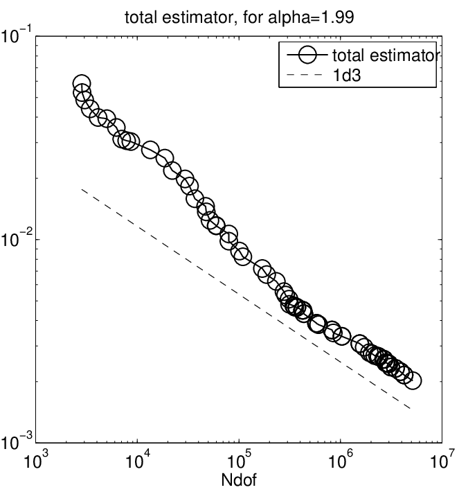
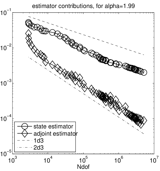
Refer to caption
Refer to caption
Figure 5. Example 4: The error estimator ℰ𝗈𝖼𝗉\mathscr{E}_{\mathsf{ocp}} and its contributions ℰ𝗒\mathscr{E}_{\mathsf{y}} and ℰ𝗉\mathscr{E}_{\mathsf{p}}.
Refer to caption
Refer to caption
Refer to caption
Refer to caption
Figure 6. Example 5: The error ‖(e𝗒¯,e𝗉¯,e𝗎¯)‖Ω\|(e_{\bar{\mathsf{y}}},e_{\bar{\mathsf{p}}},e_{\bar{\mathsf{u}}})\|_{\Omega} and error estimator ℰ𝗈𝖼𝗉\mathscr{E}_{\mathsf{ocp}}, their contributions ‖∇e𝗒¯‖L2​(ρ,Ω)\|\nabla e_{\bar{\mathsf{y}}}\|_{L^{2}(\rho,\Omega)}, ‖e𝗉¯‖L∞​(Ω)\|e_{\bar{\mathsf{p}}}\|_{L^{\infty}(\Omega)}, ‖e𝗎¯‖ℝl\|e_{\bar{\mathsf{u}}}\|_{\mathbb{R}^{l}}, ℰ𝗒\mathscr{E}_{\mathsf{y}} and ℰ𝗉\mathscr{E}_{\mathsf{p}}, and the effectivity index ℰ𝗈𝖼𝗉/‖(e𝗒¯,e𝗉¯,e𝗎¯)‖Ω\mathscr{E}_{\mathsf{ocp}}/\|(e_{\bar{\mathsf{y}}},e_{\bar{\mathsf{p}}},e_{\bar{\mathsf{u}}})\|_{\Omega}.
Refer to caption
Refer to caption
Figure 7. Example 6: The error estimator ℰ𝗈𝖼𝗉\mathscr{E}_{\mathsf{ocp}} and its contributions ℰ𝗒\mathscr{E}_{\mathsf{y}} and ℰ𝗉\mathscr{E}_{\mathsf{p}}.

References

  • [1] J.P. Agnelli, E.M. Garau, and P. Morin. A posteriori error estimates for elliptic problems with Dirac measure terms in weighted spaces. ESAIM Math. Model. Numer. Anal., 48(6):1557–1581, 2014.
  • [2] H. Aimar, M. Carena, R. Durán, and M. Toschi. Powers of distances to lower dimensional sets as Muckenhoupt weights. Acta Math. Hungar., 143(1):119–137, 2014.
  • [3] M. Ainsworth and J.T. Oden. A posteriori error estimation in finite element analysis. Pure and Applied Mathematics (New York). Wiley-Interscience, New York, 2000.
  • [4] A. Allendes, E. Otárola, R. Rankin, and A. J. Salgado. Adaptive finite element methods for an optimal control problem involving dirac measures. Numerische Mathematik, pages 1–39, 2017.
  • [5] P.R. Amestoy, I.S. Duff, and J.-Y. L’Excellent. Multifrontal parallel distributed symmetric and unsymmetric solvers. Comput. Methods in Appl. Mech. Eng., 184(2‚Äì4):501 – 520, 2000.
  • [6] P.R. Amestoy, I.S. Duff, J.-Y. L’Excellent, and J. Koster. A fully asynchronous multifrontal solver using distributed dynamic scheduling. SIAM J. Matrix Anal. Appl., 23(1):15–41 (electronic), 2001.
  • [7] H. Antil, E. Otárola, and A.J. Salgado. Some applications of weighted norm inequalities to the analysis of optimal control problems. IMA J. Numer. Anal., 2017.
  • [8] T. Apel, O. Benedix, D Sirch, and B. Vexler. A priori mesh grading for an elliptic problem with Dirac right-hand side. SIAM J. Numer. Anal., 49(3):992–1005, 2011.
  • [9] F. Camacho and A. Demlow. L2 and pointwise a posteriori error estimates for fem for elliptic pdes on surfaces. IMA J. Numer. Anal., 35(3):1199–1227, 2015.
  • [10] E. Casas. L2L^{2} estimates for the finite element method for the Dirichlet problem with singular data. Numer. Math., 47(4):627–632, 1985.
  • [11] C. D’Angelo. Finite element approximation of elliptic problems with Dirac measure terms in weighted spaces: applications to one- and three-dimensional coupled problems. SIAM J. Numer. Anal., 50(1):194–215, 2012.
  • [12] E. Dari, R.G. Durán, and C. Padra. Maximum norm error estimators for three-dimensional elliptic problems. SIAM J. Numer. Anal., 37(2):683–700, 2000.
  • [13] M. Dauge. Neumann and mixed problems on curvilinear polyhedra. Integral Equations Operator Theory, 15(2):227–261, 1992.
  • [14] A. Demlow and E.H. Georgoulis. Pointwise a posteriori error control for discontinuous Galerkin methods for elliptic problems. SIAM J. Numer. Anal., 50(5):2159–2181, 2012.
  • [15] A. Demlow and N. Kopteva. Maximum-norm a posteriori error estimates for singularly perturbed elliptic reaction-diffusion problems. Numer. Math., 133(4):707–742, 2016.
  • [16] J. Duoandikoetxea. Fourier analysis, volume 29 of Graduate Studies in Mathematics. American Mathematical Society, Providence, RI, 2001.
  • [17] K. Eriksson. An adaptive finite element method with efficient maximum norm error control for elliptic problems. Math. Models Methods Appl. Sci., 04(03):313–329, 1994.
  • [18] E.B. Fabes, C.E. Kenig, and R.P. Serapioni. The local regularity of solutions of degenerate elliptic equations. Comm. Part. Diff. Eqs., 7(1):77–116, 1982.
  • [19] D. Gilbarg and N. S. Trudinger. Elliptic partial differential equations of second order. Classics in Mathematics. Springer-Verlag, Berlin, 2001. Reprint of the 1998 edition.
  • [20] V. Gol′dshtein and A. Ukhlov. Weighted Sobolev spaces and embedding theorems. Trans. Amer. Math. Soc., 361(7):3829–3850, 2009.
  • [21] W. Gong, G. Wang, and N. Yan. Approximations of elliptic optimal control problems with controls acting on a lower dimensional manifold. SIAM J. Control Optim., 52(3):2008–2035, 2014.
  • [22] L. Grafakos. Modern Fourier analysis, volume 250 of Graduate Texts in Mathematics. Springer, New York, third edition, 2014.
  • [23] P. Grisvard. Elliptic problems in nonsmooth domains, volume 69 of Classics in Applied Mathematics. Society for Industrial and Applied Mathematics (SIAM), Philadelphia, PA, 2011. Reprint of the 1985 original [ MR0775683], With a foreword by Susanne C. Brenner.
  • [24] M. Grüter and K.-O. Widman. The Green function for uniformly elliptic equations. Manuscripta Math., 37(3):303–342, 1982.
  • [25] M. Hintermüller, R.H.W. Hoppe, Y. Iliash, and M. Kieweg. An a posteriori error analysis of adaptive finite element methods for distributed elliptic control problems with control constraints. ESAIM: Control Optim. Calc. of Var., 14:540–560, 7 2008.
  • [26] S. Hofmann and S. Kim. The Green function estimates for strongly elliptic systems of second order. Manuscripta Math., 124(2):139–172, 2007.
  • [27] D. Jerison and C.E. Kenig. The inhomogeneous Dirichlet problem in Lipschitz domains. J. Funct. Anal., 130(1):161–219, 1995.
  • [28] D. S. Jerison and C. E. Kenig. The Neumann problem on Lipschitz domains. Bull. Amer. Math. Soc. (N.S.), 4(2):203–207, 1981.
  • [29] J. Jost. Partial differential equations, volume 214 of Graduate Texts in Mathematics. Springer, New York, third edition, 2013.
  • [30] K. Kohls, A. Rösch, and K.G. Siebert. A posteriori error analysis of optimal control problems with control constraints. SIAM J. Control Optim., 52(3):1832–1861, 2014.
  • [31] T. Köppl and B. Wohlmuth. Optimal a priori error estimates for an elliptic problem with Dirac right-hand side. SIAM J. Numer. Anal., 52(4):1753–1769, 2014.
  • [32] V.A Kozlov, V.G Maz’ya, and J. Rossmann. Elliptic boundary value problems in domains with point singularities. American Mathematical Society, Providence, Rhode Island, USA, 1997.
  • [33] J.-L. Lions. Optimal control of systems governed by partial differential equations. Translated from the French by S. K. Mitter. Die Grundlehren der mathematischen Wissenschaften, Band 170. Springer-Verlag, New York-Berlin, 1971.
  • [34] W. Liu and N. Yan. A posteriori error estimates for distributed convex optimal control problems. Adv. in Comput. Math., 15(1-4):285–309, 2001.
  • [35] V. Maz’ya and J. Rossmann. Elliptic equations in polyhedral domains, volume 162 of Mathematical Surveys and Monographs. American Mathematical Society, Providence, RI, 2010.
  • [36] D. Mitrea and I. Mitrea. On the regularity of Green functions in Lipschitz domains. Comm. Partial Differential Equations, 36(2):304–327, 2011.
  • [37] P. Morin, R. H. Nochetto, and K. G. Siebert. Data oscillation and convergence of adaptive FEM. SIAM J. Numer. Anal., 38(2):466–488 (electronic), 2000.
  • [38] B. Muckenhoupt. Weighted norm inequalities for the Hardy maximal function. Trans. Amer. Math. Soc., 165:207–226, 1972.
  • [39] R.H. Nochetto. Pointwise a posteriori error estimates for elliptic problems on highly graded meshes. Math. Comp., 64(209):1–22, 1995.
  • [40] R.H. Nochetto, E. Otárola, and A.J. Salgado. Piecewise polynomial interpolation in Muckenhoupt weighted Sobolev spaces and applications. Numer. Math., 132(1):85–130, 2016.
  • [41] R.H. Nochetto, A. Schmidt, K.G. Siebert, and A. Veeser. Pointwise a posteriori error estimates for monotone semi-linear equations. Numer. Math., 104(4):515–538, 2006.
  • [42] R.H. Nochetto, G.K. Siebert, and A. Veeser. Pointwise a posteriori error control for elliptic obstacle problems. Numer. Math., 95(1):163–195, 2002.
  • [43] R.H. Nochetto, K.G. Siebert, and A. Veeser. Theory of adaptive finite element methods: an introduction. In Multiscale, nonlinear and adaptive approximation. Springer, 2009.
  • [44] R.H. Nochetto and A. Vesser. Primer of adaptive finite element methods. In Multiscale and Adaptivity: Modeling, Numerics and Applications, CIME Lectures. Springer, 2011.
  • [45] G. Savaré. Regularity results for elliptic equations in Lipschitz domains. J. Funct. Anal., 152(1):176–201, 1998.
  • [46] R. Schneider and G. Wachsmuth. A Posteriori Error Estimation for Control-Constrained, Linear-Quadratic Optimal Control Problems. SIAM J. Numer. Anal., 54(2):1169–1192, 2016.
  • [47] L.R. Scott. Finite element convergence for singular data. Numer. Math., 21:317–327, 1973/74.
  • [48] L.R. Scott and S. Zhang. Finite element interpolation of nonsmooth functions satisfying boundary conditions. Math. Comp., 54(190):483–493, 1990.
  • [49] F. Tröltzsch. Optimal control of partial differential equations, volume 112 of Graduate Studies in Mathematics. American Mathematical Society, Providence, RI, 2010. Theory, methods and applications, Translated from the 2005 German original by Jürgen Sprekels.
  • [50] B.O. Turesson. Nonlinear potential theory and weighted Sobolev spaces. Springer, 2000.
  • [51] R. Verfürth. A posteriori error estimators for the Stokes equations. Numer. Math., 55(3):309–325, 1989.
  • [52] R. Verfürth. A posteriori error estimation techniques for finite element methods. Numerical Mathematics and Scientific Computation. Oxford University Press, Oxford, 2013.