Cheillini integrability and quadratically damped oscillators
Abstract
In this paper a new approach to study an equation of the Liénard type with a strong quadratic damping is proposed based on Jacobi’s last multiplier and Cheillini’s integrability condition. We obtain a closed form solution of the transcedental characteristic equation of the Liénard type equation using the Lambert -function.
Mathematics Classification (2010)
:34C15, 34C20.
Keywords:
Quadratic damping. Liénard equation, Cheillini integrability condition, Lambert function.
1 Introduction
In recent times a number of articles have appeared in the literature which deal with the phenomenon of a linear oscillator subject to a quadratic damping force [3, 4, 5, 10, 11]. Most elementary textbooks deal with viscous damping for the obvious reason that it involves a linear dependance on the velocity of the oscillator and presents the simplest situation where an exact analytical treatment is possible. In general this involves analysis of a second-order ordinary differential equation (ODE) of the Liénard type [13], namely , where it is assumed that is a constant and the function . As damping does not arise from a single physical phenomena and is itself of various kinds, e.g., material damping, structural damping, interfacial damping, aerodynamic and hydrological drag etc., therefore a different mathematical description is needed in each case. Systems like the simple harmonic oscillator and the viscously damped harmonic oscillator, both of which can be solved by standard undergraduate mathematical techniques, however, represent idealizations of real life phenomena because they ignore nonlinear aspects of the forcing term as well as the damping force. A more realistic model in which damping is proportional to the square of the velocity is usually common at higher velocities and is applicable to problems involving hydrological drag and in aerodynamics. When an immersed object moves through a fluid at relatively high Reynolds numbers [14]- the corresponding drag force is found to be proportional to the square of the velocity . Oscillators with a non-negative real-power restoring force and quadratic damping have been recently studied by Kovacic and Rakaric [11].
The principal feature associated with quadratic damping is a discontinuous jump of the damping force in the
equation of motion whenever the velocity vanishes such that the frictional force always opposes the motion.
In case of oscillatory systems this occurs every half cycles and means that instead of a single equation of
motion the latter splits into two parts depending on the sign of the velocity. Each equation has to solved
separately and matched at the points where the velocity changes sign. In general solving such a system in
presence of nonlinearity proves to be a rather daunting task and only in rare cases is an exact solution
to be expected. Numerical techniques on the other hand provide valuable information about the
evolution of the system and its general nature.
From the mathematical point of view the construction of first integrals for systems involving a quadratic
dependance on the velocity often provides interesting insights. Indeed constants of motion are the bed
rock of many of the conservation principles at the heart of theoretical physics: the work-energy
theorem applied to a conservative system, is perhaps the most striking and oft quoted example,
as it has evolved into the principle of conservation of energy.
In this paper we examine the equation , ,
in the light of several recent articles which have also dealt
with the same equation. This is a discontinuous generalization of an equation of the Liénard type
involving a quadratic dependence on the velocity. The issue of isochronicity
in such equations was extensively studied in [18, 6, 8].
In particular we show that by imposing the Cheillini condition of integrability on the
functions and one can subsume many of the previous examples into a compact scheme.
Incidentally the Cheillini condition is typically encountered in the context of
integrability of the standard Liénard equation in course of its transformation to the
first-order Abel equation of the first kind and also while finding a Lagrangian/Hamiltonian
description of the Liénard equation [9]. However, its application to the case of quadratic
damping appears to be new. We show how one can derive in a systematic manner the maximum
amplitudes analytically in terms of the Lambert function.
The organization of the paper is as follows. In Section 2 we review a second-order ODE with a quadratic dependence on velocity in the context of its Lagrangian/Hamiltonian description. It is shown that such a system may be interpreted as one displaying a position dependent mass function. The trajectory is explicitly displayed by numerical investigations. In Section 3 we split the ODE into two parts as mentioned above depending on the sign of the velocity and investigate the trajectories, maximum amplitudes as well as period of oscillations. In particular we show that the periods of the cycles and the corresponding maximum amplitudes are both determined exclusively by a potential function which involves the position dependent mass function. Furthermore by invoking the Cheillini integrability condition it is possible to write down analytic formulae for the maximum amplitudes in terms of the Lambert function [2], named after the eighteenth century scientist J. H. Lambert [12]. The Lambert function is defined as the inverse function of the mapping and thus solves the equation. equation. This solution is given in the form of the Lambert function, , i.e. satisfies . This equation always has an infinite number of solutions, most of which are complex, and is a multivalued function. The examples presented here also includes those obtained earlier by Cveticanin [3, 4].
2 The Hamiltonian in presence of quadratic velocity
Consider a second-order ODE with a quadratic dependance on the velocity given by
| (2.1) |
we assume and are such that and is integrable while . The functional form of where is analytic. As demonstrated in [15, 16], the Jacobi Last Multiplier (JLM) provides a convenient tool for obtaining a Lagrangian for second-order equations of the form . It is defined as a solution of
| (2.2) |
In the present case it follows that
| (2.3) |
The relationship between the JLM, and the Lagrangian is provided by as a consequence of which for (2.1) the Lagrangian may be expressed in the form
| (2.4) |
where is determined by substituting (2.4) into the Euler-Lagrange equation
which immediately gives
| (2.5) |
By means of the standard Legendre transformation we can obtain the Hamiltonian as
| (2.6) |
It is easily verified that the Hamiltonian is a constant of motion and the expression for the conjugate momentum suggests that serves as a position dependent mass term. In fact equations with quadratic velocity dependance of the type considered here naturally arise in the Newtonian formulation of the equation of motion of a particle with a variable mass. Clearly then, the trajectories for arbitrary intial condition where are given by
| (2.7) |
In terms of the canonical momentum, , the Hamiltonian becomes
| (2.8) |
Defining a new set of canonical variables
| (2.9) |
the Hamiltonian takes the appearance
| (2.10) |
and corresponds to that of a particle of unit mass provided is invertible. In the following we consider a simple example in which and . Let , so that . Then momentum and coordinate becomes and respectively, and . Thus in terms of new coordinates the Hamiltonian has the following form
| (2.11) |

3 Quadratic damping
It is plain that (2.1) can not describe a system with a quadratic damping as the term involving does not change sign and oppose the motion when the velocity reverses its sign. To remedy this feature it is necessary to split (2.1) into two parts and write
| (3.1) |
| (3.2) |
Let us denote the Hamiltonians associated with the pieces by
| (3.3) |
with the superscript standing for . Furthermore it will be assumed that the initial point with to be such that and . Thus when motion commences from the initial point then the trajectory is defined by or in explicit form
This trajectory crosses the -axis first at say when the velocity . Consequently the point of intersection which denotes the maximum amplitude is determined from the equation , i.e., from
| (3.4) |
Continuing the trajectory to below the -axis means that it is now determined by the equation
where the constant is determined by the new initial condition which represents the first turning point. This gives so that beneath the -axis the trajectory is given by
At the next turning point we have and
| (3.5) |
whcih allows for the determination of . After this we are again above the -axis and the trajectory is given by with . Continuing in this manner we may summarise the points of intersections with the -axis by stating that:
if odd then is determined by
and if even then is determined by
3.1 Closed and Damped Orbits
Systems given by (3.1) and (3.2) do not always show damped behaviour. The qualitative features of such systems depends on . To study such systems, we consider two cases: with ,
respectively. Figure [2] shows the plot for both the cases in phase
space. When the amplitude continuously diminishes and the trajectory is a spiral. Table 1 below
gives the values of the amplitudes for each half of the cycle. In this case the dampening force has the same sign in each of the four quadrants as the linear damped oscillator.
| Amplitudes () | ||||
|---|---|---|---|---|
| 0.7680390470134656 | ||||
| 0.5049710640693359 | ||||
| 0.37698121404812546 | ||||
| 0.3009607508865283 | ||||
| 0.2505262046138416 | ||||
| 0.21459868739856763 | ||||
| 0.18769746691321143 | ||||
| 0.166796834446442 | ||||
| 0.15008870326261628 |
However when one finds that the orbits are closed. Figure [2] shows the orbits for four initial conditions. In this case the dampening force alternates in sign in each of the four quadrants.


In our case, the potentials are denoted by . Figure [3] shows the potential plots for both the cases under study. From the figure, it is clear that there are initial conditions for which bounded solutions exists in both the cases.


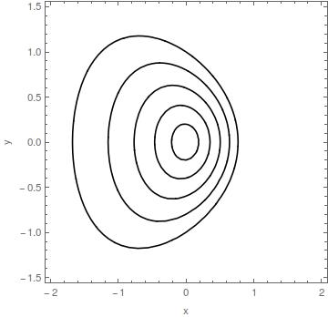
Now, consider the kinetic part. In our case the mass term is position dependent and plays the key role in whether there is closed or damp orbit. The main idea is the mass term depends on only. Consider figure [4] of contour plots of Hamiltonian in the two cases. In the first case, is constant and so even and therefore is odd. While in the second case, is odd function and is even and its evident from the plots that Hamiltonian is symmetric about the .


Figure [5] depicts the behaviour of higher degree functions.


3.2 Analytic results based on Cheillini integrability condition
It is interesting to observe that invocation of the Cheillini condition for integrability allows us to determine analytically the maximum amplitudes. This may be accomplished by noting that as
so integrating by parts we obtain
where the Cheillini integrability condition
| (3.6) |
has been used. From this condition we have where is an arbitrary constant of integration. Of course, if and are given beforehand then the values of the constants and can be simply read off from the above ratio assuming the Cheillini condition to hold. By defining and the function the last expression for the potential can be put into the form
| (3.7) |
As mentioned in (2.4) the first turning point is given by a solution of which is positive or more explicitly by a positive solution of
| (3.8) |
In general it is possible to find recursively the subsequent turning points which are the solutions with proper signs of the equation
| (3.9) |
Eqn.(3.9) has the appearance which is the the standard form of the Lambert equation and its solutions are given by the Lambert function, i.e, . Hence it follows that
| (3.10) |
from which we can determine formally
| (3.11) |
if the function is invertible. We therefore conclude that if the Cheillini condition is fulfilled by the functions and then the maximum amplitudes can be determined recursively in terms of the Lambert function.
3.3 Analysis of the period function
Starting from the initial point if the first intersection with the -axis is at then subsequently the trajectory is determined by the condition
If the next turning point, i.e., the next intersection with the negative -axis is at then the time for the transit of the half-cycle from to is given by
| (3.12) |
Similarly the time taken for the transit of the next-half cycle from on the negative -axis to on the positive -axis is given by
| (3.13) |
Thus the time taken for the completion of the first cycle is , viz
| (3.14) |
In fact it is straightforward to generalize this formula for the -th cycle which is given by
| (3.15) |
The energy dissipated in the -th cycle is given by
| (3.16) |
Table 2 gives the values of time periods and change in energy for the case and Table 3 gives the time periods for the closed orbits in the case for different initial conditions. In our case we have assumed that the energy is given by the Hamiltonian and differs from the expression used in [3].
| Cycle() | |||
|---|---|---|---|
| 6.360502498547287 | 0.08805266518005395 | ||
| 6.308066845017076 | 0.01833863366586541 | ||
| 6.295534499523865 | 0.006618943128696708 | ||
| 6.29057350609154 | 0.0031022724220284292 | ||
| 6.288104015677968 | 0.0016959179654737477 | ||
| 6.286695917618085 | 0.0010263408918240735 | ||
| 6.285816631877343 | 0.0006676772782294726 | ||
| 6.285230961390923 | 0.0004584700142998832 | ||
| 6.284821348882355 | 0.0003283012470082225 |
| i=() | ||
|---|---|---|
| 6.197928744154146 | ||
| 6.111126244536706 | ||
| 6.014565567199962 | ||
| 5.918345639978987 |
4 Conclusion
In this paper, a Liénard type equation with quadratic damping has been considered. We have shown that by imposing the Cheillini condition of integrability on the functions and one can demonstrate many of the previous examples into a compact scheme. Incidentally the Cheillini condition is typically encountered in the context of integrability of the standard Liénard equation in course of its transformation to the first-order Abel equation of the first kind and also while finding a Lagrangian/Hamiltonian description of the Liénard equation. Our next target is to study generalized oscillatory equation with a non-negative real-power restoring force and quadratic damping and seek for the solution and other dynamical features of this type of equations. In particular, we wish to generalize Kovacic et al. [11] model where they have considered purely non-linear restoring force of the type ,
Acknowledgement
The authors are grateful to Professor Livija Cveticanin for various useful discussions They are also thankful to Professor Asok Mallik for his interest and encouragement and one of us (PG) wishes to acknowledge “Dynamics of Complex Systems, DCS-2016” programme at ICTS-TIFR for their gracious hospitality where part of the work has been done.
References
- [1] A. Chiellini, Sull’integrazione dell’equazione differenziale , Bollettino dell’Unione Matematica Italiana, 10, 301-307 (1931).
- [2] R.M. Corless, G. H. Gonnet, D. E. G. Hare, D. J. Jeffrey, and D. E. Knuth, On the Lambert W function. Advances Computational Maths 5 (1996), 329-359.
- [3] L. Cveticanin, Oscillator with strong quadratic damping force, Publ. Inst. Math. (Beograd) (N.S.) 85(99) (2009), 119–130.
- [4] L. Cveticanin, Analysis techniques for the various forms of the Duffing equation in The Duffing Equation: Nonlinear Oscillators and their Behaviour, 81–137, Ed. I. Kovacic and M. J. Brennan, Wiley, Chichester, 2011.
- [5] T. H. Fay, Quadratic damping. Internat. J. Math. Ed. Sci. Tech. 43 (2012), no. 6, 789-803.
- [6] A. Ghose Choudhury and P. Guha, On isochronous cases of the Cherkas system and Jacobi’s last multiplier, J. Phys. A: Math. Theor. 43 (2010) 125202.
- [7] A. Ghose Choudhury and P. Guha, An analytic technique for the solutions of nonlinear oscillators with damping using the Abel Equation, to appear in Discontinuity, Nonlinearity and Complexity.
- [8] P. Guha and A. Ghose Choudhury, The Jacobi last multiplier and isochronicity of Liénard type systems, Rev. Math. Phys. 25 (6) (2013) 1330009.
- [9] T. Harko, F. S. N. Lobo, M. K. Mak, A Chiellini type integrability condition for the generalized first kind Abel differential equation, Universal Journal of Applied Mathematics, 1 (2013 101-104.
- [10] K. Klotter, Free oscillations of systems having quadratic damping and arbitrary restoring forces. J. Appl. Mech. 22 (1955), 493-499.
- [11] I. Kovacic and Z. Rakaric, Study of oscillators with a non-negative real-power restoring force and quadratic damping. Nonlinear Dynam. 64 (2011), no. 3, 293-304.
- [12] J.H.Lambert,Acta Helvitica 3 (1758) 128-168.
- [13] A. Liénard, Revue générale de l’électricité 23, 901- 912, and 946-954 (1928).
- [14] A. H. Nayfeh and D. Mook, Nonlinear Oscillations, Wiley, New York, 1979.
- [15] M.C.Nucci and P.G.L.Leach, The Jacobi’s Last Multiplier and its applications in mechanics, J. Phys. Scr. 78(2008) 065011.
- [16] M.C. Nucci and K.M. Tamizhmani, Lagrangians for dissipative nonlinear oscillators: the method of Jacobi last multiplier, Journal of Nonlinear Mathematical Physics, Vol. 17, No. 2 (2010) 167178.
- [17] A. D. Polyanin and V. F. Zaitsev, Handbook of Exact Solutions for Ordinary Differential Equations, Chapman & Hall/CRC, Boca Raton, London, New York, Washington, D. C. (2003).
- [18] M Sabatini, On the period Function of Liénard Systems, J. Diff. Eqns. 152,467-487, (1999).