Highly polarized components of integrated pulse profiles
Abstract
Highly polarized components of pulse profiles are investigated by analyzing observational data and simulating the emission processes. The highly polarized components appear at the leading or trailing part of a pulse profile, which preferably have a flat spectrum and a flat polarization angle curve compared with the low polarized components. By considering the emission processes and propagation effects, we simulate the distributions of wave modes and fractional linear polarization within the entire pulsar emission beam. We show that the highly polarized components can appear at the leading, central, and/or trailing parts of pulse profiles in the models, depending on pulsar geometry. The depolarization is caused by orthogonal modes or scattering. When a sight line cuts across pulsar emission beam with a small impact angle, the detected highly polarized component will be of the O mode, and have a flat polarization angle curve and/or a flat spectrum as observed. Otherwise, the highly polarized component will be of the X mode and have a steep polarization angle curve.
Keywords:
pulsars: general – polarization – acceleration of particles1 INTRODUCTION
Integrated pulse profiles are obtained by integrating tens of thousands of individual pulses. Features of pulse profiles have been investigated to understand the geometry and physical processes within pulsar magnetosphere (Rankin, 1983; Lyne & Manchester, 1988; Kramer et al., 1994; Noutsos et al., 2015, e.g.). Integrated pulse profiles generally comprise several components, and are characterized by diverse polarization features, including prominent linear polarization, ‘S’-shaped polarization angle curves, single sign or sign reversals of circular polarization. Some integrated pulse profiles are highly polarized for the whole pulse, even 100% polarized such as PSR B1259-63 and B1823-13. These pulsars are generally young and have very high spin-down luminosity and flat spectrum (Qiao et al., 1995; von Hoensbroech et al., 1998; Crawford et al., 2001; Weltevrede & Johnston, 2008). Some pulsars have highly linearly polarized leading or trailing components, for example, the leading components of PSRs B0355+54 and B0450+55 (Lyne & Manchester, 1988; von Hoensbroech & Xilouris, 1997; Gould & Lyne, 1998), and the trailing components of PSRs B1650-38 and B1931+24 (Karastergiou et al., 2005; Han et al., 2009). von Hoensbroech et al. (1998) noticed that the highly polarized leading component of PSR B0355+54 has a flat spectrum and becomes increasingly prominent at higher frequencies. The highly polarized trailing component of PSR B2224+65 has a flat polarization angle curve (Mitra & Rankin, 2011).
 |
 |
Theoretical efforts have been made to understand various polarization features. In general, pulsar polarizations are closely related to the emission processes of the relativistic particles streaming along the curved magnetic field lines (Blaskiewicz et al., 1991; Wang et al., 2012, e.g.), the propagation effects within pulsar magnetosphere (Barnard & Arons, 1986; Wang et al., 2010; Beskin & Philippov, 2012, e.g.), and the scattering within the interstellar medium (Li & Han, 2003). However, these investigations have been conducted separately on each aspect, rarely done jointly. Curvature radiation which serves as one of the most probable mechanisms for pulsar emission can produce highly polarized emission (Gangadhara, 2010; Wang et al., 2012). Propagation effects are succeeded in demonstrating the interaction of the ordinary (O) and extra-ordinary (X) modes within pulsar magnetosphere and can lead to diverse depolarization features (Cheng & Ruderman, 1979; Barnard & Arons, 1986; Wang et al., 2010; Beskin & Philippov, 2012), though initial ratios for both modes are uncertain. Propagation effects within the interstellar medium need to be investigated further. Recently, we investigated the emission processes jointly with propagation effects (Wang et al., 2014; Wang et al., 2015), which provides us a new opportunity to understand the highly polarized components, because distributions of the X-mode and O-mode within pulsar magnetosphere are related to the depolarization across pulsar emission beam by considering the refraction and corotation effects. Emission can be highly depolarized in some beam regions where both modes have comparable intensities, but dominated by one mode in other regions and hence the resulting profile can be highly polarized.
In this paper, we summarize observations for highly polarized components of integrated pulse profiles in literature and then theoretically explain them by modeling emission and propagation processes. In Section 2, we analyze various features for highly polarized components of observed pulsar profiles. In Section 3, we simulate polarized pulsar beams and pulse profiles by considering the emission processes and propagation effects. Discussions and conclusions are given in Section 4.
| PSR Jname | Bname | Period | DM | Polarization Features | References |
| (s) | () | ||||
| J0014+4746 | B0011+47 | 1.24069 | 30.8 | Leading | 31, 70, 86 |
| J0358+5413 | B0355+54 | 0.15638 | 57.1 | Leading, Flat Spec., Orth. Modes | 8, 9, 16, 20, 24, 26, 30, 31, 34, 77, 81 |
| J0454+5543 | B0450+55 | 0.34072 | 14.5 | Leading, Flat Spec., Flat PA | 16, 20, 30, 31, 81 |
| J0814+7429 | B0809+74 | 1.29224 | 5.7 | Leading, Orth. Modes | 1, 9, 30, 31, 44, 58, 78, 88 |
| J0942-5657 | B0941-56 | 0.80812 | 159.7 | Leading | 23, 33, 69, 90 |
| J0954-5430 | 0.47283 | 200.3 | Leading | 69, 90 | |
| J1048-5832 | B1046-58 | 0.12367 | 129.1 | Leading, Flat Spec. | 23, 56, 59, 69, 76, 89, 90 |
| J1057-5226IP | B1055-52 | 0.19710 | 30.1 | Leading, Flat Spec. | 4, 6, 12, 16, 29, 69, 72, 77, 89, 90 |
| J1112-6103 | 0.06496 | 599.1 | Leading, Scattering | 69, 89, 90 | |
| J1341-6220 | B1338-62 | 0.19333 | 717.3 | Leading, Scattering | 23, 39, 59, 60, 69, 90 |
| J1410-6132 | 0.05005 | 960.0 | Leading, Scattering | 68, 69, 89, 90 | |
| J1453-6413 | B1449-64 | 0.17948 | 71.0 | Leading, Flat PA, Orth. Modes | 5, 6, 7, 29, 54, 59, 69, 71, 81, 90 |
| J1730-3350 | B1727-33 | 0.13946 | 259.0 | Leading, Scattering | 31, 39, 59, 69, 89, 90 |
| J1805+0306 | B1802+03 | 0.21871 | 80.8 | Leading, Flat PA | 31, 38 |
| J1823-3106 | B1820-31 | 0.28405 | 50.2 | Leading | 21, 31 |
| J1825-0935MP | B1822-09 | 0.76900 | 19.3 | Leading, Flat Spec., Orth. Modes | 7, 9, 24, 29, 30, 31, 49, 61, 63, 65, 73, 77 |
| J1844+1454 | B1842+14 | 0.37546 | 41.4 | Leading, Flat Spec., Flat PA | 17, 31, 38, 54, 65, 74, 77, 81, 90 |
| J1849+2423 | 0.27564 | 62.2 | Leading | 70 | |
| J1937+2544 | B1935+25 | 0.20098 | 53.2 | Leading, Flat PA | 31, 38, 63, 70, 81, 90 |
| J2008+2513 | 0.58919 | 60.5 | Leading, Orth. Modes | 70 | |
| J0601-0527 | B0559-05 | 0.39596 | 80.5 | Trailing, Flat Spec., Flat PA | 20, 23, 31, 34, 54, 69, 90 |
| J0922+0638 | B0919+06 | 0.43062 | 27.2 | Trailing, Flat Spec., Orth. Modes | 13, 19, 24, 29–31, 38, 49, 54, 59 |
| 62, 65, 74, 81, 90 | |||||
| J1401-6357 | B1358-63 | 0.84278 | 98.0 | Trailing | 21, 23, 29 |
| J1539-5626 | B1535-56 | 0.24339 | 175.8 | Trailing, Flat Spec., Flat PA | 23, 56, 59, 69, 90 |
| J1548-5607 | 0.17093 | 315.5 | Trailing | 69, 90 | |
| J1653-3838 | B1650-38 | 0.30503 | 207.2 | Trailing | 56, 69, 90 |
| J1739-1313 | 1.21569 | 58.2 | Trailing | 69, 90 | |
| J1808-3249 | 0.36491 | 147.3 | Trailing | 56, 69, 90 | |
| J1933+2421 | B1931+24 | 0.81369 | 106.0 | Trailing | 31, 70 |
| J2013+3845 | B2011+38 | 0.23019 | 238.2 | Trailing, Flat PA | 31, 81 |
| J2225+6535 | B2224+65 | 0.68254 | 36.0 | Trailing, Flat Spec., Flat PA | 9, 16, 31, 77, 86, 88 |
| J0737-3039A | 0.02269 | 48.9 | MSP, Leading&Trailing | 47, 55, 57, 82 | |
| Flat PA, Orth. Mod | |||||
| J1012+5307 | 0.00525 | 9.0 | MSP, Trailing, Flat PA | 35, 37, 70, 88 | |
| J1022+1001 | 0.01645 | 10.2 | MSP, Trailing | 35–37, 46, 48, 52, 80, 84, 85, 87, 88 | |
| J1300+1240 | B1257+12 | 0.00621 | 10.1 | MSP, Leading | 35, 70 |
| J0108-1431 | 0.80756 | 2.3 | Whole | 33, 69, 90 | |
| J0134-2937 | 0.13696 | 21.8 | Whole | 33, 65, 69, 71, 90 | |
| J0139+5814 | B0136+57 | 0.27245 | 73.7 | Whole | 16, 20, 30, 31, 81, 86, 88 |
| J0538+2817 | 0.14315 | 39.5 | Whole | 30, 81 | |
| J0543+2329 | B0540+23 | 0.24597 | 77.7 | Whole, Pol. dec. with freq. | 9, 10, 17, 19, 24, 30, 31, 38, 49 |
| 53, 63, 65, 69, 74, 77, 81, 90 | |||||
| J0614+2229 | B0611+22 | 0.33495 | 96.9 | Whole, Strong CP | 10, 16, 19, 31, 34, 38, 53, 63, 65, 69, 74 |
| J0630-2834 | B0628-28 | 1.24441 | 34.4 | Whole | 5, 6, 7, 9, 16, 29, 31, 34, 54, 59, 65, 69, 81, 90 |
| J0631+1036 | 0.28780 | 125.3 | Whole | 27, 69, 75, 89, 90 | |
| J0659+1414 | B0656+14 | 0.38489 | 13.9 | Whole | 17, 31, 38, 40, 53, 59, 63, 64, 69, 74 |
| 75, 81, 89, 90 | |||||
| J0742-2822 | B0740-28 | 0.16676 | 73.7 | Whole | 6, 7, 9, 16, 24, 29–31, 33, 49, 54, 59 |
| 61, 69, 71, 75, 77, 81, 83, 89, 90 | |||||
| J0835-4510 | B0833-45 | 0.08932 | 67.9 | Whole, Strong CP | 2, 3, 5–7, 11, 29, 43, 54, 59, 61 |
| 69, 71, 76, 81, 89, 90 | |||||
| J0901-4624 | 0.44199 | 198.8 | Whole, Strong CP | 69, 90 | |
| J0905-5127 | 0.34628 | 196.4 | Whole | 69, 90 | |
| J0908-4913 | B0906-49 | 0.10675 | 180.3 | Whole, Inter Pulse | 21, 23, 32, 59, 66, 69, 76, 89, 90 |
| J1015-5719 | 0.13988 | 278.7 | Whole | 60, 69, 90 | |
| J1028-5819 | 0.09140 | 96.5 | Whole | 67, 69, 89 | |
| J1057-5226MP | B1055-52 | 0.19710 | 30.1 | Whole | 4, 6, 12, 16, 29, 69, 72,77, 89, 90 |
| J1105-6107 | 0.06319 | 271.0 | Whole | 39, 60, 69, 89, 90 |
| J1119-6127 | 0.40796 | 707.4 | Whole | 45, 60, 69, 79, 89, 90 | |
| J1302-6350 | B1259-63 | 0.04776 | 146.7 | Whole, Strong CP | 22, 25, 42, 56, 59, 69, 90 |
| J1321+8323 | B1322+83 | 0.67003 | 13.3 | Whole | 31, 70, 86 |
| J1359-6038 | B1356-60 | 0.12750 | 293.7 | Whole, Strong CP | 21, 29, 33, 59, 61, 69, 90 |
| J1420-6048 | 0.06817 | 358.8 | Whole, Strong CP | 41, 60, 69, 75, 89, 90 | |
| J1614-5048 | B1610-50 | 0.23169 | 582.8 | Whole, Scattering, Strong CP | 23, 56, 69, 90 |
| J1637-4553 | B1634-45 | 0.11877 | 193.2 | Whole | 56, 69, 90 |
| J1702-4128 | 0.18213 | 367.1 | Whole | 69, 89, 90 | |
| J1705-1906IP | B1702-19 | 0.29898 | 22.9 | Whole, Strong CP, Inter-pulse | 15, 16, 29, 31, 34, 49, 65, 69, 90 |
| J1705-3950 | 0.31894 | 207.1 | Whole, Strong CP | 69, 90 | |
| J1709-4429 | B1706-44 | 0.10245 | 75.6 | Whole, Strong CP | 23, 54, 56, 59, 69, 89, 90 |
| J1718-3825 | 0.07466 | 247.4 | Whole | 69, 75, 89, 90 | |
| J1733-3716 | B1730-37 | 0.33758 | 153.5 | Whole | 56, 69, 90 |
| J1740-3015 | B1737-30 | 0.60688 | 152.1 | Whole, Strong CP | 21, 23, 31, 34, 59, 69, 76, 90 |
| J1801-2451 | B1757-24 | 0.12491 | 289.0 | Whole, Strong CP | 31, 63, 69, 81, 86, 89, 90 |
| J1803-2137 | B1800-21 | 0.13366 | 233.9 | Whole, Strong CP | 21, 31, 34, 69, 86, 90 |
| J1809-1917 | 0.08274 | 197.1 | Whole, Strong CP | 69, 90 | |
| J1826-1334 | B1823-13 | 0.10148 | 231.0 | Whole, Strong CP | 31, 34, 69, 90 |
| J1830-1059 | B1828-11 | 0.40504 | 161.5 | Whole, Strong CP | 31, 69, 90 |
| J1841-0345 | 0.20406 | 194.3 | Whole | 69, 90 | |
| J1841-0425 | B1838-04 | 0.18614 | 325.4 | Whole | 31, 63, 69, 90 |
| J1850+1335 | B1848+13 | 0.34558 | 60.1 | Whole | 31, 38, 63, 65, 81, 90 |
| J1915+1009 | B1913+10 | 0.40454 | 241.6 | Whole, Strong CP | 17, 31, 34, 38, 63, 81, 90 |
| J1926+1648 | B1924+16 | 0.57982 | 176.8 | Whole | 10, 17, 19, 31, 38, 77 |
| J1932+1059 | B1929+10 | 0.22651 | 3.1 | Whole | 2, 9, 10, 13, 14, 16–20, 24, 26, 28–31, 37, 38 |
| 40, 49–51, 53, 54, 70, 74, 81, 86, 88, 90 |
Notes. Leading: Highly polarized (larger than 70%) leading components; Trailing: highly polarized trailing components; MSP: millisecond pulsars with highly polarized leading and/or trailing components; Whole: highly polarized for the whole pulse profiles; Flat Spec.: flat spectrum; Flat PA: flat polarization angle curves; Orth. Modes: orthogonal modes; Strong CP: strong circular polarization. References: (1) Lyne et al. (1971) at 0.151, 0.24, 0.408 GHz; (2) Manchester (1971) at 0.392, 1.665 GHz; (3) Komesaroff et al. (1974) at 4.83 GHz; (4) McCulloch et al. (1976) at 1.4 GHz; (5) Hamilton et al. (1977) at 0.338, 0.4 GHz; (6) McCulloch et al. (1978) at 0.631, 0.649 GHz; (7) Manchester et al. (1980) at 1.612 GHz; (8) Morris et al. (1980) at 2.65 GHz; (9) Morris et al. (1981) at 1.72, 2.65, 4.85, 8.7 GHz; (10) Rankin & Benson (1981) at 0.43 GHz; (11) Krishnamohan & Downs (1983) at 2.295 GHz; (12) Rankin (1983) at 0.17, 0.631 GHz; (13) Stinebring et al. (1984a) at 1.404 GHz; (14) Stinebring et al. (1984b) at 0.8 GHz; (15) Biggs et al. (1988) at 0.408 GHz; (16) Lyne & Manchester (1988) at 0.408, 0.415, 0.43, 0.611, 0.64, 1.42 GHz; (17) Rankin et al. (1989) at 1.4 GHz; (18) Phillips (1990) at 0.43, 1.665 GHz; (19) Blaskiewicz et al. (1991) at 0.43, 1.418 GHz; (20) Xilouris et al. (1991) at 1.72 GHz; (21) Wu et al. (1993) at 1.56 GHz; (22) Manchester & Johnston (1995) at 1.52, 4.68 GHz; (23) Qiao et al. (1995) at 0.66, 1.411, 1.44 GHz; (24) Xilouris et al. (1995) at 10.55 GHz; (25) Johnston et al. (1996) at 4.8 GHz; (26) Xilouris et al. (1996) at 32.0 GHz; (27) Zepka et al. (1996) at 1.418, 1.665, 2.38 GHz; (28) Rankin & Rathnasree (1997) at 0.43, 1.414 GHz; (29) van Ommen et al. (1997) at 0.8, 0.95 GHz; (30) von Hoensbroech & Xilouris (1997) at 1.41, 1.71, 4.85, 10.55 GHz; (31) Gould & Lyne (1998) at 0.23, 0.4, 0.6, 0.92, 1.4, 1.6 GHz; (32) Gaensler et al. (1998) at 1.3 GHz; (33) Manchester et al. (1998) at 0.435, 0.66 GHz; (34) von Hoensbroech et al. (1998) at 4.85, 10.55 GHz; (35) Xilouris et al. (1998) at 1.41 GHz; (36) Kramer et al. (1999) at 1.41 GHz; (37) Stairs et al. (1999) at 0.41, 0.61, 1.414 GHz; (38) Weisberg et al. (1999) at 1.418 GHz; (39) Crawford et al. (2001) at 0.661, 1.351 GHz; (40) Everett & Weisberg (2001) at 1.418 GHz; (41) Roberts et al. (2001) at 1.517 GHz; (42) Connors et al. (2002) at 1.4 GHz; (43) Kramer et al. (2002) at 2.3 GHz; (44) Ramachandran et al. (2002) at 0.328, 1.365 GHz; (45) Crawford & Keim (2003) at 1.366, 2.496 GHz; (46) Ramachandran & Kramer (2003) at 1.42 GHz; (47) Demorest et al. (2004) at 0.82 GHz; (48) Hotan et al. (2004) at 1.341 GHz; (49) Karastergiou & Johnston (2004) at 1.4, 4.85 GHz; (50) McKinnon (2004) at 1.404 GHz; (51) McLaughlin & Rankin (2004) at 0.43, 1.17 GHz; (52) Ord et al. (2004) at 1.373 GHz; (53) Weisberg et al. (2004) at 0.43 GHz; (54) Johnston et al. (2005) at 1.4 GHz; (55) Hotan et al. (2005) at 0.685, 1.373 GHz; (56) Karastergiou et al. (2005) at 3.1 GHz; (57) Ransom et al. (2005) at 0.82 GHz; (58) Rankin et al. (2005) at 0.112, 0.328 GHz; (59) Johnston et al. (2006) at 8.4 GHz; (60) Johnston & Weisberg (2006) at 1.369, 3.1 GHz; (61) Karastergiou & Johnston (2006) at 1.375, 3.1 GHz; (62) Rankin et al. (2006) at 0.327, 1.425 GHz; (63) Johnston et al. (2007) at 0.691, 1.374, 3.1 GHz; (64) Rankin (2007) at 1.525 GHz; (65) Johnston et al. (2008) at 0.243, 0.322, 0.69, 1.4, 3.1 GHz; (66) Kramer & Johnston (2008) at 1.4, 3.1, 8.6 GHz; (67) Keith et al. (2008) at 1.37, 3.087 GHz; (68) O’Brien et al. (2008) at 3.1, 6.2 GHz; (69) Weltevrede & Johnston (2008) at 1.5, 3.0 GHz; (70) Han et al. (2009) at 0.774 GHz; (71) Noutsos et al. (2009) at 1.369, 1.375 GHz; (72) Weltevrede & Wright (2009) at 1.369 GHz; (73) Backus et al. (2010) at 0.325 GHz; (74) Hankins & Rankin (2010) at 0.0492, 0.132, 0.43, 1.404 GHz; (75) Weltevrede et al. (2010) at 1.369 GHz; (76) Keith et al. (2011) at 17,24 GHz; (77) Mitra & Rankin (2011) at 0.325 GHz; (78) Rosen & Demorest (2011) at 0.82 GHz; (79) Weltevrede et al. (2011) at 1.5 GHz; (80) Yan et al. (2011) at 1.369 GHz; (81) Noutsos et al. (2012) at 1.4, 2.7, 3.1, 4.85 GHz; (82) Guillemot et al. (2013) at 1.4 GHz; (83) Keith et al. (2013) at 1.369, 3.1 GHz; (84) van Straten (2013) at 1.341 GHz; (85) Dai et al. (2015) at 0.6, 1.5, 3.0 GHz; (86) Force et al. (2015) at 1.5 GHz; (87) Liu et al. (2015) at 1.3 GHz; (88) Noutsos et al. (2015) at 0.15 GHz; (89) Rookyard et al. (2015) at 1.5, 3.1, 6.0 GHz; (90) Johnston et.al. http://www.atnf.csiro.au/people/joh414/ppdata/.
2 Observational features for highly polarized pulse components
The highly polarized components of integrated pulse profiles exhibit diverse polarization features. To demonstrate the properties, a sample of 78 pulsars is collected from literatures, as listed in Table 1. Among them, 20 pulsars have highly polarized leading components, 11 pulsars have highly polarized trailing components, four millisecond pulsars have both highly polarized leading and/or trailing components, and 43 pulsars are highly polarized for the whole pulse profile. The fractional linear polarization is larger than 70% for highly polarized components or the whole profile for these pulsars at more than one frequency.
2.1 Flat spectra of highly polarized components
Multi-frequency observations demonstrate that pulsar flux density generally decreases with frequency, following a power-law spectrum (Sieber, 1973, e.g.). Different components for a given pulsar could evolve differently with frequency. For example, the relative spectra for the leading and trailing components are diverse for the conal double pulsars (Wang et al., 2001). The highly polarized components also show frequency evolution. Fig. 1 shows the polarized pulse profiles at three frequencies for two pulsars, J1048-5832 and J2225+6535. PSR J1048-5832 exhibits highly polarized leading component with polarization degree approaching 100%. At 692 MHz, the peak intensity of the highly polarized leading component is weaker than the low polarized trailing component. As observation frequency increases, the highly polarized leading component gradually dominates, as shown by the profiles of 1369 and 3068 MHz. Similar features have been seen from PSRs J0358+5413, J0454+5543, J1057-5226IP, J1825-0935MP and J1844+1454. In contrast, PSR J2225+6535 is an example for highly polarized trailing component, which becomes dominant as observation frequency increases. Similar cases can be found from PSRs J0601-0527, J0922+0638 and J1539-5626.
 |
 |
 |
 |
 |
 |
 |
 |
 |
 |
Figs. 2 and 3 quantitatively demonstrate the frequency evolution of the peak intensity ratios, , of the highly polarized components with respect to the low polarized ones at a series of frequencies, see data in Tables 4 and 5 in the Appendix. Clearly, generally increases with frequency for highly polarized leading or trailing components, and can be described by a power-law, though the power-law indices vary from 0.35 to 1.79 for different pulsars. We conclude that the highly polarized components exhibit a flatter spectrum than the low polarized components, regardless of its location at the leading or trailing phase.
2.2 Polarization angle curves of highly polarized components
| PSR | Hi. Pol. Comp. | Freq. | Ref. | ||
| (GHz) | High Pol. Comp. | Low Pol. Comp. | |||
| J0454+5543 | Leading | 1.41 | 30 | ||
| J1453-6413 | Leading | 1.4 | 81 | ||
| J1805+0306 | Leading | 1.4 | 38 | ||
| J1844+1454 | Leading | 1.4 | 54 | ||
| J1937+2544 | Leading | 0.774 | 70 | ||
| J0601-0527 | Trailing | 0.692 | 90 | ||
| J2225+6535 | Trailing | 0.325 | 77 | ||
| J0358+5413 | Leading | 1.408 | Orth. Modes | 31 | |
| J0814+7429 | Leading | 1.41 | Orth. Modes | 30 | |
| J1825-0935 | Leading | 0.691 | Orth. Modes | 63 | |
| J2008+2513 | Leading | 0.774 | Orth. Modes | 70 | |
| J0922+0638 | Trailing | 0.692 | Orth. Modes | 90 | |
| J1112-6103 | Leading | 1.5 | Scattering | 69 | |
| 3.0 | - | 69 | |||
| J1341-6220 | Leading | 1.5 | Scattering | 60 | |
| 3.0 | - | 60 | |||
| J1410-6132 | Leading | 1.5 | Scattering | 69 | |
| 3.1 | - | 68 | |||
| J1730-3350 | Leading | 1.5 | Scattering | 69 | |
| 3.0 | - | 69 | |||
| J0014+4746 | Leading | 0.774 | 70 | ||
| J0954-5430 | Leading | 1.4 | 90 | ||
| J1057-5226IP | Leading | 1.377 | 90 | ||
| J0942-5657 | Leading | 1.5 | Mixed | 69 | |
| J1048-5832 | Leading | 1.369 | Mixed | 90 | |
| J1823-3106 | Leading | 1.4 | Mixed | 31 | |
| J1401-6357 | Trailing | 0.955 | Mixed | 29 | |
| J1739-1313 | Trailing | 1.377 | Mixed | 90 | |
| J2013+3845 | Trailing | 1.408 | Mixed | 31 | |
| J1849+2423 | Leading | 0.774 | Weak Pol. | 70 | |
| J1539-5626 | Trailing | 1.5 | Weak Pol. | 69 | |
| J1548-5607 | Trailing | 1.4 | Weak Pol. | 90 | |
| J1653-3838 | Trailing | 1.377 | Weak Pol. | 90 | |
| J1808-3249 | Trailing | 1.377 | Weak Pol. | 90 | |
| J1933+2421 | Trailing | 0.774 | Weak Pol. | 70 | |
| J0737-3039A | MSP-Leading | 1.4 | Orth. Modes | 82 | |
| MSP-Trailing | 1.4 | - | 82 | ||
| J1012+5307 | MSP-Trailing | 0.774 | Mixed | 70 | |
| J1022+1001 | MSP-Trailing | 1.3 | 87 | ||
| J1300+1240 | MSP-Leading | 0.774 | Weak Pol. | 70 |
Note: Gradients of polarization angle curves for the low polarized components are hard to determine due to various reasons as listed in the fifth column.
Highly polarized components differ from low polarized components also in polarization angle curves. Table 2 summarizes the gradients of polarization angle curves for 35 pulsars extracted from Table 1. The highly polarized components generally have flat polarization angle curves. For example, the gradient of polarization angle curve for the highly polarized trailing component of PSR J2225+6535 in Fig. 1 approximates to be -0.1 at 325MHz, but it is -3.7 for the low polarized leading component (Mitra & Rankin, 2011). The gradient is 2.4 for the highly polarized leading component of PSR J1844+1454 at 1.4GHz, but 17.0 for low polarized trailing component (Johnston et al., 2005). The large difference for the gradients can also be found for PSRs J0454+5543, J1453-6413, J1805+0306, J1937+2544 and J0601-0527, as listed in Table 2. It implies that the highly polarized emission of these pulsars might be generated from the beam regions well away from the magnetic meridional plane.
However, the highly polarized emission of some pulsars might also be produced near the meridional plane, e.g. J0942-5657 and J1933+2421. Both of them have very steep polarization angle curves with gradients of 14.2 and 9.4 for the highly polarized components. Gradients for low polarized components of many pulsars are hard to determine due to various reasons as noted in the fifth column of Table 2.

As shown in Fig. 4, the gradients of polarization angle curves for the highly polarized components are concentrated near 0.0. The gradients for the low polarized components have fewer data but are widely distributed. We therefore conclude that the highly polarized emission tends to have a flat polarization angle curve.
2.3 Depolarization and other properties
There are two mechanisms for depolarization of pulsar profiles: orthogonally polarized radiation and scattering within the interstellar medium. Single pulse observations (Stinebring et al., 1984a; Stinebring et al., 1984b, e.g.) show the orthogonal modes of pulsar emission, and highly polarized components of integrated profiles are generally of one mode. The orthogonal modes often depolarize the integrated profiles and lead to low polarized components, as shown for PSRs J0814+7429 and J0922+0638 by Stinebring et al. (1984a) and Ramachandran et al. (2002). PSRs J0358+5413, J1825-0935 and J2008+2513 also show orthogonal modes and have depolarized trailing components, as listed in Table 2.
Scattering during the propagation of pulsed emission in the interstellar medium can also cause depolarization at the trailing parts of profiles and result in a flat polarization angle curve (Li & Han, 2003). For example, PSR J1112-6103 has a dispersion measure of 599.1 and has two highly polarized components at 3.1GHz (Weltevrede & Johnston, 2008). But at frequencies below 1.5GHz, the effect of scattering becomes very significant and causes depolarization in the trailing part. The polarization angle curves are also flattened, as indicated by the gradient values in Table 2. The other three pulsars, PSRs J1341-6220, J1410-6132 and J1730-3350 show similar polarization profiles due to scattering.
Millisecond pulsars exhibit highly polarized components as the normal pulsars. PSR J0737-3039A is an orthogonal rotator and has an inter-pulse. The leading part of the main pulse and the trailing part of the interpulse are highly linearly polarized with a nearly constant position angle. The gradient of polarization angle curve is near 0.0 as listed in Table 2. Orthogonal modes might happen at the trailing part of the main pulse and the leading part of the interpulse (Guillemot et al., 2013). PSR J1012+5307 is an aligned rotator and has emission at almost all rotation phases. The trailing part of the brightest component and all the other components are highly linearly polarized (Stairs et al., 1999; Han et al., 2009). The swing of polarization angle is nearly flat at all these phases. PSRs J1022+1001 and J1300+1240 show similar polarization features.
3 Theoretical explanations of highly polarized components
It can be summarized from observations that the highly polarized components preferably have a flat spectrum and a flat polarization angle curve. Orthogonal modes and scattering could cause depolarization. Millisecond pulsars exhibit similarly highly polarized components as the normal pulsars. After we analyze literature data to uncover these features for highly polarized components, we here carry out numerical simulations of emission processes and propagation effects to understand the polarization.
3.1 A theoretical model for emission processes and propagation effects

In general, pulsar magnetosphere is assumed to be an dipole,
| (1) |
here and represent neutron star radius and the magnetic field on its surface, and are the unit vectors along and the magnetic dipole moment. The magnetic axis inclines to the rotation axis by an inclination angle . It rotates freely in space. Relativistic particles with a Lorentz factor of are produced by the sparking processes above the polar cap. They stream out along the curved magnetic field lines and co-rotate with pulsar magnetosphere. As influenced by the perpendicular acceleration, relativistic particles will produce curvature radiation. The radiation field and its Fourier components can be calculated by using circular path approximation (Wang et al., 2012). Curvature radiation at a given position of pulsar magnetosphere actually contains the contributions from all the nearby field lines within a cone around the tangential direction. The polarization patterns of emission cones are further distorted by rotation effects, as demonstrated by Wang et al. (2012).
In general, there are four wave modes (two transverse and two longitudinal) in the plasma of pulsar magnetosphere (Beskin & Philippov, 2012). Two modes are damped at large distances from the neutron star in the magnetosphere. Only the X-mode and superluminous O-mode, hereafter the O-mode, can escape from the magnetosphere to be observed. Immediately after the waves are generated in the emission region, they are coupled to the local X-mode and O-mode to propagate outwards. Within the emission cone, both components have comparable intensities and propagate separately. The X-mode component propagates in a straight line, while the O-mode component suffers refraction (Barnard & Arons, 1986). Hence, both mode components are separated (Wang et al., 2014). The detectable emission at a given position consists of incoherent superposition of X-mode and O-mode components coming from discrete emission regions. Both mode components experience ‘adiabatic walking’, wave mode coupling, and cyclotron absorption (Wang et al., 2010; Beskin & Philippov, 2012).
These emission processes and propagation effects have been considered jointly by Wang et al. (2014) for four particle density models in the form of uniformity, cone, core and patches. We demonstrated that refraction and co-rotation significantly affect pulsar polarizations. Refraction bends O-mode emission towards the outer part of pulsar emission beam, and causes the separation of both modes. Co-rotation will lead to different ratios for both modes at different parts of pulsar emission beam. Investigations on the influences of both effects have been extended to a wide range of frequencies, and succeeded in demonstrating the frequency dependence of pulsar linear polarization (Wang et al., 2015).
| Index | ||||
|---|---|---|---|---|
| 0.8 | 85 | 0.06 | 5 | |
| 0.5 | 40 | 0.08 | 12 | |
| 0.5 | -55 | 0.09 | 12 | |
| 0.85 | -85 | 0.06 | 5 | |
| 0.8 | 40 | 0.06 | 5 | |
| 0.8 | -10 | 0.06 | 5 | |
| 0.85 | -55 | 0.06 | 5 |
Based on our previous studies (Wang et al., 2012; Wang et al., 2014; Wang et al., 2015), we here simulate the curvature radiation processes and propagation effects, but focus mainly on the distribution of highly polarized emission regions within pulsar emission beam. Fig. 5 represents a very typical case for the distributions of wave modes and fractional linear polarization, based on an uniform density model demonstrated in Wang et al. (2014). It shows that the intensity distributions for both modes are quite different. The X-mode components, , are stronger at the two sides of pulsar beam in the direction, as shown in the top left panel of Fig. 5, while are stronger at the two sides of pulsar beam in the direction, as shown in the top right panel of Fig. 5. Here, is the sight line angle, i.e., the angle between sight line and the rotation axis, represents the rotation phase. Depolarization is caused by two modes. Some regions in emission beam is dominated by one mode that can be highly polarized. The depolarization leads the distribution of fractional linear polarization to be quadruple. It implies that the highly polarized emission could be produced at four parts of pulsar emission beam, i.e., the leading (O-mode), trailing (O-mode), top (X-mode) and bottom (X-mode) parts of the beam.
In order to demonstrate the formation of highly polarized components, seven density patches (, , , , , and ) are simulated as listed in Table 3. As shown in the bottom panel of Fig. 5, patches and are dominated by the O-mode emission, while patch by the X-mode. The emission from these regions should have a large fraction of linear polarization. However, emission from density patches , and have both the X and O modes with comparable intensity, hence the observed emission from these regions is depolarized.
3.2 Polarized pulse profiles obtained by a small impact angle

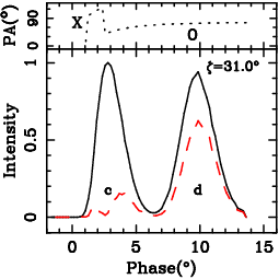
When a sight line has a small impact angle, , i.e., , cutting across pulsar emission beam, it will detect emissions from the density patches , , and in Fig. 5. The resulting pulse profiles are shown in Fig. 6, depending on the available density patch combinations, for example (, ) or (, ). We can conclude from simulations that:
1) The highly polarized components can be generated from the leading (patch ) and the trailing (patch ) parts of pulsar emission beam, both of which are dominated by the O-mode.
2) The highly polarized components have a flat polarization angle curve, because density patches and are away from the meridional plan of .
3) The low polarized components exhibit orthogonal modes, and the emission from the X and O modes has comparable intensity. Orthogonal mode jump happens when one mode dominates over the other, as shown by the polarization angle curves.
In addition, the simulations predict that the highly polarized components are more likely to be generated at the leading parts of pulse profiles, because the highly polarized leading part of pulsar emission beam is broader than the trailing one (see Fig.5) due to rotation-induced asymmetry. Highly polarized components would have a flatter spectrum than the low polarized components, because the beam regions further away from the magnetic axis tend to have a flat spectrum according to Lyne & Manchester (1988), while the detailed spectrum behavior is not modeled in our simulations.
3.3 Polarized pulse profiles obtained by a large impact angle
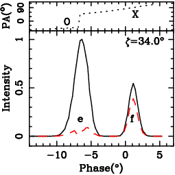


When a sight line has a large impact angle to cut across the pulsar emission beam, it will detect emission from density patches , and in Fig. 5. The resulting pulse profiles are shown in Fig. 7 for different patch combinations (, ), (, ) or (, , ) for available density distributions of particles. Highly polarized components can appear at the leading, central or trailing part of pulse profiles. These profiles have similar features as those in Fig. 6, but differences are as following.
1) The highly polarized component from the bottom part, i.e., density patch , of pulsar emission beam is dominated by the X-mode, rather than the O-mode.
2) Highly polarized component has a steeper polarization angle curve, because the component is generated near the meridional plane, where the polarization angle has the maximum rate of change approximating . The gradient is inversely proportional to the impact angle .
3) Highly polarized component may have a similar spectrum to the low polarized components, since all components are generated at comparable distances from the magnetic axis.
In summary, joint simulations of emission processes and propagation effects demonstrate that highly polarized components can be produced at the leading, central and trailing parts of pulse profiles. The properties of emission components, polarization angle curve, mode characteristic and spectrum, depend on pulsar geometry and the density patches of radiating particles.
4 Discussions and Conclusions
In this paper, we have investigated the highly polarized components of integrated pulse profiles observationally and theoretically. We found from observational data that:
(i) Highly polarized components of pulsar profiles have a flatter spectrum than the low polarized components, regardless of their locations at the leading or trailing phase;
(ii) Highly polarized components tend to have a flat polarization angle curve, though a small fraction of pulsars have very steep polarization angle curves;
(iii) Highly polarized components generally have one mode, while the low polarized components often show orthogonal modes;
(iv) Significant scattering will cause depolarization at the trailing parts of pulse profiles and result in flat polarization angle curves;
(v) Millisecond pulsars can have highly polarized components as normal pulsars.
We simulated emission processes and propagation effects within pulsar magnetosphere, and found that highly polarized emission could be produced at the leading (O-mode), trailing (O-mode), top (X-mode) and bottom (X-mode) parts of pulsar emission beam. When a sight line cuts across the beam with different impact angles, the detected highly polarized components have different properties, depending on the specific geometry and available density patches of the radiating particles:
(i) Highly polarized component generated from the leading or trailing part of pulsar emission beam is of the O-mode, and has a flat polarization angle curve;
(ii) Highly polarized component generated from the top or bottom part of pulsar emission beam is of the X-mode, and has a steep polarization angle curve.
In the observational aspect, polarization observations at multiple frequencies are important to reveal the frequency dependencies of intensities and polarization degrees of the components. The polarization observations should have higher signal to noise ratio and time resolution. For example, PSR J1048-5832 appeared to have one component at 1.44GHz due to limited time resolution (Qiao et al., 1995), but it is clearly resolved to two components by the recent polarization observations at 1.5GHz (Weltevrede & Johnston, 2008), which show clearly the gradient differences of polarization angle curves between the highly polarized and low polarized components. In addition, single pulse observations can help to identify the wave modes and depolarization processes (Stinebring et al., 1984a; Stinebring et al., 1984b).
In the theoretical aspect, our simulations here represent the further development of joint researches on the emission processes and propagation effects (Wang et al., 2014) and focus mainly on the properties for the highly polarized components within the wave mode separated magnetosphere. Note, however that in our current calculations, the magnetic field is assumed to be a rotating dipole for an empty magnetosphere. Radiation correction is neglected, and the effect of loaded plasma on magnetic fields is not yet incorporated. Furthermore, the energy and density distributions of relativistic particles are assumed to follow a simple model. Therefore, the conclusions and predictions under these assumptions may be altered if more complicated pulsar magnetosphere is considered.
Acknowledgements
This work has been supported by the National Natural Science Foundation of China (11403043, 11473034 and 11273029), and the Strategic Priority Research Programme “The Emergence of Cosmological Structures” of the Chinese Academy of Sciences (Grant No. XDB09010200).
References
- Backus et al. (2010) Backus I., Mitra D., Rankin J. M., 2010, MNRAS, 404, 30
- Barnard & Arons (1986) Barnard J. J., Arons J., 1986, ApJ, 302, 138
- Beskin & Philippov (2012) Beskin V. S., Philippov A. A., 2012, MNRAS, 425, 814
- Biggs et al. (1988) Biggs J. D., Lyne A. G., Hamilton P. A., McCulloch P. M., Manchester R. N., 1988, MNRAS, 235, 255
- Blaskiewicz et al. (1991) Blaskiewicz M., Cordes J. M., Wasserman I., 1991, ApJ, 370, 643
- Cheng & Ruderman (1979) Cheng A. F., Ruderman M. A., 1979, ApJ, 229, 348
- Connors et al. (2002) Connors T. W., Johnston S., Manchester R. N., McConnell D., 2002, MNRAS, 336, 1201
- Crawford & Keim (2003) Crawford F., Keim N. C., 2003, ApJ, 590, 1020
- Crawford et al. (2001) Crawford F., Manchester R. N., Kaspi V. M., 2001, AJ, 122, 2001
- Dai et al. (2015) Dai S., Hobbs G., Manchester R. N., Kerr, et. al., 2015, MNRAS, 449, 3223
- Demorest et al. (2004) Demorest P., Ramachandran R., Backer D. C., Ransom S. M., Kaspi V., Arons J., Spitkovsky A., 2004, ApJL, 615, L137
- Everett & Weisberg (2001) Everett J. E., Weisberg J. M., 2001, ApJ, 553, 341
- Force et al. (2015) Force M. M., Demorest P., Rankin J. M., 2015, MNRAS, 453, 4485
- Gaensler et al. (1998) Gaensler B. M., Stappers B. W., Frail D. A., Johnston S., 1998, ApJL, 499, L69
- Gangadhara (2010) Gangadhara R. T., 2010, ApJ, 710, 29
- Gould & Lyne (1998) Gould D. M., Lyne A. G., 1998, MNRAS, 301, 235
- Guillemot et al. (2013) Guillemot L., et al., 2013, ApJ, 768, 169
- Hamilton et al. (1977) Hamilton P. A., McCulloch P. M., Ables J. G., Komesaroff M. M., 1977, MNRAS, 180, 1
- Han et al. (2009) Han J. L., Demorest P. B., van Straten W., Lyne A. G., 2009, ApJS, 181, 557
- Hankins & Rankin (2010) Hankins T. H., Rankin J. M., 2010, AJ, 139, 168
- Hotan et al. (2004) Hotan A. W., Bailes M., Ord S. M., 2004, MNRAS, 355, 941
- Hotan et al. (2005) Hotan A. W., Bailes M., Ord S. M., 2005, MNRAS, 362, 1267
- Johnston & Weisberg (2006) Johnston S., Weisberg J. M., 2006, MNRAS, 368, 1856
- Johnston et al. (1996) Johnston S., Manchester R. N., Lyne A. G., D’Amico N., Bailes M., Gaensler B. M., Nicastro L., 1996, MNRAS, 279, 1026
- Johnston et al. (2005) Johnston S., Hobbs G., Vigeland S., Kramer M., Weisberg J. M., Lyne A. G., 2005, MNRAS, 364, 1397
- Johnston et al. (2006) Johnston S., Karastergiou A., Willett K., 2006, MNRAS, 369, 1916
- Johnston et al. (2007) Johnston S., Kramer M., Karastergiou A., Hobbs G., Ord S., Wallman J., 2007, MNRAS, 381, 1625
- Johnston et al. (2008) Johnston S., Karastergiou A., Mitra D., Gupta Y., 2008, MNRAS, 388, 261
- Karastergiou & Johnston (2004) Karastergiou A., Johnston S., 2004, MNRAS, 352, 689
- Karastergiou & Johnston (2006) Karastergiou A., Johnston S., 2006, MNRAS, 365, 353
- Karastergiou et al. (2005) Karastergiou A., Johnston S., Manchester R. N., 2005, MNRAS, 359, 481
- Keith et al. (2008) Keith M. J., Johnston S., Kramer M., Weltevrede P., Watters K. P., Stappers B. W., 2008, MNRAS, 389, 1881
- Keith et al. (2011) Keith M. J., Johnston S., Levin L., Bailes M., 2011, MNRAS, 416, 346
- Keith et al. (2013) Keith M. J., Shannon R. M., Johnston S., 2013, MNRAS, 432, 3080
- Komesaroff et al. (1974) Komesaroff M. M., McCulloch P. M., Rankin J. M., 1974, Nature, 252, 210
- Kramer & Johnston (2008) Kramer M., Johnston S., 2008, MNRAS, 390, 87
- Kramer et al. (1994) Kramer M., Wielebinski R., Jessner A., Gil J. A., Seiradakis J. H., 1994, A&AS, 107, 515
- Kramer et al. (1999) Kramer M., et al., 1999, ApJ, 520, 324
- Kramer et al. (2002) Kramer M., Johnston S., van Straten W., 2002, MNRAS, 334, 523
- Krishnamohan & Downs (1983) Krishnamohan S., Downs G. S., 1983, ApJ, 265, 372
- Li & Han (2003) Li X. H., Han J. L., 2003, A&A, 410, 253
- Liu et al. (2015) Liu K., et al., 2015, MNRAS, 449, 1158
- Lyne & Manchester (1988) Lyne A. G., Manchester R. N., 1988, MNRAS, 234, 477
- Lyne et al. (1971) Lyne A. G., Smith F. G., Graham D. A., 1971, MNRAS, 153, 337
- Manchester (1971) Manchester R. N., 1971, ApJS, 23, 283
- Manchester & Johnston (1995) Manchester R. N., Johnston S., 1995, ApJL, 441, L65
- Manchester et al. (1980) Manchester R. N., Hamilton P. A., McCulloch P. M., 1980, MNRAS, 192, 153
- Manchester et al. (1998) Manchester R. N., Han J. L., Qiao G. J., 1998, MNRAS, 295, 280
- McCulloch et al. (1976) McCulloch P. M., Hamilton P. A., Ables J. G., Komesaroff M. M., 1976, MNRAS, 175, 71P
- McCulloch et al. (1978) McCulloch P. M., Hamilton P. A., Manchester R. N., Ables J. G., 1978, MNRAS, 183, 645
- McKinnon (2004) McKinnon M. M., 2004, ApJ, 606, 1154
- McLaughlin & Rankin (2004) McLaughlin M. A., Rankin J. M., 2004, MNRAS, 351, 808
- Mitra & Rankin (2011) Mitra D., Rankin J. M., 2011, ApJ, 727, 92
- Morris et al. (1980) Morris D., Sieber W., Ferguson D. C., Bartel N., 1980, A&A, 84, 260
- Morris et al. (1981) Morris D., Graham D. A., Sieber W., Bartel N., Thomasson P., 1981, A&AS, 46, 421
- Noutsos et al. (2009) Noutsos A., Karastergiou A., Kramer M., Johnston S., Stappers B. W., 2009, MNRAS, 396, 1559
- Noutsos et al. (2012) Noutsos A., Kramer M., Carr P., Johnston S., 2012, MNRAS, 423, 2736
- Noutsos et al. (2015) Noutsos A., Sobey C., Kondratiev V. I., Weltevrede, et. al, 2015, A&A, 576, A62
- O’Brien et al. (2008) O’Brien J. T., Johnston S., Kramer M., Lyne, et. al., 2008, MNRAS, 388, L1
- Ord et al. (2004) Ord S. M., van Straten W., Hotan A. W., Bailes M., 2004, MNRAS, 352, 804
- Phillips (1990) Phillips J. A., 1990, ApJL, 361, L57
- Qiao et al. (1995) Qiao G., Manchester R. N., Lyne A. G., Gould D. M., 1995, MNRAS, 274, 572
- Ramachandran & Kramer (2003) Ramachandran R., Kramer M., 2003, A&A, 407, 1085
- Ramachandran et al. (2002) Ramachandran R., Rankin J. M., Stappers B. W., Kouwenhoven M. L. A., van Leeuwen A. G. J., 2002, A&A, 381, 993
- Rankin (1983) Rankin J. M., 1983, ApJ, 274, 333
- Rankin (2007) Rankin J. M., 2007, ApJ, 664, 443
- Rankin & Benson (1981) Rankin J. M., Benson J. M., 1981, AJ, 86, 418
- Rankin & Rathnasree (1997) Rankin J. M., Rathnasree N., 1997, Journal of Astrophysics and Astronomy, 18, 91
- Rankin et al. (1989) Rankin J. M., Stinebring D. R., Weisberg J. M., 1989, ApJ, 346, 869
- Rankin et al. (2005) Rankin J. M., Ramachandran R., Suleymanova S. A., 2005, A&A, 429, 999
- Rankin et al. (2006) Rankin J. M., Rodriguez C., Wright G. A. E., 2006, MNRAS, 370, 673
- Ransom et al. (2005) Ransom S., Demorest P., Kaspi V., Ramachandran R., Backer D., 2005, in Rasio F. A., Stairs I. H., eds, Astronomical Society of the Pacific Conference Series Vol. 328, Binary Radio Pulsars. p. 73 (arXiv:astro-ph/0404341)
- Roberts et al. (2001) Roberts M. S. E., Romani R. W., Johnston S., 2001, ApJL, 561, L187
- Rookyard et al. (2015) Rookyard S. C., Weltevrede P., Johnston S., 2015, MNRAS, 446, 3367
- Rosen & Demorest (2011) Rosen R., Demorest P., 2011, ApJ, 728, 156
- Sieber (1973) Sieber W., 1973, A&A, 28, 237
- Stairs et al. (1999) Stairs I. H., Thorsett S. E., Camilo F., 1999, ApJS, 123, 627
- Stinebring et al. (1984a) Stinebring D. R., Cordes J. M., Rankin J. M., Weisberg J. M., Boriakoff V., 1984a, ApJS, 55, 247
- Stinebring et al. (1984b) Stinebring D. R., Cordes J. M., Weisberg J. M., Rankin J. M., Boriakoff V., 1984b, ApJS, 55, 279
- Wang et al. (2001) Wang H. G., Han J. L., Qiao G. J., 2001, ChA&A, 25, 73
- Wang et al. (2010) Wang C., Lai D., Han J. L., 2010, MNRAS, 403, 569
- Wang et al. (2012) Wang P. F., Wang C., Han J. L., 2012, MNRAS, 423, 2464
- Wang et al. (2014) Wang P. F., Wang C., Han J. L., 2014, MNRAS, 441, 1943
- Wang et al. (2015) Wang P. F., Wang C., Han J. L., 2015, MNRAS, 448, 771
- Weisberg et al. (1999) Weisberg J. M., Cordes J. M., Lundgren S. C., Dawson, et. al., 1999, ApJS, 121, 171
- Weisberg et al. (2004) Weisberg J. M., Cordes J. M., Kuan B., Devine K. E., Green J. T., Backer D. C., 2004, ApJS, 150, 317
- Weltevrede & Johnston (2008) Weltevrede P., Johnston S., 2008, MNRAS, 391, 1210
- Weltevrede & Wright (2009) Weltevrede P., Wright G., 2009, MNRAS, 395, 2117
- Weltevrede et al. (2010) Weltevrede P., Abdo A. A., Ackermann M., , et. al. 2010, ApJ, 708, 1426
- Weltevrede et al. (2011) Weltevrede P., Johnston S., Espinoza C. M., 2011, MNRAS, 411, 1917
- Wu et al. (1993) Wu X. J., Manchester R. N., Lyne A. G., Qiao G., 1993, MNRAS, 261, 630
- Xilouris et al. (1991) Xilouris K. M., Rankin J. M., Seiradakis J. H., Sieber W., 1991, A&A, 241, 87
- Xilouris et al. (1995) Xilouris K. M., Seiradakis J. H., Gil J., Sieber W., Wielebinski R., 1995, A&A, 293, 153
- Xilouris et al. (1996) Xilouris K. M., Kramer M., Jessner A., Wielebinski R., Timofeev M., 1996, A&A, 309, 481
- Xilouris et al. (1998) Xilouris K. M., Kramer M., Jessner A., von Hoensbroech A., Lorimer D. R., Wielebinski R., Wolszczan A., Camilo F., 1998, ApJ, 501, 286
- Yan et al. (2011) Yan W. M., Manchester R. N., van Straten W., Reynolds, et. al., 2011, MNRAS, 414, 2087
- Zepka et al. (1996) Zepka A., Cordes J. M., Wasserman I., Lundgren S. C., 1996, ApJ, 456, 305
- van Ommen et al. (1997) van Ommen T. D., D’Alessandro F., Hamilton P. A., McCulloch P. M., 1997, MNRAS, 287, 307
- van Straten (2013) van Straten W., 2013, ApJS, 204, 13
- von Hoensbroech & Xilouris (1997) von Hoensbroech A., Xilouris K. M., 1997, A&AS, 126, 121
- von Hoensbroech et al. (1998) von Hoensbroech A., Kijak J., Krawczyk A., 1998, A&A, 334, 571
Appendix A Peak intensity ratios for highly and low polarized components
Tables 4 and 5 list the peak intensity ratios, , of the highly polarized components at the leading and trailing part of profiles with respect to the low polarized components at a series of frequencies.
| PSR | Freq.(GHz) | References | |
|---|---|---|---|
| J0358+5413 | 0.234 | 31 | |
| 0.325 | 77 | ||
| 0.408 | 16, 31 | ||
| 0.610 | 31 | ||
| 0.925 | 31 | ||
| 1.408 | 31 | ||
| 1.642 | 31 | ||
| 1.71 | 30 | ||
| 1.72 | 9, 20 | ||
| 2.65 | 8, 9 | ||
| 4.85 | 30, 34, 81 | ||
| 8.7 | 9 | ||
| 10.55 | 24, 30, 34 | ||
| 32.0 | 26 | ||
| J0454+5543 | 0.234 | 31 | |
| 0.408 | 16, 31 | ||
| 0.610 | 31 | ||
| 0.91 | 31 | ||
| 1.408 | 30, 31 | ||
| 1.642 | 31 | ||
| 1.72 | 20 | ||
| 4.85 | 30, 81 | ||
| J1048-5832 | 0.692 | 90 | |
| 1.369 | 90 | ||
| 1.5 | 69 | ||
| 3.0 | 69 | ||
| 3.1 | 56, 90 | ||
| 6.387 | 90 | ||
| 8.4 | 59, 90 | ||
| J1057-5226IP | 0.17 | 12 | |
| 0.325 | 77 | ||
| 0.631 | 6, 12 | ||
| 0.64 | 16 | ||
| 0.692 | 90 | ||
| 0.95 | 29 | ||
| 1.369 | 4, 72, 90 | ||
| 1.5 | 69 | ||
| 3.0 | 69, 90 | ||
| J1825-0935MP | 0.243 | 65 | |
| 0.325 | 65, 73, 77 | ||
| 0.408 | 31 | ||
| 0.61 | 31 | ||
| 0.69 | 63, 65 | ||
| 0.925 | 31 | ||
| 0.95 | 29 | ||
| 1.4 | 30, 49, 61, 65 | ||
| 1.612 | 7 | ||
| 3.1 | 61, 63, 65 | ||
| 4.85 | 30 | ||
| 10.45 | 30 | ||
| J1844+1454 | 0.243 | 65, 90 | |
| 0.325 | 65, 77, 90 | ||
| 0.408 | 31 | ||
| 0.61 | 31 | ||
| 0.69 | 65, 90 | ||
| 0.925 | 31 | ||
| 1.4 | 17, 31, 38 | ||
| 54, 65, 74 | |||
| 1.642 | 31 | ||
| 3.1 | 65, 90 |
Note: The highly polarized components of PSR J0358+5413 and J1844+1454 are confused with the corresponding low polarized components at frequencies smaller than 0.408 and 0.61GHz.
| PSR | Freq.(GHz) | References | |
| J0601-0527 | 0.243 | 90 | |
| 0.325 | 90 | ||
| 0.408 | 31 | ||
| 0.61 | 31 | ||
| 0.692 | 90 | ||
| 0.925 | 31 | ||
| 1.408 | 31, 54, 90 | ||
| 1.5 | 69 | ||
| 1.642 | 31 | ||
| 1.72 | 20 | ||
| 3.068 | 90 | ||
| 4.85 | 34 | ||
| 6.2 | 90 | ||
| J0922+0638 | 0.243 | 65, 90 | |
| 0.322 | 62, 65, 90 | ||
| 0.43 | 19 | ||
| 0.690 | 65, 90 | ||
| J1539-5626 | 0.692 | 90 | |
| 1.377 | 90 | ||
| 1.5 | 69 | ||
| 3.1 | 56, 69, 90 | ||
| 6.2 | 90 | ||
| 8.356 | 59, 90 | ||
| J2225+6535 | 0.15 | 88 | |
| 0.234 | 31 | ||
| 0.325 | 77 | ||
| 0.408 | 16, 31 | ||
| 0.61 | 31 | ||
| 0.925 | 31 | ||
| 1.408 | 31 | ||
| 1.5 | 86 | ||
| 1.642 | 31 | ||
| 1.7 | 9 |
Note: The highly polarized components of PSR J0922+0638 are confused with the low polarized components at frequencies larger than 0.69GHz.