跳到论文正文
W Papers独立论文阅读器 arXiv:1608.07173 论文正文 计算阅读时间 · 0%
引用这篇论文根据当前论文元数据生成,正式投稿前建议核对。


License: arXiv.org perpetual non-exclusive license
arXiv:1608.07173v4 [stat.ME] 30 Aug 2017

Supplement to
multiscale blind source separation

Merle Behr??,??    Chris Holmes??,??    Axel Munk??,??,??    Merle Behr??    Chris Holmes??    Axel Munk??,??

We provide a new methodology for statistical recovery of single linear mixtures of piecewise constant signals (sources) with unknown mixing weights and change points in a multiscale fashion. We show exact recovery within an ϵ\epsilon-neighborhood of the mixture when the sources take only values in a known finite alphabet. Based on this we provide the SLAM (Separates Linear Alphabet Mixtures) estimators for the mixing weights and sources. For Gaussian error, we obtain uniform confidence sets and optimal rates (up to log-factors) for all quantities. SLAM is efficiently computed as a nonconvex optimization problem by a dynamic program tailored to the finite alphabet assumption. Its performance is investigated in a simulation study. Finally, it is applied to assign copy-number aberrations from genetic sequencing data to different clones and to estimate their proportions.

, ,  and

University of Goettingen ??, University of Oxford ??,
and Max Planck Institute for Biophysical Chemistry ??

1 Introduction

As the presented methodology requires a quite broad range of techniques we will briefly introduce them in this section for explanatory purposes. Details are given in subsequent sections and a supplement.

1.1 The statistical blind source separation problem

We will start by introducing a particular kind of the blind source separation (BSS) problem which will be considered throughout this paper. More generally, in BSS problems (for a review see Section 1.8) one observes a mixture of signals (sources) and aims to recover these sources from the available observations, usually corrupted by noise. The blindness refers to the fact that neither the sources nor the mixing weights are known. Of course, without any additional information on the sources the BSS problem is unsolvable as the weights and sources cannot be separated, in general. However, under the additional assumption that the sources take values in a known finite alphabet, we will show that estimation of all quantities and inference for these is indeed possible.

Motivated by several applications mainly from digital communications (e.g., the recovery of mixtures of multi-level PAM signals (see [69, 55])) and cancer genetics (see Section 1.7), we assume, from now on, that the mm source functions fi,f^{i}, i=1,…,mi=1,\ldots,m, consist of arrays of constant segments, that is, step functions with unknown jump sizes, numbers, and locations of change points (c.p.’s), respectively. More specifically, let for a finite (known) ordered alphabet 𝔄={a1,…,ak}⊂ℝ\mathfrak{A}=\{a_{1},\ldots,a_{k}\}\subset\mathds{R}, with a1<…<aka_{1}<\ldots<a_{k}, each source function be in the class of step functions on [0,1)[0,1)

𝒮(𝔄):⁣={∑j=0Kθj𝟙[τj,τj+1):θj∈𝔄,0=τ0<…<τK<τK+1=1,K∈ℕ}.\small\mathcal{S}(\mathfrak{A})\mathrel{\mathop{:}\!\!=}\Big\{\sum_{j=0}^{K}\theta_{j}\mathds{1}_{[\tau_{j},\tau_{j+1})}:\theta_{j}\in\mathfrak{A},0=\tau_{0}<...<\tau_{K}<\tau_{K+1}=1,K\in\mathds{N}\Big\}. (1)

Note that this implies that for each source function the number K⁡(fi)K(f^{i}) of c.p.’s is assumed to be finite, possibly different, and unknown. We will assume θj≠θj+1\theta_{j}\neq\theta_{j+1} for j=0,…,Kj=0,...,K to ensure identifiability of the c.p.’s τj\tau_{j}. Note that without further specification 𝒮:⁣=𝒮(𝔄)\mathcal{S}\mathrel{\mathop{:}\!\!=}\mathcal{S}(\mathfrak{A}) is an extremely flexible class of functions, including any discretized source function taking values in 𝔄\mathfrak{A}. Moreover, we define the set of all possible (linear) mixtures with mm components each in 𝒮\mathcal{S} as

ℳ:⁣=ℳ(𝔄,m)={ω⊤f=∑i=1mωifi:ω∈Ω(m) and f∈𝒮(𝔄)m},\mathcal{M}\mathrel{\mathop{:}\!\!=}\mathcal{M}(\mathfrak{A},m)=\Big\{\omega^{\top}f=\sum_{i=1}^{m}\omega_{i}f^{i}:\omega\in\Omega(m)\text{ and }f\in\mathcal{S}(\mathfrak{A})^{m}\Big\}, (2)

with mixing weights ω\omega in the mm-simplex

Ω(m):⁣={ω∈ℝm:0≤ω1≤…≤ωm and ∑i=1mωi=1}.\Omega(m)\mathrel{\mathop{:}\!\!=}\big\{\omega\in\mathds{R}^{m}:0\leq\omega_{1}\leq\ldots\leq\omega_{m}\text{ and }\sum_{i=1}^{m}\omega_{i}=1\big\}. (3)

For a set Ω~⊂Ω⁡(m)\tilde{\Omega}\subset\Omega(m) we define ℳ⁡(𝔄,Ω~)\mathcal{M}(\mathfrak{A},\tilde{\Omega}) analogously. Throughout the following we assume that mm is known. Extension to unknown mm is akin to a model selection type of problem and beyond the scope of this paper.

In summary, in this paper we will be concerned with the statistical blind source separation regression model.

The SBSSR-model For a given finite alphabet 𝔄\mathfrak{A} and a given number of mixture components m∈ℕm\in\mathds{N} let g=∑i=1mωi​fi∈ℳg=\sum_{i=1}^{m}\omega_{i}f^{i}\in\mathcal{M} be an arbitrary mixture of mm piecewise constant source functions fi∈𝒮f^{i}\in\mathcal{S}. Suppose we observe

Yj=g(xj)+σϵj,j=1,…,n,Y_{j}=g(x_{j})+\sigma\epsilon_{j},\qquad j=1,\ldots,n, (4)

at sampling points xj:⁣=(j−1)/nx_{j}\mathrel{\mathop{:}\!\!=}(j-1)/n, s.t. the error (ϵ1,…,ϵn)⊤∼𝒩⁡(0,In)(\epsilon_{1},...,\epsilon_{n})^{\top}\sim\mathcal{N}(0,I_{n}), σ>0\sigma>0, that is, i.i.d. centered normal random variables with variance σ2\sigma^{2}.

Example 1.1.

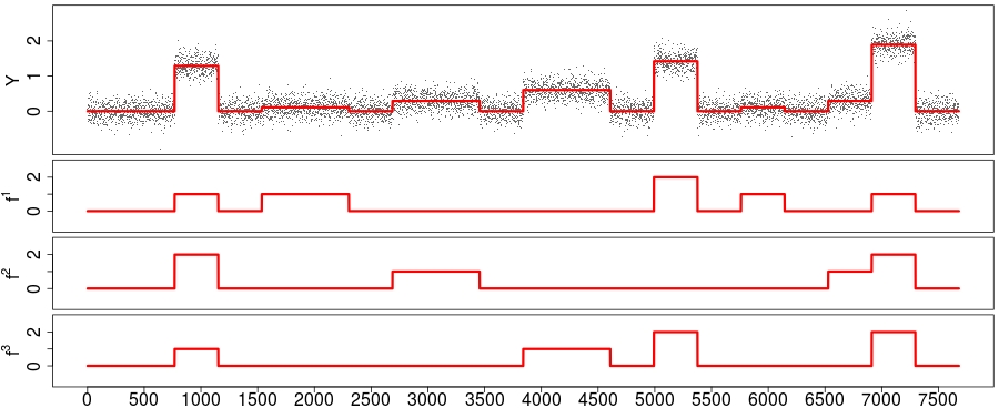
In Figure 1.1, a mixture gg of m=3m=3 source functions f1f^{1}, f2f^{2}, f3f^{3}, taking values in the alphabet 𝔄={0,1,2}\mathfrak{A}=\{0,1,2\}, is displayed. The mixing weights are given by ω⊤=(0.11,0.29,0.6)\omega^{\top}=(0.11,0.29,0.6). Normal noise with standard deviation σ=0.22\sigma=0.22 is added according to the SBSSR-model, n=7680n=7680. Both, nn and σ\sigma were chosen close to our data example in Section 5.

Refer to caption
Fig 1.1: The mixture g=0.11​f1+0.29​f2+0.6​f3g=0.11f^{1}+0.29f^{2}+0.6f^{3}, together with the observations YY (gray dots), and the sources f1f^{1}, f2f^{2}, f3f^{3} from Example 1.1 (from top to bottom).

In summary, the unknowns in the SBSSR-model are

  1. 1.

    the weights ω=(ω1,…,ωm)⊤\omega=(\omega_{1},\ldots,\omega_{m})^{\top} and

  2. 2.

    the source functions fif^{i}, i=1,…,mi=1,\ldots,m, i.e. their

    1. (a)

      number of c.p.’s K⁡(fi)K(f^{i}),

    2. (b)

      c.p. locations τji\tau_{j}^{i}, j=1,…,K⁡(fi)j=1,\ldots,K(f^{i}), and

    3. (c)

      function values fi​(x)f^{i}(x) (∈𝔄\in\mathfrak{A}) at locations x∈[0,1)x\in[0,1).

In this paper we will address estimation of all the quantities in 1. and 2. and, in addition, we will construct under further assumptions

  1. 3.

    a uniform (i.e., honest) confidence region 𝒞1−α\mathcal{C}_{1-\alpha} for the weights ω\omega and

  2. 4.

    asymptotically uniform multivariate confidence bands for the source functions f=(f1,…,fm)⊤f=(f^{1},\ldots,f^{m})^{\top}.

Remark 1.1.
  1. a)

    For simplicity, we assume throughout the following that gg in (4) is sampled equidistantly at xj=(j−1)/nx_{j}=(j-1)/n, j=1,…,nj=1,\ldots,n and that all functions are defined on the domain [0,1)[0,1). We stress that extensions to more general domains ⊆ℝ\subseteq\mathds{R} and sampling designs are straightforward under suitable assumptions (see, e.g., [10]) but will be suppressed to ease notation.

  2. b)

    Further, for sake of brevity, we will assume that in (4) the variance σ2\sigma^{2} is known, otherwise one may pre-estimate it n\sqrt{n}-consistently by standard methods, see, for example, [49, 38, 20, 19] and Section 5.

1.2 Identifiability and exact recovery

Before we introduce estimators for ω\omega and ff, we need to discuss identifiability of these parameters in the SBSSR-model, that is, conditions when gg determines them uniquely via g=∑i=1mωi​fig=\sum_{i=1}^{m}\omega_{i}f^{i}.

Although, deterministic finite alphabet instantaneous (linear) mixtures, i.e., σ=0\sigma=0 in the SBSSR-model (4), received a lot of attention in the literature [66, 53, 72, 21, 42, 36, 58], a complete characterization of identifiability remained elusive and has been recently provided in [5], which will be briefly reviewed here as far as it is required for our purposes. Obviously, not every mixture g∈ℳg\in\mathcal{M} in (2) is identifiable. Consider, for example, ω∈Ω⁡(m)\omega\in\Omega(m) in (3) such that ω1=ω2\omega_{1}=\omega_{2}. Then a jump in the source function f1f^{1} has the same effect on the mixture gg as a jump in f2f^{2} and hence, f1f^{1} and f2f^{2} cannot be distinguished from the mixture gg. Likewise, when ω1\omega_{1} and ω2\omega_{2} are close, i.e., ω2−ω1→0\omega_{2}-\omega_{1}\rightarrow 0, it becomes arbitrarily difficult to separate f1f^{1} and f2f^{2} from the observations YY in the SBSSR-model. For statistical estimation, it is therefore necessary that different source function values f⁡(x)=(f1​(x),…,fm​(x))∈𝔄mf(x)=(f^{1}(x),\ldots,f^{m}(x))\in\mathfrak{A}^{m} are sufficiently well separated by the mixing weights ω\omega. This is quantified by the alphabet separation boundary [5]

ASB(ω)=ASB(ω,𝔄):⁣=mina≠a′∈𝔄m|ω⊤a−ω⊤a′|.\displaystyle ASB(\omega)=ASB(\omega,\mathfrak{A})\mathrel{\mathop{:}\!\!=}\min_{a\neq a^{\prime}\in\mathfrak{A}^{m}}\left|\omega^{\top}a-\omega^{\top}a^{\prime}\right|. (5)

A necessary identifiability condition in the SBSSR-model is A​S​B​(ω)>0ASB(\omega)>0 (see [5, Section 3.A]), where the size of A​S​B​(ω)ASB(\omega) can be understood as a conditioning number for the difficulty of separating the sources in the SBSSR-model, that is, the smaller A​S​B​(ω)ASB(\omega), the more difficult separation of sources. Therefore, to quantify the estimation error of any method which serves the purposes in 1. - 4. we must restrict to submodels of mixing weights which sufficiently separate different alphabet values in 𝔄m\mathfrak{A}^{m}, that is, for given δ>0\delta>0 we introduce

Ωδ=Ωδ(𝔄,m):⁣={ω∈Ω(m):ASB(ω)≥δ}.\Omega^{\delta}=\Omega^{\delta}(\mathfrak{A},m)\mathrel{\mathop{:}\!\!=}\big\{\omega\in\Omega(m):ASB(\omega)\geq\delta\}. (6)

Note further that A​S​B​(ω)>0ASB(\omega)>0 implies that any jump in the source vector ff (i.e., at least one source fif^{i} jumps) occurs as well in the mixture g=ω⊤​fg=\omega^{\top}f and that A​S​B​(ω)ASB(\omega) coincides with the minimal possible jump height of gg.

Just as we have restricted the possible ω\omega’s in (6), it is necessary to further restrict the set of possible source functions f∈𝒮​(𝔄)mf\in\mathcal{S}(\mathfrak{A})^{m} in (1). Consider for example the case of two sources, m=2m=2, such that f1=f2f^{1}=f^{2}. Then g=ω1​f1+ω2​f2=f1g=\omega_{1}f^{1}+\omega_{2}f^{2}=f^{1}, independently of ω\omega, and hence, ω\omega cannot be determined from gg. Therefore, a certain kind of variability of the sources fif^{i} is necessary to ensure identifiability of the mixing weights ω\omega. We employ from [5] the following simple sufficient identifiability condition.

Definition 1.2.

A vector of source functions f=(f1,…,fm)⊤∈𝒮​(𝔄)mf=(f^{1},\ldots,f^{m})^{\top}\in\mathcal{S}(\mathfrak{A})^{m} is separable if there exit intervals I1,…,Im⊂[0,1)I_{1},\ldots,I_{m}\subset[0,1) such that ff is constant on IrI_{r} with function values

f|Ir≡[A]r,r=1,…,m,f|_{I_{r}}\equiv[A]_{r},\qquad r=1,\ldots,m, (7)

with

A:⁣=a1Em+(a2−a1)Im=(a2a1a1…a1a1a2a1…a1a1a1…a1a2)∈𝔄m×m,A\mathrel{\mathop{:}\!\!=}a_{1}E_{m}+(a_{2}-a_{1})I_{m}=\begin{pmatrix}a_{2}&a_{1}&a_{1}&\ldots&a_{1}\\ a_{1}&a_{2}&a_{1}&\ldots&a_{1}\\ \vdots&&&&\vdots\\ a_{1}&a_{1}&\ldots&a_{1}&a_{2}\end{pmatrix}\in\mathfrak{A}^{m\times m}, (8)

where EmE_{m} denotes the matrix of ones, ImI_{m} the identity matrix, and [A]r[A]_{r} the rr-th row of AA.

The notation “separable” is borrowed from identifiability conditions for nonnegative matrix factorization [23, 2, 56], see Section 1.8 for details. Separability in Definition 1.2 means that for each of the mm sources fif^{i} there is a region where only this source function is “active” (taking the second smallest alphabet value a2a_{2}) and all the other sources are “silent” (taking the smallest alphabet value a1a_{1}). For example, if we have an alphabet of the form 𝔄={0,1,a3,…,ak}\mathfrak{A}=\{0,1,a_{3},...,a_{k}\}, AA becomes the identity matrix and separability means that each of the mixing weights ωi\omega_{i} appears at least once in the mixture g=ω⊤​fg=\omega^{\top}f. Note that separability in Definition 1.2 only requires that the values [A]r∈𝔄m[A]_{r}\in\mathfrak{A}^{m} are attained somewhere by the source functions f1,…,fmf^{1},\ldots,f^{m} and does not specify the location. For specific situations it is possible to replace the matrix AA in (8) by a different invertible (as a function from Ω⁡(m)\Omega(m) to ℝm\mathds{R}^{m}) matrix if this matrix induces enough variability in the sources for the weights to be identifiable from their mixture (see [5]). Here, however, we consider arbitrary alphabets and number of sources and the separability condition in Definition 1.2 ensures identifiability for arbitrary 𝔄\mathfrak{A} and mm, in general. Note that when the source functions f=(f1,…,fm)⊤f=(f^{1},\ldots,f^{m})^{\top} attain all kmk^{m} possible function values in 𝔄m\mathfrak{A}^{m} somewhere in [0,1)[0,1), the case of maximal variation, then, in particular, ff is separable (see [5] for further examples). We stress that the above assumption (7) on the variability of ff is close to being necessary for identifiability (see [5, Theorem 3.1]). Hence, without such an assumption no method can provide a unique decomposition of gg into the fif^{i}’s and its weights ωi\omega_{i}, i=1,…,mi=1,\ldots,m, even in the noiseless case. Summing up, we will, in the following, restrict to those mixtures gg in the SBSSR-model, which are in

ℳδ:⁣={ω⊤f=∑i=1mωifi:ω∈Ωδ and f∈𝒮(𝔄)m is separable}.\mathcal{M}^{\delta}\mathrel{\mathop{:}\!\!=}\Big\{\omega^{\top}f=\sum_{i=1}^{m}\omega_{i}f^{i}:\omega\in\Omega^{\delta}\text{ and }f\in\mathcal{S}(\mathfrak{A})^{m}\text{ is separable}\Big\}. (9)

For instance, in Example 1.1 ff is separable and ω∈Ω0.02\omega\in\Omega^{0.02}, i.e., g∈ℳ0.02g\in\mathcal{M}^{0.02}.

The following simple but fundamental result will guide us later on to derive estimators for all quantities in 1. and 2. in the statistical setting (4) (see Section 1.4).

Theorem 1.3 (Stable recovery of weights and source functions).

Let g=ω⊤​f,g~=ω~⊤​f~g=\omega^{\top}f,\tilde{g}=\tilde{\omega}^{\top}\tilde{f} be two mixtures in ℳδ\mathcal{M}^{\delta} for some δ>0\delta>0 and let ϵ\epsilon be such that 0<ϵ<δ⁡(a2−a1)/(2​m​(ak−a1))0<\epsilon<\delta(a_{2}-a_{1})/(2m(a_{k}-a_{1})). If

supx∈[0,1)|g⁡(x)−g~​(x)|<ϵ,\sup_{x\in[0,1)}\left|g(x)-\tilde{g}(x)\right|<\epsilon, (10)
  1. 1.

    then the weights satisfy the stable approximate recovery (SAR) property maxi=1,…,m⁡|ωi−ω~i|<ϵ/(a2−a1)\max_{i=1,\ldots,m}\left|\omega_{i}-\tilde{\omega}_{i}\right|<\epsilon/(a_{2}-a_{1}) and

  2. 2.

    the sources satisfy the stable exact recovery (SER) property f=f~f=\tilde{f}.

For a proof see Section S1.1 in the supplement.

1.3 Methodology: first approaches

In order to motivate our (quite involved) methodology, let us discuss briefly some attempts which may come to mind at a first glance. As a first approach to estimate ω\omega and ff from the data YY in the SBSSR-model one might pre-estimate the mixture gg with some standard c.p. procedure, ignoring its underlying mixture structure, and then try to reconstruct ω\omega and ff afterwards. One problem is that the resulting step function cannot be decomposed into mixing weights ω∈Ω⁡(m)\omega\in\Omega(m) and source function f∈𝒮m​(𝔄)f\in\mathcal{S}^{m}(\mathfrak{A}), in general, as the given alphabet 𝔄\mathfrak{A} leads to restrictions on the function values of gg. But already for the initial step of reconstructing the mixture gg itself, a standard c.p. estimation procedure (which does ignore the mixture structure) is unfavorable as it discards important information on the possible function values of gg (induced by 𝔄\mathfrak{A}). For example, if gg has a small jump in some region, this might be easily missed (see Figure 1.2 for an example). Consequently, subsequent estimation of ff and ω\omega will fail as well. In contrast, a procedure which takes the mixture structure explicitly into account right from its beginning is expected to have better detection power for a jump. As a conclusion, considering the SBSSR-model as a standard c.p. model discards important information and does not allow for demixing, in general.

Refer to caption
Fig 1.2: Observations YY from Example 1.1 (gray dots), together with the true underlying mixture gg (red line). The blue line shows the c.p. estimate from [31], which does not incorporate the mixture structure. The red line shows the estimate with the proposed method (see Figure 1.4 for the underlying recovery of ω\omega and the sources ff). The blue areas display a region where gg has a small jump (red line), which is not detected by the c.p. estimator [31] (blue line), but by the proposed method (black line). The bottom plots show a zoom in of the blue regions.

A second approach which comes to mind is to first use some clustering algorithm to pre-estimate the function values of gg, ignoring its serial c.p. structure, and infer the mixing weights ω\omega from this. This pre-clustering approach has been pursued in several papers [21, 72, 36] for the particular case of a binary alphabet, that is, k=2k=2. However, as the number of possible function values of gg equals kmk^{m} (recall that kk is the size of the alphabet and mm is the number of sources), recovery of these values in a statistical context by clustering is a difficult task in general, as it amounts to estimate the location of (at most) kmk^{m} modes correctly from the marginal distributions of the observations YjY_{j}. In fact, this corresponds to mode hunting (see, e.g., [54, 15, 67, 45, 29, 52]) with potentially large number of modes which is known to be a hard problem. We illustrate the difficulty of this in Figure 1.3 employing histograms of the YjY_{j}’s in Example 1.1 with different bin widths. From this, it becomes obvious that a pre-clustering approach is not feasible for the present data.

Refer to caption
Fig 1.3: Histogram of the data from Example 1.1 with 2020, 100100, and 200200 equidistant bins, respectively (from left to right). The vertical red lines indicate the true function values (modes) of gg which have to be identified.

Summing up, ignoring either of both, the c.p. and the finite alphabet mixture structure, in a first pre-estimation step discards important information which is indispensable for statistically efficient recovery. We emphasize that we are not aware of any existing method taking both aspects into account, in contrast to the method presented in this paper (SLAM), which will be briefly described now.

1.4 Separate Linear Alphabet Mixtures (SLAM)

In a first step, we will construct a confidence region 𝒞1−α\mathcal{C}_{1-\alpha} for the weights ω\omega which can be characterized by the acceptance region of a specific multiscale test with test statistic TnT_{n}, which is particularly well suited to capture both, the c.p. and the mixture structure, of gg. The confidence level is determined by a threshold qn​(α)q_{n}(\alpha) such that for any g=∑i=1mωi​fi∈ℳδg=\sum_{i=1}^{m}\omega_{i}f^{i}\in\mathcal{M}^{\delta}

{ω∈𝒞1−α(Y)}⊇{Tn≤qn(α)}.\{\omega\in\mathcal{C}_{1-\alpha}(Y)\}\supseteq\{T_{n}\leq q_{n}(\alpha)\}. (11)

In a second step we estimate ff based on a multiscale constraint again. In the following section we will introduce this procedure in more detail. We stress that the multiscale approach underlying SLAM is crucial for valid recovery of sources and mixing weights as the jumps potentially can occur at any location and any scale (i.e., interval length of neighboring sampling points).

1.4.1 Multiscale statistic and confidence boxes underlying SLAM

As the jump locations may occur at any place, a well established way for inferring the function values of gg is to use local log-likelihood ratio test statistics in a multiscale fashion (see e.g., [62, 28, 19, 29, 31]). Let g|[xi,xj]≡gi​jg|_{[x_{i},x_{j}]}\equiv g_{ij} denote that gg is constant on [xi,xj][x_{i},x_{j}] with function value gi​jg_{ij}. For the local testing problem on the interval [xi,xj]⊂[0,1)[x_{i},x_{j}]\subset[0,1) with some given value gi​j∈ℝg_{ij}\in\mathds{R}

H0:g|[xi,xj]≡gi​jvs.H1:g|[xi,xj]≢gi​jH_{0}:g|_{[x_{i},x_{j}]}\equiv g_{ij}\quad\text{vs.}\quad H_{1}:g|_{[x_{i},x_{j}]}\not\equiv g_{ij} (12)

the local log-likelihood ratio test statistic is

Tij​(Yi,…,Yj,gi​j)=ln⁡(supθ∈ℝ∏l=ijϕθ​(Yl)∏l=ijϕgi​j​(Yl))=(∑l=ijYl−gi​j)22​σ2​(j−i+1),T_{i}^{j}(Y_{i},\ldots,Y_{j},g_{ij})=\ln\left(\frac{\sup_{\theta\in\mathds{R}}\prod_{l=i}^{j}\phi_{\theta}(Y_{l})}{\prod_{l=i}^{j}\phi_{g_{ij}}(Y_{l})}\right)=\frac{(\sum_{l=i}^{j}Y_{l}-g_{ij})^{2}}{2\sigma^{2}(j-i+1)}, (13)

where ϕθ\phi_{\theta} denotes the density of the normal distribution with mean θ\theta and variance σ2\sigma^{2}. We then combine the local testing problems in (12) and define in our context the multiscale statistic TnT_{n} for some candidate function g~\tilde{g} (which may depend on YY) as

Tn(Y,g~):⁣=max1≤i≤j≤ng~|[xi,xj]≡g~i​j|∑l=ijYl−g~i​j|σ​j−i+1−pen(j−i+1),T_{n}(Y,\tilde{g})\mathrel{\mathop{:}\!\!=}\max_{\begin{subarray}{c}1\leq i\leq j\leq n\\ \tilde{g}|_{[x_{i},x_{j}]}\equiv\tilde{g}_{ij}\end{subarray}}\frac{|\sum_{l=i}^{j}Y_{l}-\tilde{g}_{ij}|}{\sigma\sqrt{j-i+1}}-pen(j-i+1), (14)

where pen(j−i+1):⁣=2​(ln⁡(n/(j−i+1))+1)pen(j-i+1)\mathrel{\mathop{:}\!\!=}\sqrt{2\left(\ln\left(n/(j-i+1)\right)+1\right)}. The maximum in (14) is understood to be taken only over those intervals [xi,xj][x_{i},x_{j}] on which g~\tilde{g} is constant with value g~i​j=g~​(xi)\tilde{g}_{ij}=\tilde{g}(x_{i}). The function values of g~\tilde{g} determine the local testing problems (the value gi​jg_{ij} in (12)) on the single scales [xi,xj][x_{i},x_{j}]. The calibration term p​e​n​(⋅)pen(\cdot) serves as a balancing of the different scales in a way that the maximum in (14) is equally likely attained on all scales (see [28, 31]). Other scale penalizations can be employed as well (see e.g., [70]), but, for the ease of brevity, will not be discussed here. With the notation Y¯ij:⁣=∑l=ijYl/(j−i+1)\bar{Y}_{i}^{j}\mathrel{\mathop{:}\!\!=}\sum_{l=i}^{j}Y_{l}/(j-i+1), the statistic Tn​(Y,g~)T_{n}(Y,\tilde{g}) in (14) has the following geometric interpretation:

Tn​(Y,g~)≤q⇔g~i​j∈B⁡(i,j)​∀1≤i≤j≤n​ with ​g~|[xi,xj]≡g~i​j,T_{n}(Y,\tilde{g})\leq q\;\Leftrightarrow\tilde{g}_{ij}\in B(i,j)\;\forall 1\leq i\leq j\leq n\text{ with }\tilde{g}|_{[x_{i},x_{j}]}\equiv\tilde{g}_{ij}, (15)

for q∈ℝq\in\mathds{R}, with intervals

B(i,j):⁣=[Y¯ij−q+p​e​n​(j−i+1)j−i+1/σ,Y¯ij+q+p​e​n​(j−i+1)j−i+1/σ].B(i,j)\mathrel{\mathop{:}\!\!=}\bigg[\overline{Y}_{i}^{j}-\frac{q+pen(j-i+1)}{\sqrt{j-i+1}/\sigma},\overline{Y}_{i}^{j}+\frac{q+pen(j-i+1)}{\sqrt{j-i+1}/\sigma}\bigg]. (16)

In the following we will make use of the fact that the distribution of Tn​(Y,g)T_{n}(Y,g), with g∈ℳδg\in\mathcal{M}^{\delta} (see (9)) the true signal from the SBSSR-model, can be bounded from above with that of Tn=Tn​(Y,0)T_{n}=T_{n}(Y,0). It is known that Tn​⇒𝒟​L​(𝔹)<∞T_{n}\overset{\mathcal{D}}{\Rightarrow}L(\mathds{B})<\infty a.s. as n→∞n\rightarrow\infty, a certain functional of the Brownian motion 𝔹\mathds{B} (see [28, 27]). Note that the distribution of Tn​(Y,0)T_{n}(Y,0) does not depend on the (unknown) ff and ω\omega anymore. As this distribution is not explicitly accessible and to be more accurate for small nn (≤5000\leq 5000 say) the finite sample distribution of TnT_{n} can be easily obtained by Monte Carlo simulations. From this one obtains qn​(α)q_{n}(\alpha), α∈(0,1)\alpha\in(0,1), the 1−α1-\alpha quantile of TnT_{n}. We then obtain

infg∈ℳδP​(Tn​(Y,g)≤qn​(α))≥1−α.\inf_{g\in\mathcal{M}^{\delta}}\textbf{P}(T_{n}(Y,g)\leq q_{n}(\alpha))\geq 1-\alpha. (17)

Hence, for the intervals in (16) with q=qn​(α)q=q_{n}(\alpha) it follows that for all g∈ℳδg\in\mathcal{M}^{\delta}

P​(gi​j∈B⁡(i,j)​∀1≤i≤j≤n​ with ​g|[xi,xj]≡gi​j)≥1−α.\textbf{P}(g_{ij}\in B(i,j)\;\forall 1\leq i\leq j\leq n\text{ with }g|_{[x_{i},x_{j}]}\equiv g_{ij})\geq 1-\alpha. (18)

In the following, we use the notation B⁡(i,j)B(i,j) for both, the intervals in (16) and the corresponding boxes [i,j]×B⁡(i,j)[i,j]\times B(i,j).

1.4.2 Inference about the weights

We will use now the system of boxes 𝔅:⁣={B(i,j):1≤i≤j≤n}\mathfrak{B}\mathrel{\mathop{:}\!\!=}\{B(i,j):1\leq i\leq j\leq n\} from (16) with q=qn​(α)q=q_{n}(\alpha) as in (17) to construct a confidence region 𝒞1−α\mathcal{C}_{1-\alpha} for ω\omega such that (11) holds, which ensures

infg∈ℳδP​(ω∈𝒞1−α)≥1−α.\inf_{g\in\mathcal{M}^{\delta}}\textbf{P}(\omega\in\mathcal{C}_{1-\alpha})\geq 1-\alpha. (19)

More precisely, we will show that a certain element B⋆∈𝔅mB^{\star}\in\mathfrak{B}^{m} (denoted as the space of mm-boxes) directly provides a confidence set 𝒞1−α⋆=A−1​B⋆\mathcal{C}_{1-\alpha}^{\star}=A^{-1}B^{\star} for ω\omega, with AA as in (8). As B⋆B^{\star} cannot be determined directly, we will construct a covering, 𝔅⋆∋B⋆\mathfrak{B}^{\star}\ni B^{\star}, of it such that the resulting confidence set

𝒞1−α=⋃B∈𝔅⋆A−1​B\mathcal{C}_{1-\alpha}=\bigcup_{B\in\mathfrak{B}^{\star}}A^{-1}B (20)

has minimal volume (up to a log-factor) (see Section 2.4). The construction of 𝔅⋆\mathfrak{B}^{\star} is done by applying certain reduction rules on the set 𝔅m\mathfrak{B}^{m} reducing it to a smaller set 𝔅⋆⊂𝔅m\mathfrak{B}^{\star}\subset\mathfrak{B}^{m} with B⋆∈𝔅⋆B^{\star}\in\mathfrak{B}^{\star}. This is summarized in the CRW (confidence region for the weights) algorithm in Section 2.1 (and Section S2.1 in the supplement, respectively), which constitutes the first part of SLAM.

In Example 1.1 for α=0.1\alpha=0.1 this gives 𝒞0.9=[0.00,0.33]×[0.07,0.41]×[0.39,0.71]\mathcal{C}_{0.9}=[0.00,0.33]\times[0.07,0.41]\times[0.39,0.71] as a confidence box for ω=(ω1,ω2,ω3)⊤\omega=(\omega_{1},\omega_{2},\omega_{3})^{\top} which covers the true value ω=(0.11,0.29,0.60)⊤\omega=(0.11,0.29,0.60)^{\top} in this case.

As the boxes B⁡(i,j)B(i,j) from (16) are constructed in a symmetric way, SLAM now simply estimates ω\omega by

ω^=1∑i=1m(ω¯i+ω¯i)​(ω¯1+ω¯1,…,ω¯m+ω¯m),\hat{\omega}=\frac{1}{\sum_{i=1}^{m}(\underline{\omega}_{i}+\overline{\omega}_{i})}(\underline{\omega}_{1}+\overline{\omega}_{1},\ldots,\underline{\omega}_{m}+\overline{\omega}_{m}), (21)

with 𝒞1−α=⁣:[ω¯1,ω¯1]×…×[ω¯m,ω¯m]\mathcal{C}_{1-\alpha}\mathrel{=\!\!\mathop{:}}[\underline{\omega}_{1},\overline{\omega}_{1}]\times\ldots\times[\underline{\omega}_{m},\overline{\omega}_{m}]. In Example 1.1, (21) gives for α=0.1\alpha=0.1 ω^=(0.17,0.25,0.58)⊤\hat{\omega}=(0.17,0.25,0.58)^{\top}.

For D⊂ℝmD\subset\mathds{R}^{m} and d∈ℝmd\in\mathds{R}^{m} define the maximal distance

dist¯(d,D):⁣=supd~∈D∥d−d~∥∞.\overline{\operatorname{dist}}(d,D)\mathrel{\mathop{:}\!\!=}\sup_{\tilde{d}\in D}\|d-\tilde{d}\|_{\infty}. (22)

Further, and for all following considerations, define

αn=exp⁡(−c1​ln2⁡(n))​ and ​βn=exp⁡(−75​m2​(ak−a1a2−a1)2​c1​ln2⁡(n)),\alpha_{n}=\exp(-c_{1}\ln^{2}(n))\text{ and }\beta_{n}=\exp\left(-75m^{2}\left(\frac{a_{k}-a_{1}}{a_{2}-a_{1}}\right)^{2}c_{1}\ln^{2}(n)\right), (23)

for some constant c1c_{1}, to be specified later, see (40). Denote the minimal distance between any two jumps of g∈ℳδg\in\mathcal{M}^{\delta} (and hence of the fif^{i}’s, recall the discussion in Section 1.2) as λ\lambda. Then, in addition to uniform coverage in (19) for α=αn\alpha=\alpha_{n} in (23), we will show that the confidence region 𝒞1−α\mathcal{C}_{1-\alpha} from (20) covers the unknown weight vector ω\omega with maximal distance shrinking of order ln⁡(n)/n\ln(n)/\sqrt{n} with probability tending to one at a superpolynomial rate,

P​(dist¯​(ω,C1−αn​(Y))<c2a2−a1​ln⁡(n)n)≥1−exp⁡(−c1​ln2⁡(n))\textbf{P}\left(\overline{\operatorname{dist}}(\omega,C_{1-\alpha_{n}}(Y))<\frac{c_{2}}{a_{2}-a_{1}}\frac{\ln(n)}{\sqrt{n}}\right)\geq 1-\exp(-c_{1}\ln^{2}(n))

for all n≥N⋆n\geq N^{\star}, for some constants c1=c1​(δ)c_{1}=c_{1}(\delta), c2=c2​(λ,δ)c_{2}=c_{2}(\lambda,\delta) and some explicit N⋆=N⋆​(λ,δ)∈ℕN^{\star}=N^{\star}(\lambda,\delta)\in\mathds{N} (see Corollary 2.8).

1.4.3 Inference about the source functions

Once the mixing weights ω\omega have been estimated by ω^\hat{\omega} (see (21)), SLAM estimates f1,…,fmf^{1},\ldots,f^{m} in two steps. First, the number of c.p.’s K⁡(g)K(g) of g=ω⊤​f∈ℳδg=\omega^{\top}f\in\mathcal{M}^{\delta} will be estimated by solving the constrained optimization problem

K^:⁣=ming~∈ℳ⁡(𝔄,ω^)K(g~)s.t.Tn(Y,g~)≤qn(β).\hat{K}\mathrel{\mathop{:}\!\!=}\min_{\tilde{g}\in\;\mathcal{M}(\mathfrak{A},\hat{\omega})}K(\tilde{g})\quad\text{s.t.}\quad T_{n}(Y,\tilde{g})\leq q_{n}(\beta). (24)

Here, the multiscale constraint on the r.h.s. of (24) is the same as for 𝒞1−α​(Y)\mathcal{C}_{1-\alpha}(Y) in (11), but with a possibly different confidence level 1−β1-\beta. Finally, we estimate f1,…,fmf^{1},\ldots,f^{m} as the constrained maximum likelihood estimator

f^=(f^1,…,f^m)⊤:⁣=argmaxf~∈ℋ⁡(β)∑i=1nln(ϕω^⊤​f~​(xi)(Yi)),\hat{f}=(\hat{f}^{1},\ldots,\hat{f}^{m})^{\top}\mathrel{\mathop{:}\!\!=}\operatorname{argmax}_{\tilde{f}\in\mathcal{H}(\beta)}\sum_{i=1}^{n}\ln\left(\phi_{\hat{\omega}^{\top}\tilde{f}(x_{i})}(Y_{i})\right), (25)

with (see Section 2.2)

ℋ(β):⁣={f~∈𝒮(𝔄)m:Tn(Y,ω^⊤f~)≤qn(β) and K(ω^⊤f~)=K^}.\mathcal{H}(\beta)\mathrel{\mathop{:}\!\!=}\Big\{\tilde{f}\in\mathcal{S}(\mathfrak{A})^{m}:T_{n}\left(Y,\hat{\omega}^{\top}\tilde{f}\right)\leq q_{n}(\beta)\text{ and }K\left(\hat{\omega}^{\top}\tilde{f}\right)=\hat{K}\Big\}. (26)
Refer to caption
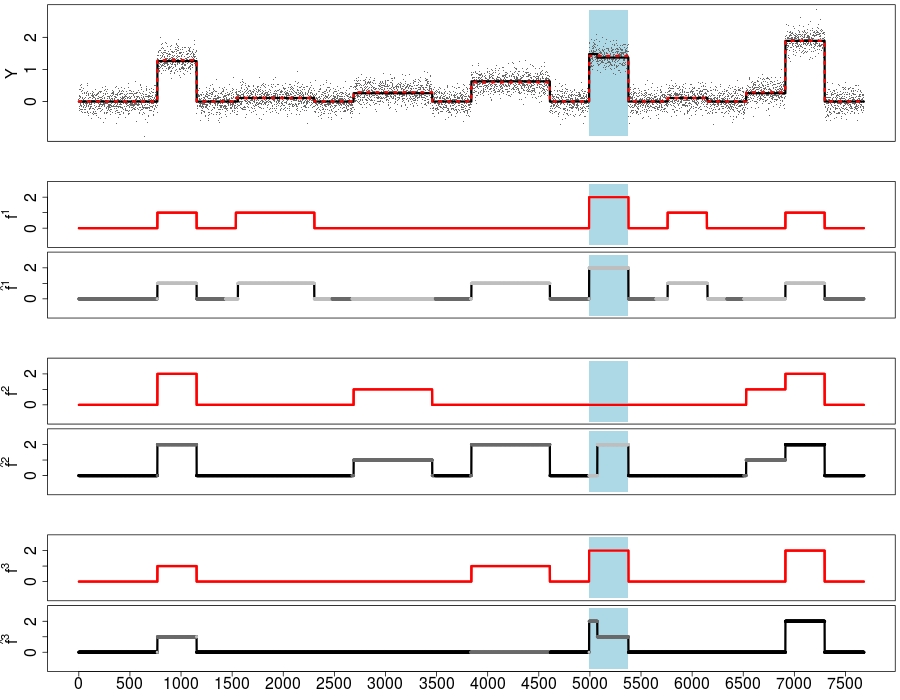
Fig 1.4: First row: gg (red dotted line), g^\hat{g} (black line) with ω^=(0.11,0.26,0.63)⊤\hat{\omega}=(0.11,0.26,0.63)^{\top}, and data YY (gray) from Example 1.1. Subsequent rows: fif^{i} (red line) and SLAM’s estimate f^i\hat{f}^{i} (gray/black line) for qn​(α)=0.2q_{n}(\alpha)=0.2 and qn​(β)=2.1q_{n}(\beta)=2.1 (see Section 4.6). Gray shades for segments of f^i\hat{f}^{i} indicate the confidence for the given segment: a maximal deviation of two (light gray), one (gray), and no deviation (black) at confidence level β=0.01\beta=0.01. The blue area displays a constant region of gg where g^\hat{g} includes a (wrong) jump and its effect on estimation of the sources.

Choosing α=αn\alpha=\alpha_{n} and β=βn\beta=\beta_{n} as in (23), in Section 2.4 (see Theorem 2.7) we show that with probability at least 1−αn1-\alpha_{n}, for nn large enough, the SLAM estimator f^\hat{f} in (25) estimates for all i=1,…,mi=1,\ldots,m

  1. 1.

    the respective number of c.p.’s K⁡(fi)K(f^{i}) correctly,

  2. 2.

    all c.p. locations with rate ln2⁡(n)/n\ln^{2}(n)/n simultaneously, and

  3. 3.

    the function values of fif^{i} exactly (up to the uncertainty in the c.p. locations).

Obviously, the rate in 2. is optimal up to possible log-factors as the sampling rate is 1/n1/n. From Theorem 2.7 it follows further (see Remark 2.9) that the minimax detection rates are even achieved (again up to possible log-factors) when δ,λ→0\delta,\lambda\to 0 (as n→∞n\to\infty).

Further, we will show that a slight modification ℋ~​(β)\tilde{\mathcal{H}}(\beta) of ℋ⁡(β)\mathcal{H}(\beta) in (26) constitutes an asymptotically uniform (for given ASB δ\delta and λ\lambda) multivariate confidence band for the source functions (f1,…,fm)(f^{1},\ldots,f^{m}) (see Section 2.3).

To illustrate, Figure 1.4 depicts SLAM’s estimates of the mixture g^=ω^⊤​f^\hat{g}=\hat{\omega}^{\top}\hat{f}, with ω^=(0.11,0.26,0.63)⊤\hat{\omega}=(0.11,0.26,0.63)^{\top}, and the source functions f^1\hat{f}^{1}, f^2\hat{f}^{2}, f^3\hat{f}^{3} from (25) with YY as in Example 1.1, β=0.01\beta=0.01 (corresponding to qn​(β)=2.1q_{n}(\beta)=2.1), and an automatic choice of α\alpha, the MVT-selection method explained in Section 4.6. In order to visualize ℋ~​(β)\tilde{\mathcal{H}}(\beta), we illustrate the provided confidence in gray scale encoding the projections of ℋ~​(β)\tilde{\mathcal{H}}(\beta) (recall the alphabet 𝔄={0,1,2}\mathfrak{A}=\{0,1,2\}).

1.5 Algorithms and software

SLAM’s estimate for ω\omega (see (21) and Algorithm CRW, in Section S2.1 in the supplement) can be computed with polynomial complexity between 𝒪⁡(nm)\mathcal{O}(n^{m}) and 𝒪⁡(n2​m)\mathcal{O}(n^{2m}) (see Section 3). Using dynamic programming, the final estimate of sources can then be computed with a complexity ranging from 𝒪⁡(n)\mathcal{O}(n) and 𝒪⁡(n2)\mathcal{O}(n^{2}) depending on the final solution (see Section 3 for details). An R-package including an implementation of SLAM is available on request.

1.6 Simulations

The performance of SLAM is investigated in a simulation study in Section 4. We first investigate accuracy of ω^\hat{\omega} and the confidence region 𝒞1−α​(Y)\mathcal{C}_{1-\alpha}(Y) as in (21) and (20). We found always higher coverage of 𝒞1−α​(Y)\mathcal{C}_{1-\alpha}(Y) than the nominal confidence level 1−α1-\alpha. In line with this, ω^\hat{\omega} appeared to be very stable under the choice of the confidence level α\alpha. Second, we investigate SLAM’s estimates f^\hat{f}. A major conclusion is that if gg is not well estimated in a certain region, this typically will influence the quality of the estimates of fif^{i} in this region but not beyond (see the marked lightblue region in Figure 1.4 where the estimator g^\hat{g} includes a wrong jump in a constant region of gg but this error does not propagate serially). This may be explained by the flexible c.p. model ℳδ\mathcal{M}^{\delta} together with the multiscale nature of SLAM, which locally ”repairs” estimation errors. Finally, in Section 4.6 we comment on practical choices for α\alpha and β\beta complementing the theoretically motivated choices in (23). To this end, we suggest a data driven selection method for α\alpha when it is considered as tuning parameter for the accuracy of the estimate ω^\hat{\omega} and f^\hat{f} rather than a confidence level for the coverage of ω\omega.

1.7 Application to cancer genetics

Blind source separation in the context of the SBSSR-model occurs in different areas, for example in digital communications and signal transmission. The main motivation for our work comes from cancer genetics, in particular from the problem to assign copy-number aberrations (CNAs) in cell samples taken from tumors (see [47]) to its clones. CNAs refer to stretches of DNA in the genomes of cancer cells which are under copy-number variation involving deletion or duplication of stretches of DNA relative to the inherited (germline) state present in normal tissues. CNAs are known to be key drivers of tumor progression through the deletion of “tumor suppressing” genes and the duplication of genes involved in processes such as cell signaling and division. Understanding where, when and how CNAs occur during tumourgenesis, and their consequences, is a highly active and important area of cancer research (see e.g., [7]). Modern high-throughput technologies allow for routine whole genome DNA sequencing of cancer samples and major international efforts are underway to characterize the genetic make up of all cancers, for example The Cancer Genome Atlas, http://cancergenome.nih.gov/.

A key component of complexity in cancer genetics is the “clonal” structure of many tumors, which relates to the fact that tumors usually contain distinct cell populations of genetic sub-types (clones) each with a distinct CNA profile (see e.g., [35, 60]). High-throughput sequencing technologies act by bulk measurement of large numbers of pooled cells in a single sample, extracted by a micro-dissection biopsy or blood sample for haematological cancers.

The copy-number, that is, number of copies of DNA stretches at a certain locus, of a single clone’s genome is a step function mapping chromosomal loci to a value i∈{0,…,k}i\in\{0,\ldots,k\} corresponding to ii copies of DNA at a locus, with reasonable biological knowledge of kk (in our example k=5k=5, see Section 5).

From the linear properties of the measurement technologies the relative amount of DNA measured at any loci is therefore a mixture of step functions, with mixture weights given by the relative proportion of the clone’s DNA in the pool. The estimation of the mixed function, that is, estimating the locations of varying overall copy numbers, has perceived considerable interest in the past (see [51, 73, 68, 40, 14, 50, 31, 26]). However, the corresponding demixing problem, that is, jointly estimating the number of clones, their proportion, and their CNAs, has only perceived more recently as an important issue and hence received very little attention in a statistical content so far and is the main motivation for this work.

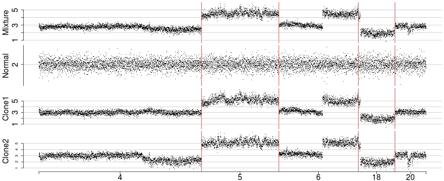
In Section 5, we illustrate SLAM’s ability to recover the CNA’s of such clones by utilizing it on real genetic sequencing data. On hand of a special data set, with measurements not only for the mixture but also for the underlying source functions (clones) and with knowledge about the mixing weights, we are able to report on the accuracy of SLAM’s estimates of the corresponding CNA profile and the mixing proportion of the clones.

1.8 Related work

Each, BSS of finite alphabet sources (see, e.g., [53, 44, 9, 72, 21, 46, 42, 36, 58]) and the estimation of step functions, with unknown number and location of c.p.’s (see, e.g., [12, 51, 30, 32, 68, 65, 40, 41, 74, 50, 61, 31, 48, 33, 39, 26]), are widely discussed problems. However, the combination of both, as discussed in this paper, is not. Rigorous statistical methodology and theory for finite alphabet BSS problems is entirely lacking to best of our knowledge and we are not aware of any other method which provides estimates for and confidence statements in the SBSSR-model in such a rigorous and general way. There are, however, related problems, discussed in the following.

Rewriting the SBSSR-model (4) in matrix form Y=F​ω+ϵY=F\omega+\epsilon with F=(fi​(xj))1≤j≤n,1≤i≤mF=(f^{i}(x_{j}))_{1\leq j\leq n,1\leq i\leq m} shows some commonality to signal recovery in linear models. In fact, our Theorem 1.3 reveals some analogy to exact and stable recovery results in compressive sensing and related problems (see [24, 11]). We stress, however, that there are fundamental differences. There typically the systems matrix FF is known and ω\omega is a sparse vector to be recovered, having only a very few non null coefficients. Under an additional finite alphabet assumption (for known FF) recovery of ω\omega is, for example, addressed in [25, 17, 8, 1]. In our setting both, FF and ω\omega are unknown.

Another related problem is non-negative matrix factorization (NMF) (see e.g., [43, 23, 2, 56]), where one assumes a multivariate signal Y∈ℝn×MY\in\mathds{R}^{n\times M} resulting from MM different (unknown) mixing vectors, that is, ω∈ℝ+m×M\omega\in\mathds{R}_{+}^{m\times M}, and an (unknown) non-negative source matrix F∈ℝ+n×mF\in\mathds{R}_{+}^{n\times m}. There, a fundamental assumption is that m≪min⁡(n,M)m\ll\min(n,M), which obviously does not hold in our case where M=1M=1. Instead we employ the additional assumption of a known finite alphabet, i.e., F∈𝔄n×mF\in\mathfrak{A}^{n\times m}. Indeed, techniques and algorithms for NMF are quite different from the ones derived here, as our methodology explicitly takes advantage of the one dimensional (i.e., ordered) c.p. structure under the finite alphabet assumption.

However, the identifiability conditions (6) and (7) from Section 1.2 are similar in nature to identifiability conditions for the NMF problem [23, 2], from where the notation “separable” originates. In order to ensure identifiability in the NMF problem, the “α\alpha-robust simplicial” condition (see e.g., [56, Definition 2.1]) on the mixing matrix ω∈ℝ+m×M\omega\in\mathds{R}_{+}^{m\times M} and the “separability” condition (see e.g. [56, Definition 2.2]) on the source matrix F∈ℝ+n×mF\in\mathds{R}_{+}^{n\times m} are well established [23, 2, 56].

There, the “α\alpha-robust simplicial” condition assumes that the mixing vectors ω1⋅,…,ωm⋅∈ℝM+\omega_{1\cdot},\ldots,\omega_{m\cdot}\in\mathds{R}^{M}_{+} constitute vertices of an mm-simplex with minimal diameter (distance between any vertex and the convex hull of the remaining vertices) α\alpha. This means that different source values Fi⋅∈ℝmF_{i\cdot}\in\mathds{R}^{m} are mapped to different mixture values Fi⋅ω∈ℝ+MF_{i\cdot}\omega\in\mathds{R}_{+}^{M} by the mixing matrix ω∈ℝ+m×M\omega\in\mathds{R}_{+}^{m\times M}. This condition is analog to the condition A​S​B​(ω)≥δASB(\omega)\geq\delta in (6), which also ensures that different source values f⁡(x)∈𝔄mf(x)\in\mathfrak{A}^{m} are mapped to different mixture values ω⊤​f​(x)∈ℝ\omega^{\top}f(x)\in\mathds{R} via the mixing weights ω∈Ω⁡(m)\omega\in\Omega(m), with minimal distance δ\delta between different mixture values.

The “separability” condition in NMF is the same as in Definition 1.2 but with AA replaced by the identitiy matrix (recall that in NMF the sources can take any positive value in ℝ+\mathds{R}_{+}, in contrast to the SBSSR-model where the sources can only take values in a given alphabet 𝔄\mathfrak{A}) and the intervals Ir⊂(0,1]I_{r}\subset(0,1] are replaced by measurement points ir∈{1,…,n}i_{r}\in\{1,\ldots,n\} (recall that the SBSSR-model considers a change-point regression setting, in contrast to NMF where observations do not necessarily come from discrete measurements of an underlying regression function). In both models (NMF and SBSSR) the separability condition ensures a certain variability of the sources in order to guarantee identitfiability of the mixing matrix and vector, respectively, from their mixture.

Besides NMF, there are many other matrix-factorization problems, which aim to decompose a multivariate signal Y∈ℝn×MY\in\mathds{R}^{n\times M} in two matrices of dimension n×mn\times m and m×Mm\times M, respectively. A popular example is independent component analysis (ICA) (see e.g., [16, 6, 3]), which exploits statistical independence of the mm different sources. We stress that this approach becomes infeasible in our setting where M=1M=1 as the error terms then sum up to a single error term and ICA would treat this as one observation. Other matrix-factorization methods assume a certain sparsity of the mixing-matrix [64]. Similar to NMF methods, in general all these methods, however, again rely on the assumption that M>1M>1 (most of them even require M≥mM\geq m) as otherwise the signal is not even identifiable, in contrast to our situation again due to the finite alphabet.

Minimization of the ℓ0\ell_{0} norm using dynamic programming (which has a long history in c.p. analysis, see e.g., [4, 30, 32, 41]) for segment estimation under a multiscale constraint has been introduced in [10] (see also [18] and [31]) and here we extend this to mixtures of segment signals and in particular to a finite alphabet restriction.

The SBSSR problem becomes tractable as we assume that our signals occur with sufficiently many alphabet combinations which may be present already on small scales on the one hand, and on the other hand we also observe long enough segments (large scales) in order to estimate reliably the corresponding mixing weights on these (see the identifiability condition in (7)). Both assumptions seem to be satisfied in our motivating application, the separation of clonal copy numbers in a tumor.

To best of our knowledge, the way we treat the problem of clonal separation is new, see, however, [71, 13, 47, 59, 37, 22]. Methods suggested there, all rely on specific prior information about the sources ff and cannot be applied to the general SBSSR-model. Moreover, most of them treat the problem from a Bayesian perspective.

2 Method and theory

2.1 Confidence region for the weights

Let YY and g=ω⊤​f∈ℳδg=\omega^{\top}f\in\mathcal{M}^{\delta} be as in the SBSSR-model (4). Our starting point for the recovery of the weights ω\omega and the sources ff is the construction of proper confidence sets for ω\omega which is also of statistical relevance by its own as the source functions are unknown which hinders direct inversion of a confidence set for gg.

Consider the system of boxes 𝔅={B⁡(i,j):1≤i≤j≤n}\mathfrak{B}=\{B(i,j):1\leq i\leq j\leq n\} from (16) with q=qn​(α)q=q_{n}(\alpha) as in (17) for some given α∈(0,1)\alpha\in(0,1), as described in Section 1.4.1.

As the underlying sources ff are assumed to be separable (see Definition 1.2 and (9)) there exist intervals [xir⋆,xjr⋆]⊂(0,1][x_{i^{\star}_{r}},x_{j^{\star}_{r}}]\subset(0,1], for r=1,…,mr=1,\ldots,m, such that

f|[xir⋆,xjr⋆]≡[A]r,f|_{[x_{i^{\star}_{r}},x_{j^{\star}_{r}}]}\equiv[A]_{r}, (27)

with AA as in (8). Assume for the moment that these intervals would be known and let B⋆:⁣=B(i1⋆,j1⋆)×…×B(im⋆,jm⋆)∈𝔅mB^{\star}\mathrel{\mathop{:}\!\!=}B(i^{\star}_{1},j^{\star}_{1})\times\ldots\times B(i^{\star}_{m},j^{\star}_{m})\in\mathfrak{B}^{m} be the corresponding mm-box. Then a 1−α1-\alpha confidence region for ω\omega is given as

𝒞1−α(i1⋆,j1⋆,…,im⋆,jm⋆):⁣=A−1B⋆.\mathcal{C}_{1-\alpha}(i^{\star}_{1},j^{\star}_{1},...,i^{\star}_{m},j^{\star}_{m})\mathrel{\mathop{:}\!\!=}A^{-1}B^{\star}. (28)

To see that (28) is, indeed, a 1−α1-\alpha confidence region for ω\omega, note that

{ω∈𝒞1−α(i1⋆,j1⋆,…,im⋆,jm⋆)}⊃⋂1≤r≤m{g|[xir⋆,xjr⋆]≡ω⊤[A]r∈B(ir⋆,jr⋆)}\{\omega\in\mathcal{C}_{1-\alpha}(i^{\star}_{1},j^{\star}_{1},...,i^{\star}_{m},j^{\star}_{m})\}\supset\bigcap_{1\leq r\leq m}\{g|_{[x_{i^{\star}_{r}},x_{j^{\star}_{r}}]}\equiv\omega^{\top}[A]_{r}\in B(i^{\star}_{r},j^{\star}_{r})\}

and

{Tn(Y,g)≤qn(α)}=⋂1≤i≤j≤ng|[xi,xj]≡gi​j{gi​j∈B(i,j)}.\{T_{n}(Y,g)\leq q_{n}(\alpha)\}=\bigcap_{\begin{subarray}{c}1\leq i\leq j\leq n\\ g|_{[x_{i},x_{j}]}\equiv g_{ij}\end{subarray}}\{g_{ij}\in B(i,j)\}.

This implies that

{ω∈𝒞1−α(i1⋆,j1⋆,…,im⋆,jm⋆)}⊃{Tn(Y,g)≤qn(α)}\{\omega\in\mathcal{C}_{1-\alpha}(i^{\star}_{1},j^{\star}_{1},...,i^{\star}_{m},j^{\star}_{m})\}\supset\{T_{n}(Y,g)\leq q_{n}(\alpha)\} (29)

and therefore it holds uniformly in g∈ℳδg\in\mathcal{M}^{\delta} that

P​(ω∈𝒞1−α​(i1⋆,j1⋆,…,im⋆,jm⋆))≥P​(Tn​(Y,g)≤qn​(α))≥1−α.\textbf{P}(\omega\in\mathcal{C}_{1-\alpha}(i^{\star}_{1},j^{\star}_{1},...,i^{\star}_{m},j^{\star}_{m}))\geq\textbf{P}(T_{n}(Y,g)\leq q_{n}(\alpha))\geq 1-\alpha. (30)

Of course, as the source functions ff are unknown, intervals [xir⋆,xjr⋆][x_{i^{\star}_{r}},x_{j^{\star}_{r}}] which satisfy (27) are not available immediately and thus, one cannot construct the mm-box B⋆B^{\star} required for (28) directly.

For this reason, we will describe a strategy to obtain a sub-system of mm-boxes, that is, a subset 𝔅⋆⊂𝔅m\mathfrak{B}^{\star}\subset\mathfrak{B}^{m}, which covers B⋆B^{\star} conditioned on {Tn(Y,g)≤qn(α)}\{T_{n}(Y,g)\leq q_{n}(\alpha)\} almost surely. To this end, observe that for any random set 𝒞⋆​(Y)⊂ℝm\mathcal{C}^{\star}(Y)\subset\mathds{R}^{m} with

P​(𝒞⋆​(Y)⊃𝒞1−α​(i1⋆,j1⋆,…,im⋆,jm⋆)|Tn​(Y,g)≤qn​(α))=1\textbf{P}\left(\mathcal{C}^{\star}(Y)\supset\mathcal{C}_{1-\alpha}(i^{\star}_{1},j^{\star}_{1},\ldots,i^{\star}_{m},j^{\star}_{m})\middle|T_{n}(Y,g)\leq q_{n}(\alpha)\right)=1 (31)

(29) and (30) imply P​(ω∈𝒞⋆​(Y))≥1−α\textbf{P}(\omega\in\mathcal{C}^{\star}(Y))\geq 1-\alpha. We then define 𝒞1−α\mathcal{C}_{1-\alpha} as in (20). To this end, 𝔅⋆\mathfrak{B}^{\star} is constructed such that the diameter of the resulting 𝒞1−α\mathcal{C}_{1-\alpha} is of order ln⁡(n)/n\ln(n)/\sqrt{n} (see Corollary 2.8). The construction will be done explicitly by an algorithm which relies on the application of certain reduction rules to 𝔅m\mathfrak{B}^{m} to be described in the following.

Let projr:𝔅m→𝔅\operatorname{proj}_{r}:\;\mathfrak{B}^{m}\;\rightarrow\;\mathfrak{B}, for r=1,…,mr=1,\ldots,m, denote the rr-th projection (i.e., projr(B1×…×Bm):⁣=Br\operatorname{proj}_{r}(B_{1}\times\ldots\times B_{m})\mathrel{\mathop{:}\!\!=}B_{r}) and define the set of boxes on which any signal fulfilling the multiscale constraint is non constant (nc) as

𝔅nc:⁣={B(i,j)∈𝔅:∃[s,t],[u,v]⊂[i,j] with B(s,t)∩B(u,v)=∅}.\mathfrak{B}_{\text{nc}}\mathrel{\mathop{:}\!\!=}\{B(i,j)\in\mathfrak{B}:\exists[s,t],[u,v]\subset[i,j]\text{ with }B(s,t)\cap B(u,v)=\emptyset\}. (32)
  • R 1.

    Delete B∈𝔅mB\in\mathfrak{B}^{m} if there exists an r∈{1,…,m}r\in\{1,\ldots,m\} such that B(i,j):⁣=projr(B)∈𝔅ncB(i,j)\mathrel{\mathop{:}\!\!=}\operatorname{proj}_{r}(B)\in\mathfrak{B}_{\text{nc}} as in (32).

The reasoning behind RR 1. is as follows. g|[xir⋆,xjr⋆]g|_{[x_{i_{r}^{\star}},x_{j_{r}^{\star}}]} is constant for r=1,…,mr=1,\ldots,m as f1,…,fmf^{1},\ldots,f^{m} are constant on [xir⋆,xjr⋆][x_{i_{r}^{\star}},x_{j_{r}^{\star}}]. Consequently, all mm-boxes that include a box B⁡(i,j)∈𝔅B(i,j)\in\mathfrak{B} such that gg cannot be constant on [xi,xj][x_{i},x_{j}] (conditioned on Tn​(Y,g)≤qn​(α)T_{n}(Y,g)\leq q_{n}(\alpha)) can be deleted in order to preserve coverage of B⋆B^{\star}. Let [xi,xj][x_{i},x_{j}] be an interval on which gg is constant (say g|[xi,xj]≡cg|_{[x_{i},x_{j}]}\equiv c) and assume that there exist intervals [s,t],[u,v]⊂[i,j][s,t],[u,v]\subset[i,j] such that B⁡(s,t)∩B⁡(u,v)=∅B(s,t)\cap B(u,v)=\emptyset. Then by construction of the boxes B⁡(s,t)B(s,t) and B⁡(u,v)B(u,v), Tn​(Y,g)≤qn​(α)T_{n}(Y,g)\leq q_{n}(\alpha) implies that c∈B⁡(s,t)c\in B(s,t) and c∈B⁡(u,v)c\in B(u,v), which contradicts B⁡(s,t)∩B⁡(u,v)=∅B(s,t)\cap B(u,v)=\emptyset. In other words, 𝔅nc\mathfrak{B}_{\text{nc}} (nc =^\hat{=} non constant ) in (32) includes all boxes B⁡(i,j)B(i,j) such that all function g~∈ℳδ\tilde{g}\in\mathcal{M}^{\delta} which fulfill the multiscale constraint Tn​(Y,g~)≤qn​(α)T_{n}(Y,\tilde{g})\leq q_{n}(\alpha) cannot be constant on [xi,xj][x_{i},x_{j}]. Note that, in contrast to the following two reduction rules, the reduction rule RR 1. does not depend on the specific matrix AA in the identifiablity condition in (7).

  • R 2.

    Delete B∈𝔅mB\in\mathfrak{B}^{m}, with [b¯r,b¯r]:⁣=projr(B)[\underline{b}_{r},\overline{b}_{r}]\mathrel{\mathop{:}\!\!=}\operatorname{proj}_{r}(B) if at least one of the following statements holds true

    1. 1.

      b¯1≤a1\overline{b}_{1}\leq a_{1} or b¯1≥a1+a2−a1m\underline{b}_{1}\geq a_{1}+\frac{a_{2}-a_{1}}{m},

    2. 2.

      for any 2≤r≤m2\leq r\leq m

      a2+(m−1)​a1−∑j=1r−1b¯jm−r+1≤b¯rorb¯r−1≥b¯r,\frac{a_{2}+(m-1)a_{1}-\sum_{j=1}^{r-1}\underline{b}_{j}}{m-r+1}\leq\underline{b}_{r}\quad\text{or}\quad\underline{b}_{r-1}\geq\overline{b}_{r},
    3. 3.

      ∑j=1mb¯j≤a2+(m−1)​a1\sum_{j=1}^{m}\overline{b}_{j}\leq a_{2}+(m-1)a_{1}.

RR 2. 1. comes from the fact that 0<ω1<1/m0<\omega_{1}<1/m, RR 2. 2. from ωi−1<ωi<(1−∑j=1i−1ωj)/(m−i+1)\omega_{i-1}<\omega_{i}<(1-\sum_{j=1}^{i-1}\omega_{j})/(m-i+1), and RR 2. 3. from ∑j=1mωj=1\sum_{j=1}^{m}\omega_{j}=1, together with the specific choice of the matrix AA in (8). For a different choice of AA in (7) the equations in RR 2. can be modified accordingly.

In what follows, define for k=1,…,nk=1,\ldots,n

𝒥k:⁣={[i,j]:k∈[i,j] and B(i,j)∉𝔅nc}.\mathcal{J}_{k}\mathrel{\mathop{:}\!\!=}\{[i,j]:k\in[i,j]\text{ and }B(i,j)\not\in\mathfrak{B}_{\text{nc}}\}. (33)
  • R 3.

    Delete B∈𝔅mB\in\mathfrak{B}^{m}, if there exists a k∈{1,…,n}k\in\{1,\ldots,n\} such that for all [i,j]∈𝒥k[i,j]\in\mathcal{J}_{k}

    [maxi≤u≤v≤j⁡b¯u​v,mini≤u≤v≤j⁡b¯u​v]∩{ω~⊤​a:a∈𝔄m​ and ​ω~∈A−1​B}\Big[\max_{i\leq u\leq v\leq j}\underline{b}_{uv},\min_{i\leq u\leq v\leq j}\overline{b}_{uv}\Big]\cap\Big\{\tilde{\omega}^{\top}a:a\in\mathfrak{A}^{m}\ \text{ and }\tilde{\omega}\in A^{-1}B\Big\} (34)

    is empty, with [b¯u​v,b¯u​v]:⁣=B(u,v)∈𝔅[\underline{b}_{uv},\overline{b}_{uv}]\mathrel{\mathop{:}\!\!=}B(u,v)\in\mathfrak{B}.

Conditioning on Tn​(Y,g)≤qn​(α)T_{n}(Y,g)\leq q_{n}(\alpha) implies ω∈A−1​B⋆\omega\in A^{-1}B^{\star}, and, in particular, that there exists an ω~∈A−1​B⋆\tilde{\omega}\in A^{-1}B^{\star} such that Im(g):⁣={g(x1),…,g(xn)}⊂{ω~⊤a:a∈𝔄m}.\operatorname{Im}(g)\mathrel{\mathop{:}\!\!=}\{g(x_{1}),\ldots,g(x_{n})\}\subset\{\tilde{\omega}^{\top}a:a\in\mathfrak{A}^{m}\}. Moreover, for every k∈{1,…,n}k\in\{1,\ldots,n\} there exists an interval [xi,xj][x_{i},x_{j}] where gg is constant with g|[xi,xj]≡g⁡(xk)∈Im⁡(g)g|_{[x_{i},x_{j}]}\equiv g(x_{k})\in\operatorname{Im}(g). So, Tn​(Y,g)≤qn​(α)T_{n}(Y,g)\leq q_{n}(\alpha) implies g⁡(xk)∈B⁡(u,v)g(x_{k})\in B(u,v) for all [u,v]⊂[i,j][u,v]\subset[i,j] and, therefore, for B=B⋆B=B^{\star} (34) is not empty (conditioned on Tn​(Y,g)≤qn​(α)T_{n}(Y,g)\leq q_{n}(\alpha)).

Remark 2.1 (Incorporating prior knowledge on minimal scales).
  1. a)

    If we restrict to a minimal scale λ∈(0,1)\lambda\in(0,1) on which a jump of gg may occur, that is, for τj\tau_{j}, j=0,…,K+1j=0,\ldots,K+1, being the c.p.’s of gg

    λ:⁣=minj∈{0,…,K}|τj+1−τj|>0,\lambda\mathrel{\mathop{:}\!\!=}\min_{j\in\{0,\ldots,K\}}\left|\tau_{j+1}-\tau_{j}\right|>0, (35)

    we can modify RR 3. with 𝒥k\mathcal{J}_{k} in (33) replaced by 𝒥k∩{[i,j]:j−i+1≥n​λ}\mathcal{J}_{k}\cap\{[i,j]:j-i+1\geq n\lambda\}.

  2. b)

    In many applications (see Section 5), it is very reasonable to assume apriori knowledge of a minimal interval length λ⋆\lambda^{\star} of [xir⋆,xjr⋆][x_{i_{r}^{\star}},x_{j_{r}^{\star}}] in (27). This means that there exists some interval Ir⊂[0,1)I_{r}\subset[0,1) of minimum size λ⋆\lambda^{\star}, where (f1,…,fm)(f^{1},\ldots,f^{m}) take the value [A]r[A]_{r} as in (8) for r=1,…,mr=1,\ldots,m. This is summarized in the following reduction rule.

    • R 4.

      Knowing that jr⋆−ir⋆+1≥λ⋆​nj^{\star}_{r}-i^{\star}_{r}+1\geq\lambda^{\star}n for r=1,…,mr=1,\ldots,m in (27), delete B∈𝔅mB\in\mathfrak{B}^{m} if there exists an r∈{1,…,m}r\in\{1,\ldots,m\} such that for B(i,j):⁣=projr(B)B(i,j)\mathrel{\mathop{:}\!\!=}\operatorname{proj}_{r}(B) j−i+1<λ⋆​nj-i+1<\lambda^{\star}n.

RR 1. - RR 4. is summarized in Algorithm CRW, in Section S2.1 in the supplement, for constructing a confidence region for ω\omega.

Remark 2.2 (Noninformative mm-box).

If 𝔅⋆=∅\mathfrak{B}^{\star}=\emptyset, we formally may set 𝒞1−α:⁣=Ω(m)\mathcal{C}_{1-\alpha}\mathrel{\mathop{:}\!\!=}\Omega(m), the trivial confidence region. As {𝔅⋆=∅}⊂{Tn(Y,g)>qn(α)}\{\mathfrak{B}^{\star}=\emptyset\}\subset\{T_{n}(Y,g)>q_{n}(\alpha)\}, the probability that this happens can be bounded from above by α\alpha. This is in general only a very rough bound, simulations show that 𝔅⋆=∅\mathfrak{B}^{\star}=\emptyset is hardly ever the case when α\alpha is reasonably small. For instance, in 10,00010,000 simulations of Example 1.1 with n=1280n=1280, σ=0.1\sigma=0.1, α=0.1\alpha=0.1 it did not happen once. Of course, when α↗1\alpha\nearrow 1, 𝔅⋆=∅\mathfrak{B}^{\star}=\emptyset finally, as no mixture g∈ℳδg\in\mathcal{M}^{\delta} can fulfill the multiscale constrained Tn​(Y,g)≤qT_{n}(Y,g)\leq q for arbitrarily small qq.

Remark 2.3 (Shape of 𝒞1−α\mathcal{C}_{1-\alpha}).

The previous construction of the confidence set 𝒞1−α\mathcal{C}_{1-\alpha} does not ensure that the confidence set is of mm-box form

[ω¯1,ω¯1]×…×[ω¯m,ω¯m].[\underline{\omega}_{1},\overline{\omega}_{1}]\times\ldots\times[\underline{\omega}_{m},\overline{\omega}_{m}]. (36)

In general it is a union of mm-boxes. However, we can always take the smallest covering mm-box of 𝒞1−α\mathcal{C}_{1-\alpha}, given by

[infω~∈𝒞1−αω~1,supω~∈𝒞1−αω~1]×…×[infω~∈𝒞1−αω~m,supω~∈𝒞1−αω~m],[\inf_{\tilde{\omega}\in\mathcal{C}_{1-\alpha}}\tilde{\omega}_{1},\sup_{\tilde{\omega}\in\mathcal{C}_{1-\alpha}}\tilde{\omega}_{1}]\times\ldots\times[\inf_{\tilde{\omega}\in\mathcal{C}_{1-\alpha}}\tilde{\omega}_{m},\sup_{\tilde{\omega}\in\mathcal{C}_{1-\alpha}}\tilde{\omega}_{m}], (37)

in order to get a confidence set as in (36). Note, that dist¯(ω,𝒞1−α)=⁣:d\overline{\operatorname{dist}}(\omega,\mathcal{C}_{1-\alpha})\mathrel{=\!\!\mathop{:}}d remains the same when we replace 𝒞1−α\mathcal{C}_{1-\alpha} by (37). To see this, consider 𝒞^:⁣=ω+[−d,d]m\hat{\mathcal{C}}\mathrel{\mathop{:}\!\!=}\omega+[-d,d]^{m}, which is a covering mm-box of 𝒞1−α\mathcal{C}_{1-\alpha}, so in particular 𝒞^\hat{\mathcal{C}} covers (37), with dist¯​(ω,𝒞^)=d\overline{\operatorname{dist}}(\omega,\hat{\mathcal{C}})=d.

Summing up, we have now constructed a confidence set 𝒞1−α\mathcal{C}_{1-\alpha} for the mixing vector ω\omega in the SBSSR-model. Given 𝒞1−α\mathcal{C}_{1-\alpha} SLAM estimates ω\omega as in (21). From this, in the next section we derive estimators for the sources f1,…,fmf^{1},\ldots,f^{m}.

2.2 Estimation of source functions

SLAM estimates f=(f1,…,fm)f=(f^{1},\ldots,f^{m}) by solving the constraint optimization problem (25), which admits a solution if and only if

minf~∈𝒮​(𝔄)m⁡Tn​(Y,ω^​(α)⊤​f~)≤qn​(β).\min_{\tilde{f}\in\mathcal{S}(\mathfrak{A})^{m}}T_{n}(Y,\hat{\omega}(\alpha)^{\top}\tilde{f})\leq q_{n}(\beta). (38)

(38) cannot be guaranteed in general but it can be shown that it holds asymptotically with probability one (see Theorem S1.1 in the supplement), independently of the specific choice of ω^∈𝒞1−α​(Y)\hat{\omega}\in\mathcal{C}_{1-\alpha}(Y) in (21). For finite nn our simulations show that violation of (38) is hardly ever the case. For instance, in 10,00010,000 simulation runs of Example 1.1 with α=β=0.1\alpha=\beta=0.1 it did not happen once. Therefore, in practice, failure of (38) might rather indicate that the model assumption is not correct (e.g., due to outliers) and could be treated by pre-processing of the data. Another strategy can be to decrease β\beta and hence the constraint in (38) as for β>β′\beta>\beta^{\prime} it holds that qn​(β′)>qn​(β)q_{n}(\beta^{\prime})>q_{n}(\beta).

Remark 2.4 (Incorporating identifiability conditions in SLAM).

The separability condition in (7) could be incorporated in the estimator (25), which provides a further restriction on ℋ⁡(β)\mathcal{H}(\beta) in (26). This may yield a finite sample improvement of SLAM, however, at the expense of being less robust if such a particular identifiability condition is violated (see Section 4.5.1 for a simulation study of SLAM when the identifiability conditions in (6) and (7) are violated).

2.3 Confidence bands for the source functions

Obviously, uniform confidence sets for ff cannot be obtained if we allow for an arbitrarily small distance between two c.p.’s of gg (as for any c.p. problem, see [31]). However, if we restrict to a minimal scale λ\lambda as in (35), the SLAM estimation procedure in (25) leads to asymptotically uniform confidence bands for the source functions f1,…,fmf^{1},\ldots,f^{m}. To this end, we introduce

ℳλδ:⁣={g∈ℳδ:minj∈{0,…,K⁡(g)}|τj+1−τj|≥λ},\mathcal{M}^{\delta}_{\lambda}\mathrel{\mathop{:}\!\!=}\Big\{g\in\mathcal{M}^{\delta}:\min_{j\in\{0,\ldots,K(g)\}}\left|\tau_{j+1}-\tau_{j}\right|\geq\lambda\Big\}, (39)

where, as in (1), τ0=0<τ1<…<τK⁡(g)<τK⁡(g)+1=1\tau_{0}=0<\tau_{1}<\ldots<\tau_{K(g)}<\tau_{K(g)+1}=1 denote c.p.’s of gg. Moreover, let T~n\tilde{T}_{n} be as in (14), but with p​e​n​(j−i+1)pen(j-i+1) replaced by p​e​n​(j−i+1)+((a2−a1)​ln⁡(n)/m+8​σ2​ln⁡(e/λ)/λ)​(j−i+1)/npen(j-i+1)+\left((a_{2}-a_{1})\ln(n)/m+\sqrt{8\sigma^{2}\ln(e/\lambda)/\lambda}\right)\sqrt{(j-i+1)/n} and let ℋ~​(β)\tilde{\mathcal{H}}(\beta) be as in (26) but with TnT_{n} replaced by T~n\tilde{T}_{n}. Then ℋ~​(β)\tilde{\mathcal{H}}(\beta) constitutes an asymptotically uniform confidence band as the following theorem shows.

Theorem 2.5.

Consider the SBSSR-model and let ω^\hat{\omega} be the SLAM estimator from (21) for α=αn\alpha=\alpha_{n} as in (23). Then, for ℋ~​(β)\tilde{\mathcal{H}}(\beta) as in (26) with TnT_{n} replaced by T~n\tilde{T}_{n}, ℋ~​(β)\tilde{\mathcal{H}}(\beta) provides an asymptotically uniform confidence region for the sources ff,

limn⟶∞infg∈ℳλδP​((f1,…,fm)∈ℋ~​(β))≥1−β.\lim_{n\longrightarrow\infty}\inf_{g\in\mathcal{M}^{\delta}_{\lambda}}\textbf{P}((f^{1},...,f^{m})\in\tilde{\mathcal{H}}(\beta))\geq 1-\beta.

For a proof see Section S1.3 in the supplement.

2.4 Consistency and rates

In the following, we investigate further theoretical properties of SLAM. As in Theorem 2.5 our results will be stated uniformly over the space ℳλδ\mathcal{M}^{\delta}_{\lambda} in (39), that is, for a given minimal length λ\lambda of the constant parts of the mixture gg and a given minimal ASB δ\delta as in (5). Define the constants

c1=δ2​(a2−a1)248600​σ2​m2​(ak−a1)2,c2=δ+2​σ2​ln⁡(e/λ)λ.c_{1}=\frac{\delta^{2}(a_{2}-a_{1})^{2}}{48600\sigma^{2}m^{2}(a_{k}-a_{1})^{2}},\quad c_{2}=\frac{\delta+\sqrt{2\sigma^{2}\ln(e/\lambda)}}{\sqrt{\lambda}}. (40)

Further, let N⋆∈ℕN^{\star}\in\mathds{N} be the smallest integer, s.t.

2​ln⁡(e​N⋆/ln2⁡(N⋆))ln2⁡(N⋆)+6​ln⁡(3​e/λ)N⋆​λ\displaystyle\sqrt{\frac{2\ln\left(eN^{\star}/\ln^{2}(N^{\star})\right)}{\ln^{2}(N^{\star})}}+\frac{\sqrt{6\ln(3e/\lambda)}}{\sqrt{N^{\star}\lambda}} ≤δ4​σ, and\displaystyle\leq\frac{\delta}{4\sigma},\quad\text{ and } (41)
ln⁡(N⋆)N⋆​λ\displaystyle\frac{\ln(N^{\star})}{\sqrt{N^{\star}\lambda}} ≤δ⁡(a2−a1)/(ak−a1)2​m​(δ+2​σ2​ln⁡(e/λ)).\displaystyle\leq\frac{\delta(a_{2}-a_{1})/(a_{k}-a_{1})}{2m(\delta+\sqrt{2\sigma^{2}\ln(e/\lambda)})}. (42)
Remark 2.6 (Behavior of N⋆N^{\star}).

Note that the left-hand side in (41) and (42) is decreasing in N⋆N^{\star}, respectively. For fixed λ\lambda and δ/σ↘0\delta/\sigma\searrow 0, (41) dominates the behavior of N⋆N^{\star} as it is essentially of the form σ/δ≤c⁡(λ)​ln⁡(N⋆)\sigma/\delta\leq c(\lambda)\sqrt{\ln(N^{\star})}, whereas (42) is of the form σ/δ≤c⁡(λ,𝔄,m)​N⋆/ln⁡(N⋆)\sigma/\delta\leq c(\lambda,\mathfrak{A},m)\sqrt{N^{\star}}/\ln(N^{\star}). Conversely, for fixed δ/σ\delta/\sigma and λ↘0\lambda\searrow 0, (42) dominates the behavior of N⋆N^{\star} as it is essentially of the form λ−1​ln⁡(λ−1)≤c⁡(δ/σ,𝔄,m)​N⋆/ln2⁡(N⋆)\lambda^{-1}\ln(\lambda^{-1})\leq c(\delta/\sigma,\mathfrak{A},m)N^{\star}/\ln^{2}(N^{\star}) whereas (41) is of the form λ−1​ln⁡(λ−1)≤c⁡(δ/σ)​N⋆\lambda^{-1}\ln(\lambda^{-1})\leq c(\delta/\sigma)N^{\star}.

Theorem 2.7.

Consider the SBSSR-model with g∈ℳλδg\in\mathcal{M}^{\delta}_{\lambda}. Let ω^\hat{\omega} and f^=(f^1,…,f^m)\hat{f}=(\hat{f}^{1},\ldots,\hat{f}^{m}) be the SLAM estimators from (21) and (25), respectively, with α=αn\alpha=\alpha_{n} and β=βn\beta=\beta_{n} as in (23). Further, let τ^i\hat{\tau}^{i} and τi\tau^{i} be the vectors of all c.p. locations of f^i\hat{f}^{i} and fif^{i}, respectively, for i=1,…,mi=1,\ldots,m. Then for all n>N⋆n>N^{\star} in (41) and (42) and for all i=1,…,mi=1,\ldots,m

  1. 1.

    K⁡(f^i)=K⁡(fi)K(\hat{f}^{i})=K(f^{i}) ,

  2. 2.

    maxj⁡|τ^ji−τji|≤2​ln2⁡(n)n\max_{j}|\hat{\tau}^{i}_{j}-\tau^{i}_{j}|\leq 2\frac{\ln^{2}(n)}{n},

  3. 3.

    maxj⁡|fi^|[τ^j,τ^j+1)−fi|[τj,τj+1)|=0\max_{j}\left|\hat{f^{i}}|_{[\hat{\tau}_{j},\hat{\tau}_{j+1})}-f^{i}|_{[\tau_{j},\tau_{j+1})}\right|=0, and

  4. 4.

    |ω^i−ωi|≤c2a2−a1​ln⁡(n)n\left|\hat{\omega}_{i}-\omega_{i}\right|\leq\frac{c_{2}}{a_{2}-a_{1}}\frac{\ln(n)}{\sqrt{n}}

with probability at least 1−exp⁡(−c1​ln2⁡(n))1-\exp(-c_{1}\ln^{2}(n)), with c1c_{1} and c2c_{2} as in (40).

From the proof of Theorem 2.7 (see Section S1.2 in the supplement) it also follows that assertions 1. - 4. hold for any ω^∈𝒞1−α​(Y)\hat{\omega}\in\mathcal{C}_{1-\alpha}(Y) and we obtain the following.

Corollary 2.8.

Consider the SBSSR-model with g∈ℳλδg\in\mathcal{M}^{\delta}_{\lambda}. Let 𝒞1−α​(Y)\mathcal{C}_{1-\alpha}(Y) be as in (20) and αn\alpha_{n} as in (23). Further, let dist¯\overline{\operatorname{dist}} be is as in (22). Then for all n>N⋆n>N^{\star} in (41) and (42)

dist¯​(ω,𝒞1−αn​(Y))<c2a2−a1​ln⁡(n)n\overline{\operatorname{dist}}(\omega,\mathcal{C}_{1-\alpha_{n}}(Y))<\frac{c_{2}}{a_{2}-a_{1}}\frac{\ln(n)}{\sqrt{n}}

with probability at least 1−exp⁡(−c1​ln2⁡(n))1-\exp(-c_{1}\ln^{2}(n)), with c1c_{1} and c2c_{2} as in (40).

Remark 2.9 (SLAM (almost) attains minimax rates).
  1. a)

    (C.p. locations) Theorem 2.7 states that we can recover the c.p. locations of fif^{i} in probability with rate ln2⁡(n)/n\ln^{2}(n)/n. Obviously, the estimation rate of the c.p. locations is bounded from below by the sampling rate 1/n1/n. Consequently, the rate of Theorem 2.7 differs from the optimal rate only by a ln2⁡(n)\ln^{2}(n) factor.

  2. b)

    (Weights) By the one-to-one correspondence between the weights and the function values of gg the weights’ detection rate ln⁡(n)/n\ln(n)/\sqrt{n} immediately follows from the box height in (16) with qn​(αn)∈𝒪⁡(ln⁡(n))q_{n}(\alpha_{n})\in\mathcal{O}(\ln(n)) and coincides with the optimal rate 𝒪⁡(1/n)\mathcal{O}(1/\sqrt{n}) up to a ln⁡(n)\ln(n) term.

  3. c)

    (Dependence on λ\lambda) The minimal scale λ\lambda in Theorem 2.7 may depend on nn, i.e., λ=λn\lambda=\lambda_{n}. In order to ensure consistency of SLAM’s estimates ω^\hat{\omega} and (f^1,…,f^m)(\hat{f}^{1},\ldots,\hat{f}^{m}), Theorem 2.7 requires that (41) and (42) holds (for a sufficiently large N⋆N^{\star}) and that c2​ln⁡(n)/n→0c_{2}\ln(n)/\sqrt{n}\rightarrow 0, as n→∞n\rightarrow\infty. By Remark 2.6 this is fulfilled whenever λ−1​ln⁡(λ−1)∈𝒪⁡(n/ln2⁡(n))\lambda^{-1}\ln(\lambda^{-1})\in\mbox{\scriptsize$\mathcal{O}$}(n/\ln^{2}(n)). This means that the statements 1. - 4. in Theorem 2.7 hold true asymptotically with probability one as the minimal scale λn\lambda_{n} of successive jumps in a sequence of mixtures gng_{n} does not asymptotically vanish as fast as of order ln3⁡(n)/n\ln^{3}(n)/n. We stress that no method can recover finer details of a bump signal (including the mixture gg) below its detection boundary which is of the order ln⁡(n)/n\ln(n)/n, that is, SLAM achieves this minimax detection rate up to a ln2⁡(n)\ln^{2}(n) factor (see [29, 31]).

  4. d)

    (Dependence on δ\delta) Just as the minimal scale λ\lambda, the minimal ASB δ\delta in Theorem 2.7 may depend on nn as well, that is, δ=δn\delta=\delta_{n}. Analog to c), the SLAM’s estimates remain consistent whenever δ−1∈𝒪⁡(ln⁡(n))\delta^{-1}\in\mbox{\scriptsize$\mathcal{O}$}\left(\sqrt{\ln(n)}\right), that is, the statements 1. - 4. in Theorem 2.7 hold true asymptotically with probability one if the minimal ASB δn\delta_{n} in a sequence of mixtures gng_{n} does not decrease as fast as of order 1/ln⁡(n)1/\sqrt{\ln(n)}. We stress that no method can recover smaller jump heights of the mixture gg below its minimax detection rate, which in 1/ln⁡(n)1/\ln(n). To see this, note that statement 2. in Theorem 2.7 provides asymptotic detection power one for 2​ln⁡(n)22\ln(n)^{2} i.i.d. observations with mean δn\delta_{n} (recall that the ASB corresponds to the minimal possible jump height of the mixture gg). Hence, SLAM achieves the minimax rate up to a ln⁡(n)\sqrt{\ln(n)} factor.

Remark 2.10 (SLAM for known ω\omega).

If ω\omega is known in the SBSSR-model, the second part of SLAM can be used separately. We may then directly solve (24) without pre-estimating ω\omega, that is, in Section 1.4.3, we simply replace ω^\hat{\omega} by ω\omega. Then, Theorem 2.5 is still valid for ℋ~​(β)\tilde{\mathcal{H}}(\beta) replaced by ℋ⁡(β)\mathcal{H}(\beta). Further, a careful modification of the proof of Theorem 2.7 shows that the assertions in Theorem 2.7 hold for a possibly smaller N⋆N^{\star} in (41) and (42) and for c1c_{1} replaced by 75​m2​(ak−a1)2​c1/(a2−a1)275m^{2}(a_{k}-a_{1})^{2}c_{1}/(a_{2}-a_{1})^{2}. We stress that the finite alphabet assumption is still required and the corresponding identifiability assumption A​S​B​(ω)≥δASB(\omega)\geq\delta must be valid.

3 Computational issues

SLAM is implemented in two steps. In the first step, for a given α∈(0,1)\alpha\in(0,1) a confidence region for the mixing weights ω\omega is computed as in Algorithm CRW (see Section 2.1 and S2.1). To this end, each of the n2​mn^{2m} mm-boxes in 𝔅m={B⁡(i,j):1≤i≤j≤n}m\mathfrak{B}^{m}=\{B(i,j):1\leq i\leq j\leq n\}^{m} needs to be examined with the reduction rules R1 - R4 for validity as a candidate box for the intervals [i1⋆,j1⋆]×…×[im⋆,jm⋆][i^{\star}_{1},j^{\star}_{1}]\times\ldots\times[i^{\star}_{m},j^{\star}_{m}], which yields the complexity 𝒪⁡(n2​m)\mathcal{O}(n^{2m}). There are, however, important pruning steps, which can lead to a considerably smaller complexity.

First, note that it suffices to consider mm-boxes which are maximal elements with respect to the partial order of inclusion, that is, for B1=[b¯11,b¯11]×…×[b¯m1,b¯m1]B^{1}=[\underline{b}_{1}^{1},\overline{b}_{1}^{1}]\times\ldots\times[\underline{b}_{m}^{1},\overline{b}_{m}^{1}], B2=[b¯12,b¯12]×…×[b¯m2,b¯m2]∈𝔅mB^{2}=[\underline{b}_{1}^{2},\overline{b}_{1}^{2}]\times\ldots\times[\underline{b}_{m}^{2},\overline{b}_{m}^{2}]\in\mathfrak{B}^{m}

B1≼B2⇔[b¯i1,b¯i1]⊆[b¯i2,b¯i2]for all ​i=1,…,m,B^{1}\preccurlyeq B^{2}\Leftrightarrow[\underline{b}_{i}^{1},\overline{b}_{i}^{1}]\subseteq[\underline{b}_{i}^{2},\overline{b}_{i}^{2}]\quad\text{for all }i=1,\ldots,m,

where an element aa of a partially ordered set PP is maximal if there is no element bb in PP such that b>ab>a. To see this, assume that an mm-box BB is not deleted by the reduction rule RR 3. in the second last line of Algorithm CRW, then an mm-box B′∈𝔅mB^{\prime}\in\mathfrak{B}^{m} with B′≺BB^{\prime}\prec B does not influence the confidence region 𝒞1−α\mathcal{C}_{1-\alpha} (see last line of Algorithm CRW), as A−1​B′⊂A−1​BA^{-1}B^{\prime}\subset A^{-1}B. Conversely, if an mm-box BB is deleted by the reduction rule RR 3. in the second last line of Algorithm CRW, then an mm-box B′∈𝔅mB^{\prime}\in\mathfrak{B}^{m} with B′≺BB^{\prime}\prec B will be deleted by RR 3. as well, such that B′B^{\prime} does not need to be considered either.

Second, note that the parameter ω\omega which is inferred in Algorithm CRW is global and hence, one can restrict to observations on a subinterval [xi,xj]⊂[0,1)[x_{i},x_{j}]\subset[0,1) as long as g|[xi,xj]g|_{[x_{i},x_{j}]} fulfills the identifiability conditions of ℳδ\mathcal{M}^{\delta}.

The explicit complexity of Algorithm CRW depends on the finial solution f^\hat{f} itself. Depending on the final f^\hat{f}, the above mentioned pruning steps yield a complexity between 𝒪⁡(nm)\mathcal{O}(n^{m}) and 𝒪⁡(n2​m)\mathcal{O}(n^{2m}). ω^\hat{\omega} is then computed as in (21).

In the second step, for a given β∈(0,1)\beta\in(0,1) and given ω^\hat{\omega} SLAM solves the constrained optimization problem (25), which can be done using dynamic programming. Frick et al. [31] provide a pruned dynamic programming algorithm to efficiently solve a one-dimensional version of (25) without the finite alphabet restriction in (73). As this restriction is crucial for SLAM we outline the details of the necessary modifications in Section S2.2 in the supplement. These modifications, however, do not change to complexity of the algorithm. Frick et al. [31] show that the overall complexity of the dynamic program depends on the final solution g^\hat{g} and is between 𝒪⁡(n)\mathcal{O}(n) and 𝒪⁡(n2)\mathcal{O}(n^{2}).

We stress finally that significant speed up (which is, however, not the subject of this paper) can be achieved by restricting the system of intervals in TnT_{n} and 𝔅\mathfrak{B}, respectively, to a smaller subsystem, for example, intervals of dyadic length, which for example reveals the complexity of the second step as 𝒪⁡(n​ln⁡(n))\mathcal{O}(n\ln(n)).

4 Simulations

In the following we investigate empirically the influence of all parameters and the underlying signal on the performance of the SLAM estimator. As performance measures we use the mean absolute error, MAE\operatorname{MAE}, for ω^\hat{\omega} and the mean absolute integrated error, MIAE\operatorname{MIAE}, for f^\hat{f}. Further, we report the centered mean, Mean⁡(K^)−K\operatorname{Mean}(\hat{K})-K, the centered median, Med⁡(K^)−K\operatorname{Med}(\hat{K})-K, of the number of c.p.’s of f^\hat{f}, the frequency of correctly estimated number of c.p.’s for the single source functions fif^{i}, Mean⁡(K^=K)i\operatorname{Mean}(\hat{K}=K)_{i}, and for the whole source function vector ff, Mean⁡(K^=K)\operatorname{Mean}(\hat{K}=K). To investigate the accuracy of the c.p. locations of the single estimated source functions f^1,…,f^m\hat{f}^{1},\ldots,\hat{f}^{m} we report the mean of maxi⁡minj​|τi−τ^j|\max_{i}\min_{j}\left|\tau_{i}-\hat{\tau}_{j}\right| and maxj⁡mini​|τi−τ^j|\max_{j}\min_{i}\left|\tau_{i}-\hat{\tau}_{j}\right|, where τ\tau and τ^\hat{\tau} denotes the vector of c.p. locations of the true signal and the estimate, respectively. Furthermore, we report common segmentation evaluation measures for the single estimated source functions f^1,…,f^m\hat{f}^{1},\ldots,\hat{f}^{m}, namely the entropy-based VV-measure, V1\operatorname{V_{1}}, with balancing parameter 11 of [57] and the false positive sensitive location error, FPSLE\operatorname{FPSLE}, and the false negative sensitive location error, FNSLE\operatorname{FNSLE}, of [34]. The VV-measure, taking values in [0,1][0,1], measures whether given clusters include the correct data points of the corresponding class. Larger values indicate higher accuracy, 11 corresponding to a perfect segmentation. The FPSLE\operatorname{FPSLE} and the FNSLE\operatorname{FNSLE} capture the average distance between true and estimated segmentation boundaries, with FPSLE being larger if a spurious split is included, while FNSLE getting larger if a true boundary is not detected (see [34] for details). To investigate the performance of the confidence region 𝒞1−α\mathcal{C}_{1-\alpha} for ω\omega, we use dist¯​(ω,𝒞1−α)\overline{\operatorname{dist}}(\omega,\mathcal{C}_{1-\alpha}) from (22), the mean coverage Mean⁡(ω∈𝒞1−α)\operatorname{Mean}(\omega\in\mathcal{C}_{1-\alpha}), and the diameters ω¯i−ω¯i\overline{\omega}_{i}-\underline{\omega}_{i}, where 𝒞1−α=[ω¯1,ω¯1]×…×[ω¯m,ω¯m]\mathcal{C}_{1-\alpha}=[\overline{\omega}_{1},\underline{\omega}_{1}]\times\ldots\times[\overline{\omega}_{m},\underline{\omega}_{m}]. Further, we report the mean coverage of the confidence band ℋ~​(β)\tilde{\mathcal{H}}(\beta), i.e. Mean⁡(f∈ℋ~​(β))\operatorname{Mean}(f\in\tilde{\mathcal{H}}(\beta)). In order to reduce computation time, we only considered intervals of dyadic length as explained in Section 3, possibly at expense of detection power. Simulation runs were always 10,00010,000.

4.1 Number of source functions mm

In order to illustrate the influence of the number of source functions mm on the performance of SLAM we vary m=2,…,5m=2,\ldots,5 while keeping the other parameters in the SBSSR- model fixed.

We investigate a binary alphabet 𝔄={0,1}\mathfrak{A}=\{0,1\} and set fi=𝟙[(i−1)/5,i/5)f^{i}=\mathds{1}_{[(i-1)/5,i/5)} for i=1,…,5i=1,\ldots,5, simple bump functions. For each m∈{2,3,4,5}m\in\{2,3,4,5\}, we choose ω\omega such that A​S​B​(ω)=0.02ASB(\omega)=0.02 in (5) (see Table S3.1 in the supplement). For σ=δ=0.02\sigma=\delta=0.02, n=1000n=1000, and α=β=0.1\alpha=\beta=0.1, we compute ω^\hat{\omega}, 𝒞0.9\mathcal{C}_{0.9}, f^1,…,f^m\hat{f}^{1},\ldots,\hat{f}^{m}, and ℋ~​(0.1)\tilde{\mathcal{H}}(0.1) for each m∈{2,3,4,5}m\in\{2,3,4,5\}, incorporating prior knowledge λ≥0.025\lambda\geq 0.025 (see (35) and Remark 2.1) (with truth λ=0.05\lambda=0.05). The results are displayed in Table S3.2. A major finding is that as the number of possible mixture values equals kmk^{m}, the complexity of the SBSSR-model grows exponentially in mm such that demixing becomes substantially more difficult with increasing mm.

4.2 Number of alphabet values kk

To illustrate the influence of the number of alphabet values kk, we consider three different alphabets 𝔄k={0,…,k}\mathfrak{A}_{k}=\{0,\ldots,k\} for k=2,3,4k=2,3,4. For m=2m=2, we set

f1=∑i=015(imodk)𝟙[i,i+1)/16,f2=∑i=0[15/k](imodk)𝟙k[i,i+1)/16,f^{1}=\sum_{i=0}^{15}\left(i\mod k\right)\mathds{1}_{[i,i+1)/16},\quad f^{2}=\sum_{i=0}^{[15/k]}\left(i\mod k\right)\mathds{1}_{k[i,i+1)/16}, (43)

step functions taking successively every alphabet value in 𝔄2\mathfrak{A}^{2} (see Figure S3.1 in the supplement). Further, we set ω=(0.02,0.98)\omega=(0.02,0.98) such that A​S​B​(ω)=0.02ASB(\omega)=0.02 for k=2,3,4k=2,3,4. For σ=0.05\sigma=0.05, n=1056n=1056, and α=β=0.1\alpha=\beta=0.1 we compute ω^\hat{\omega}, 𝒞0.9\mathcal{C}_{0.9}, f^1,…,f^m\hat{f}^{1},\ldots,\hat{f}^{m}, and ℋ~​(0.1)\tilde{\mathcal{H}}(0.1) for each k=2,3,4k=2,3,4, incorporating prior knowledge λ≥1/32\lambda\geq 1/32 (see (35) and Remark 2.1) (with truth λ=1/16\lambda=1/16). The results are displayed in Table S3.3 in the supplement. From this we find that an increasing kk does not influence SLAM’s performance for ω^\hat{\omega} and 𝒞1−α\mathcal{C}_{1-\alpha} too much. However, the model complexity kmk^{m} increases polynomially (for m=2m=2 as in Table S3.3 quadratically) in kk, reflected in a decrease of SLAM’s performance for the estimate of the source functions f^\hat{f}.

4.3 Confidence levels α\alpha and β\beta

We illustrate the influence of the confidence levels α\alpha and β\beta on SLAM’s performance with ff and ω\omega as in Example 1.1, that is, m=3m=3, 𝔄={0,1,2}\mathfrak{A}=\{0,1,2\}, ω=(0.11,0.29,0.6)\omega=(0.11,0.29,0.6), and ff as displayed in Figure 1.1. For σ=0.02,0.05,0.1\sigma=0.02,0.05,0.1 and n=1280n=1280, we compute ω^\hat{\omega}, 𝒞1−α\mathcal{C}_{1-\alpha}, f^1,…,f^m\hat{f}^{1},\ldots,\hat{f}^{m}, and ℋ~​(β)\tilde{\mathcal{H}}(\beta) for each (α,β)∈{0.01,0.05,0.1}2(\alpha,\beta)\in\{0.01,0.05,0.1\}^{2}, incorporating prior knowledge λ≥0.025\lambda\geq 0.025 (see (35) and Remark 2.1) (with truth λ=0.05\lambda=0.05). Results are displayed in Table S3.4 and Table S3.5 in the supplement. These illustrate that SLAM’s estimate ω^\hat{\omega} for the mixing weights is very stable under the choice of α\alpha. The diameters dist¯​(ω,𝒞1−α)\overline{\operatorname{dist}}(\omega,\mathcal{C}_{1-\alpha}) and ω¯i−ω¯i\overline{\omega}_{i}-\underline{\omega}_{i}, respectively decrease slightly with increasing α\alpha, as expected. Further, we found that the coverage Mean⁡(ω∈𝒞1−α)\operatorname{Mean}(\omega\in\mathcal{C}_{1-\alpha}) is always bigger than the nominal coverage 1−α1-\alpha indicating the conservative nature of the first inequality in (30). With increasing β\beta the multiscale constraint in (24) becomes stricter leading to an increase of K^\hat{K}. However, as Table S3.5 illustrates, this effect is remarkably small, resulting also in a high stability of f^\hat{f} with respect to α\alpha and β\beta. In contrast to the uniform coverage of the confidence region 𝒞1−α\mathcal{C}_{1-\alpha} for ω\omega for finite nn (recall (19)), this holds only asymptotically for the confidence band ℋ~​(β)\tilde{\mathcal{H}}(\beta) (see Theorem 2.5). This is reflected in Table S3.5, where with increasing σ\sigma the coverage Mean⁡(f∈ℋ~​(β))\operatorname{Mean}(f\in\tilde{\mathcal{H}}(\beta)) can be smaller than the nominal 1−β1-\beta. Nevertheless, the coverage of the single source functions remains reasonably high even for large σ\sigma (see Table S3.5). In summary, we draw from Table S3.4 and S3.5 a high stability of SLAM in the tuning parameters α\alpha and β\beta, for both, the estimation error and the confidence statements, respectively.

4.4 Prior information on the minimal scale λ\lambda

In the previous simulations we always included prior information on the minimal scale λ\lambda (see (35) and Remark 2.1). In the following, we demonstrate the influence of this prior information on SLAM’s performance in Example 1.1, that is, m=3m=3, 𝔄={0,1,2}\mathfrak{A}=\{0,1,2\}, ω=(0.11,0.29,0.6)\omega=(0.11,0.29,0.6), and ff as displayed in Figure 1.1. For σ=0.02\sigma=0.02, n=1280n=1280, and α=β=0.1\alpha=\beta=0.1 we compute ω^\hat{\omega}, 𝒞0.9\mathcal{C}_{0.9}, f^1,…,f^m\hat{f}^{1},\ldots,\hat{f}^{m}, and ℋ~​(0.1)\tilde{\mathcal{H}}(0.1) under prior knowledge λ≥\lambda\geq 0.050.05, 0.040.04, 0.0250.025, 0.0150.015, 0.0050.005 (with truth λ=0.05\lambda=0.05). The results in Table S3.9 in the supplement show a certain stability for a wide range of prior information on λ\lambda. Only when the prior assumptions on λ\lambda is of order 0.1​λ0.1\lambda (or smaller) SLAM’s performance gets significantly worse.

4.5 Robustness of SLAM

Finally, we want to analyze SLAM’s robustness against violations of model assumptions.

4.5.1 Robustness against non-identifiability

Throughout this work, we assumed g∈ℳδg\in\mathcal{M}^{\delta}, that is, ω∈Ωδ​(m)\omega\in\Omega^{\delta}(m) as in (6) and f∈𝒮​(𝔄)mf\in\mathcal{S}(\mathfrak{A})^{m} separable as in (7), in order to ensure identifiability. In the following, we briefly investigate SLAM’s behavior if these conditions are close to be, or even violated.

Alphabet separation boundary δ\delta

We start with the identifiability condition ω∈Ωδ​(m)\omega\in\Omega^{\delta}(m), i.e., A​S​B​(ω)≥δ>0ASB(\omega)\geq\delta>0 as in (5). We reconsider Example 1.1, that is, m=3m=3, 𝔄={0,1,2}\mathfrak{A}=\{0,1,2\}, and ff as displayed in Figure 1.1, but with ω\omega chosen randomly, uniformly distributed on Ω⁡(3)\Omega(3). For σ=0.05\sigma=0.05, n=1280n=1280, and α=β=0.1\alpha=\beta=0.1 we compute ω^\hat{\omega}, 𝒞1−α\mathcal{C}_{1-\alpha}, f^1,f^2,f^3\hat{f}^{1},\hat{f}^{2},\hat{f}^{3}, and ℋ~​(β)\tilde{\mathcal{H}}(\beta), incorporating prior knowledge λ≥0.025\lambda\geq 0.025 (see (35) and Remark 2.1) (with truth λ=0.05\lambda=0.05). Consequently, for each run we get a different ω\omega and A​S​B​(ω)ASB(\omega), respectively.

We found that SLAM’s performance of ω^\hat{\omega} and 𝒞1−α\mathcal{C}_{1-\alpha}, respectively, is not much influenced by A​S​B​(ω)ASB(\omega) (see Table S3.7, where the average mean squared error of ω^\hat{\omega} and dist¯​(ω,𝒞1−α)\overline{\operatorname{dist}}(\omega,\mathcal{C}_{1-\alpha}) remain stable when A​S​B​(ω)ASB(\omega) becomes small). The situation changes of course, when it comes to estimation of ff itself. A​S​B​(ω)=0ASB(\omega)=0 in (5) implies non-identifiability of ff, that is, it is not possible to recover ff uniquely. Therefore, it is expected that small A​S​B​(ω)ASB(\omega) will lead to a bad performance of any estimator of ff. This is also reflected in Theorem 2.7 where δ\delta, with A​S​B​(ω)≥δASB(\omega)\geq\delta, appears as a “conditioning number” of the SBSSR-problem. The results in Table S3.8 in the supplement confirm the strong influence of A​S​B​(ω)ASB(\omega) on the performance of SLAM’s estimate for ff. However, as SLAM does not only give an estimate of ff but also a confidence band ℋ~​(β)\tilde{\mathcal{H}}(\beta) this (unavoidable) uncertainty is also reflected in its coverage. To illustrate this define a local version of A​S​B​(ω)ASB(\omega) as ASBx(ω):⁣=mina≠f⁡(x)∈𝔄m|ω⊤a−ω⊤f(x)|ASB_{x}(\omega)\mathrel{\mathop{:}\!\!=}\min_{a\neq f(x)\in\mathfrak{A}^{m}}\left|\omega^{\top}a-\omega^{\top}f(x)\right|. Intuitively, A​S​Bx​(ω)ASB_{x}(\omega) determines the difficulty to discriminate between the source functions at a certain location x∈[0,1)x\in[0,1). Now, define the local size of ℋ~​(β)\tilde{\mathcal{H}}(\beta) as |ℋ~x(β)|:⁣=#{a∈𝔄m:∃f∈ℋ~(β) s.t. f(x)=a}|\tilde{\mathcal{H}}_{x}(\beta)|\mathrel{\mathop{:}\!\!=}\#\{a\in\mathfrak{A}^{m}:\exists f\in\tilde{\mathcal{H}}(\beta)\text{ s.t. }f(x)=a\}. Table S3.8 in the supplement shows that the uncertainty in |ℋ~x​(β)||\tilde{\mathcal{H}}_{x}(\beta)| increases in non-identifiable regions, that is, when A​S​Bx​(ω)ASB_{x}(\omega) is small.

Violation of separability condition

Next, we consider the separability condition in (7). We consider a modification of Example 1.1, that is, m=3m=3, 𝔄={0,1,2}\mathfrak{A}=\{0,1,2\}, where we modified the source function f1f^{1} in such a way, that it violates the separability condition in (7) for r=1r=1 (see Figure S3.2 in the supplement). For σ=0.05\sigma=0.05, n=1280n=1280, and α=β=0.1\alpha=\beta=0.1, we compute ω^\hat{\omega} and f^1,f^2,f^3\hat{f}^{1},\hat{f}^{2},\hat{f}^{3} incorporating prior knowledge λ≥0.025\lambda\geq 0.025 (see (35) and Remark 2.1) (with truth λ=0.05\lambda=0.05). The results are shown in Table S3.6 in the supplement. The violation of the separability condition in (7) leads to non-identifiabilty of ω\omega, which is naturally reflected in a worse performance of SLAM’s estimate of ω\omega. As the condition is violated for r=1r=1 this has a particular impact on ω^1\hat{\omega}_{1}. The performance for ω^2\hat{\omega}_{2} and ω^3\hat{\omega}_{3} remains relatively stable. The same holds true for f^\hat{f} itself, where the estimation error of ω^1\hat{\omega}_{1} propagates to a certain degree to the estimation of f^1\hat{f}^{1}. The performance of f^2\hat{f}^{2} and f^3\hat{f}^{3}, however, is not much influenced.

4.5.2 Violation of normality assumption

In the SBSSR-model we assume that the error distribution is normal, that is, ϵ=(ϵ1,…,ϵn)⊤∼𝒩⁡(0,In)\epsilon=(\epsilon_{1},\ldots,\epsilon_{n})^{\top}\sim\mathcal{N}(0,I_{n}). In the following we study SLAM’s performance for tt-(heavy tails) and χ2\chi^{2}-(skewed) distributed errors. Again, we reconsider Example 1.1, that is, m=3m=3, 𝔄={0,1,2}\mathfrak{A}=\{0,1,2\}, and ff as displayed in Figure 1.1. We add to gg now tt-distributed and χ2\chi^{2}-distributed errors, respectively, with 33 degrees of freedom, re-scaled to a standard deviation of σ=0.05\sigma=0.05. For n=1280n=1280 and α=0.1\alpha=0.1, we compute ω^\hat{\omega} and f^1,f^2,f^3\hat{f}^{1},\hat{f}^{2},\hat{f}^{3}, incorporating prior knowledge λ≥0.025\lambda\geq 0.025 (see (35) and Remark 2.1) (with truth λ=0.05\lambda=0.05). We simulated the statistic TnT_{n} for tt- and χ2\chi^{2}- distributed errors, respectively, and choose q⁡(β)q(\beta) to be the corresponding 90%90\% quantile. For tt-distributed errors this gave q⁡(β)=13.03q(\beta)=13.03 and for χ2\chi^{2}-distributed errors q⁡(β)=3.73q(\beta)=3.73. The results (see Table S3.6 in the supplement) indicate a certain robustness to misspecification of the error distribution, provided the quantiles for TnT_{n} are adjusted accordingly.

4.6 Selection of qn​(α)q_{n}(\alpha) and qn​(β)q_{n}(\beta)

On the one hand, for given α\alpha and β\beta SLAM yields confidence statements for the weights ω\omega and the source functions ff at level 1−α1-\alpha and 1−β1-\beta, respectively. This suggests the choice of these parameters as confidence levels. On the other hand, when we target to estimate ω\omega and ff qn​(α)q_{n}(\alpha) and qn​(β)q_{n}(\beta) can be seen as tuning parameters for the estimates ω^\hat{\omega} and f^\hat{f}. Although, we found in Section 4.3 that SLAM’s estimates are quite stable for a range of α\alpha’s and β\beta’s, a fine tuning of these parameters improves estimation accuracy, of course. In the following, we suggest a possible strategy for this. First, we discuss qn​(α)q_{n}(\alpha) for tuning the estimate ω^q:⁣=ω^(Y,q)\hat{\omega}_{q}\mathrel{\mathop{:}\!\!=}\hat{\omega}(Y,q) . Recall that for estimating ω\omega, qn​(β)q_{n}(\beta) is not required.

Minimal valid threshold (MVT)

Theorem 2.7 yields ln⁡(n)/n\ln(n)/\sqrt{n}-consistency of ω^\hat{\omega} when qn​(α)=qn​(αn)q_{n}(\alpha)=q_{n}(\alpha_{n}) with αn\alpha_{n} as in (23), independently of the specific choice of ω^∈𝒞1−αn\hat{\omega}\in\mathcal{C}_{1-\alpha_{n}}. Further, for α′\alpha^{\prime} (and qn​(α′)q_{n}(\alpha^{\prime}), respectively) with α′≥αn\alpha^{\prime}\geq\alpha_{n} (and qn​(α′)≤qn​(αn)q_{n}(\alpha^{\prime})\leq q_{n}(\alpha_{n}) , respectively) 𝒞1−α′⊆𝒞1−αn\mathcal{C}_{1-\alpha^{\prime}}\subseteq\mathcal{C}_{1-\alpha_{n}} whenever 𝔅⋆=𝔅qn​(α′)⋆≠∅\mathfrak{B}^{\star}=\mathfrak{B}^{\star}_{q_{n}(\alpha^{\prime})}\neq\emptyset in (20). Thus, choosing the threshold qq, for any discrete set Q={q1,q2,…,qN=qn​(αn)}Q=\{q_{1},q_{2},\ldots,q_{N}=q_{n}(\alpha_{n})\}, as q⋆:⁣=min(q∈Q:𝔅q⋆≠∅)q^{\star}\mathrel{\mathop{:}\!\!=}\min\left(q\in Q:\mathfrak{B}^{\star}_{q}\neq\emptyset\right) guarantees the convergence rates of Theorem 2.7 for the corresponding estimate ω^​(Y,q⋆)\hat{\omega}(Y,q^{\star}). In practice, we found Q={−1.0,−0.9,…,1.9,2.0}Q=\{-1.0,-0.9,...,1.9,2.0\} to be a sufficiently rich candidate set.

Sample splitting (SST)

Alternatively, we can choose qq such that a given performance measure h(q):⁣=E[L(ω^q−ω)]h(q)\mathrel{\mathop{:}\!\!=}\operatorname{E}[L(\hat{\omega}_{q}-\omega)] for estimating ω\omega, for example, the MSE with L=∥⋅∥22L=\|\cdot\|^{2}_{2}, is minimized. As ω\omega is unknown, we have to estimate h⁡(q)h(q), for which we suggest a simple sample splitting procedure. Details are given in Section S4, in the supplement. Simulations indicate that, especially for high noise level, the MVT-selection method outperforms the SST-selection method in terms of standard performance measures like MSE and MAE. However, in contrast to the SST-selection method, the MVT-selection method cannot be tailored for a specific performance measure hh.

It remains to select qn​(β)q_{n}(\beta) (and β\beta, respectively), which is required additionally for f^\hat{f}, recall (25) and (26). Theorem 2.7 suggests to choose qn​(β)=qn​(βn)q_{n}(\beta)=q_{n}(\beta_{n}) with βn\beta_{n} as in (23), i.e., qn​(β)→∞q_{n}(\beta)\rightarrow\infty with rate 𝒪⁡(log⁡(n))\mathcal{O}(\log(n)). For finite nn, there exist several methods for selection of qn​(β)q_{n}(\beta) in c.p. regression (see e.g., [73]), which might be used here as well. However, due to the high stability of f^\hat{f} in qq (see Section 4.3 and Figure S4.2 in the supplement) we simply suggest to choose β=0.1\beta=0.1, which we have used here for our data analysis. This choice controls the probability of overestimating the number of jumps in gg, P​(K⁡(g^)>K⁡(g))≤0.1\textbf{P}(K(\hat{g})>K(g))\leq 0.1 asymptotically. In general, it depends on the application. A large qn​(β)q_{n}(\beta) (hence small β\beta) has been selected in the subsequent application to remove spurious changes in the signal which appear biologically not as of much relevance.

5 Genetic sequencing data

Recall from Section 1.7 that a tumor often consists of a few distinct sub-populations , so called clones, of DNA with distinct copy-number profiles arising from duplication and deletion of genetic material groups. The copy number profiles of the underlying clones in a sample measurement correspond to the functions f1,…,fmf^{1},\ldots,f^{m}, the weights ω1,…,ωm\omega_{1},\ldots,\omega_{m} correspond to their proportion in the tumor, and the measurements correspond to the mixture gg with some additive noise.

The most common method for tumor DNA profiling is via whole genome sequencing, which roughly involves the following steps:

  1. 1.

    Tumor cells are isolated, and the pooled DNA is extracted, amplified and fragmented through shearing into single-strand pieces.

  2. 2.

    Sequencing of the single pieces takes place using short “reads” (at time of writing of around 10210^{2} base-pairs long).

  3. 3.

    Reads are aligned and mapped to a reference genome (or the patient germline genome if available) with the help of a computer.

Although, the observed total reads are discrete (each observation corresponds to an integer number of reads at a certain locus), for a sufficiently high sequencing coverage, as it is the case in our example with around 5555 average stretches of DNA mapped to a locus, it is well established to approximate this binomial by a normal variate (see [47] and references there).

In the following, SLAM is applied to the cell line LS411, which comes from colorectal cancer and a paired lymphoblastoid cell line. Sequencing was done through a collaboration of Complete Genomics with the Wellcome Trust Center for Human Genetics at the University of Oxford. This data has the special feature of being generated under a designed experiment using radiation of the cell line (“in vitro”), designed to produce CNAs that mimic real world copy-number events. In this case therefore, the mixing weights and sequencing data for the individual clones are known, allowing for validation of SLAM’s results, something that is not feasible for patient cancer samples.

The data comes from a mixture of three different types of DNA, relating to a normal (germline) DNA and two different clones. Tumor samples, even from micro-dissection, often contain high proportion of normal cells, which for our purposes are a nuisance, this is known as “stromal contamination” of germline genomes in the cancer literature. The true mixing weights in our sample are ω⊤=(ωNormal,ωClone1,ωClone2)=(0.2,0.35,0.45).\omega^{\top}=(\omega_{\text{Normal}},\omega_{\text{Clone1}},\omega_{\text{Clone2}})=(0.2,0.35,0.45).

SLAM will be, in the following, applied only to the mixture data without knowledge of ω\omega and the sequenced individual clones and germline. The latter (which serve as ground truth) will then be used only for validation of SLAM’s reconstruction. We restricted attention to regions of chromosome 4,5,6,184,5,6,18 and 2020, as detailed below. Figure S3.3 in the supplement shows the raw data. Sequencing produces some spatial artefacts in the data, and waviness related to the sequencing chemistry and local GC-content, corresponding to the relative frequency of the DNA bases {\{C, G}\} relative to {\{A, T}\}. This violates the modeling assumptions. To alleviate this we preprocess the data with a smoothing filter using local polynomial kernel regression on normal data, baseline correction, and binning. We used the local polynomial kernel estimator from the R package KernSmooth, with bandwidth chosen by visual inspection. We selected the chromosomal regions above as those showing reasonable denoising, and take the average of every 10th data point to make the computation manageable resulting in n=7480n=7480 data points spanning the genome. The resulting data is displayed in Figure S3.4, in the supplement, where we can see that the data is much cleaned in comparison with Figure S3.3 although clearly some artefacts and local drift of the signal remain.

With σ=0.21\sigma=0.21 pre-estimated as in [19], SLAM yields the confidence region for α=0.1\alpha=0.1 C0.9=[0.00,0.31]×[0.28,0.50]×[0.33,0.72]C_{0.9}=[0.00,0.31]\times[0.28,0.50]\times[0.33,0.72]. With qn​(α)=−0.15q_{n}(\alpha)=-0.15 selected with the MVT-method from Section 4.6 we obtain ω^=(0.12,0.35,0.53)\hat{\omega}=(0.12,0.35,0.53).

Refer to caption
Fig 5.1: SLAM’s estimates (red lines) for qn​(α)=−0.15q_{n}(\alpha)=-0.15 (selected with MVT-method from Section 4.6) and qn​(β)=20q_{n}(\beta)=20. Top row: total copy-number estimates across the genome. Rows 2-4: estimates of the CN profiles of the germline and clones.

Figure S3.5 in the supplement shows SLAM’s estimates for qn​(β)=2.2q_{n}(\beta)=2.2 (which corresponds to β=0.01\beta=0.01). The top row shows the estimate for total copy number ∑jw^j​f^j\sum_{j}\hat{w}_{j}\hat{f}^{j} and rows 2-4 show f^1,f^2\hat{f}^{1},\hat{f}^{2}, and f^3\hat{f}^{3}. We stress that the data for the single clones are only used for validation purposes and do not enter the estimation process. Inspection of Figure S3.5 shows that artefacts and local drifts of the signal result in an overestimation of the number of jumps. However, the overall appearance of the estimated CNA profile remains quite accurate. This over-fitting effect caused by these artifacts can be avoided by increasing SLAM’s tuning parameter qn​(β)q_{n}(\beta) at the (unavoidable) cost of loosing detection power on small scales (see Figure 5.1, which shows SLAM’s estimate for qn​(β)=20q_{n}(\beta)=20). In summary, Figure 5.1 (and S3.5) show that SLAM can yield highly accurate estimation of the total CNA profile in this example, as well as reasonable CNA profiles and their mixing proportions for the clones, something which has not been obtainable prior to now. The analysis takes around 1 minute to run on a desktop computer with an intel core i7 processor. In future work we aim to speed up the algorithm and explore association between the CNA patient profiles and clinical outcome data such as time-to-relapse and response to therapy.

6 Conclusion and discussion

In this paper, we have established a new approach for separating linear mixtures of step functions with a known finite alphabet for additive Gaussian noise. This is of major interest for cancer genetics, but appears in other applications as well, for instance, in digital communications. We are not aware of any other method that deals with this problem in such a rigorous and general way. However, there are still some further generalizations and extensions to be studied.

Although we obtained a certain robustness of SLAM to misspecification of the error distribution in our simulation study, it is natural to ask how the results of this work can be extended to other types of error distributions than the normal distribution. [28, 27, 31] give several results about the multiscale statistic TnT_{n}, its limit distribution, and its geometric interpretation - which leads to the definition of the boxes 𝔅\mathfrak{B} (see (16)) for general one-dimensional exponential families. Combining this with the results of this work should yield extensions for such distributions.

In contrast to the noiseless case, ϵ≡0\epsilon\equiv 0 in (4), where the weights can be reconstructed in 𝒪⁡(km)\mathcal{O}(k^{m}) (independent of nn) steps [21, 5], SLAM’s estimation for the weights requires between 𝒪⁡(nm)\mathcal{O}(n^{m}) and 𝒪⁡(n2​m)\mathcal{O}(n^{2m}) steps. Without further parallelization, this restricts the applicability of the algorithm to small number of mixtures mm. Significant speed up can also be achieved when a smaller system of intervals in TnT_{n} is used (at the possible expense of finite sample detection power), for example, all intervals of dyadic length, in which case the worst case complexity reduces to 𝒪⁡((n​ln⁡(n))m)\mathcal{O}((n\ln(n))^{m}).

A further important issue is an extension for unknown number of source functions mm. Clearly, this is a model selection problem, which might be approached with standard methods like the BIC or AIC criterion in conjunction with SLAM, a topic for further research.

One may also ask the question, whether the SBSSR-model can be treated for infinite alphabets 𝔄\mathfrak{A}. The condition A​S​B​(ω)>0ASB(\omega)>0 in (6) remains necessary in order to guarantee identifiability, that is, different mixture values must be well separated. This condition, however, becomes significantly more restrictive when the size of the alphabet increases. Even for the most simple (infinite) alphabet 𝔄=ℕ\mathfrak{A}=\mathds{N} there exists no m≥2m\geq 2, ω∈Ω⁡(m)\omega\in\Omega(m) which fulfills A​S​B​(ω)>0ASB(\omega)>0, that is, no method can be valid in this situation. To see this, fix some ω∈Ω⁡(m)\omega\in\Omega(m) and w.l.o.g. assume that ω1∈ℚ\omega_{1}\in\mathds{Q}, i.e., ω1=n/d\omega_{1}=n/d with n,d∈ℕn,d\in\mathds{N} and d>nd>n. Then, d~:⁣=(d−n)d∈ℕ\tilde{d}\mathrel{\mathop{:}\!\!=}(d-n)d\in\mathds{N}, n⋅d∈ℕn\cdot d\in\mathds{N}, and A​S​B​(ω)≤|(d~​ω1+0⋅(1−ω1))−(0⋅ω1+n​d​(1−ω1))|=0ASB(\omega)\leq\left|\left(\tilde{d}\omega_{1}+0\cdot\left(1-\omega_{1}\right)\right)-\left(0\cdot\omega_{1}+nd\left(1-\omega_{1}\right)\right)\right|=0. Hence, finiteness of the alphabet 𝔄\mathfrak{A} is fundamental for identifiability in the SBSSR-model.

Another issue is the extension to unknown (but finite) alphabets. If only certain parameters of the alphabet are unknown, for example, an unknown scaling constant, the alphabet is of the form 𝔄={L​a1,…,L​ak}\mathfrak{A}=\{La_{1},...,La_{k}\} with aia_{i}’s known but LL unknown, we speculate that generalizations should be possible and will rely on corresponding identifiability conditions, which are unknown so far. An arbitrary unknown alphabet, however, clearly leads to an unidentifiable model. This raises challenging issues, which we plan to address in the future.

Acknowledgements

Helpful comments of Hannes Sieling, Christopher Yau, and Philippe Rigollet are gratefully acknowledged. We are also grateful to two referees and one editor for their constructive comments which led to an improved version of this paper.

Supplementary Material

Supplement: Supplement to Multiscale Blind Source Separation
(). Proofs of Theorem 1.3, Theorem 2.5, and Theorem 2.7 (Section S1); additional details on algorithms (Section S2); additional figures and tables from Section 4 and 5 (Section S3); details on the SST-method (Section S4).

References

  • [1] [author] Aissa-El-Bey, AbdeldjalilA., Pastor, DominiqueD., Sbai, Si Mohamed AzizS. M. A. and Fadlallah, YasserY. (2015). Sparsity-based recovery of finite alphabet solutions to underdetermined linear systems. IEEE Transactions on Information Theory 61 2008–2018.
  • [2] [author] Arora, S.S., Ge, R.R., Kannan, R.R. and Moitra, A.A. (2012). Computing a nonnegative matrix factorization-provably. Proceedings of the forty-fourth annual ACM symposium on Theory of computing 145–162.
  • [3] [author] Arora, SanjeevS., Ge, RongR., Moitra, AnkurA. and Sachdeva, SushantS. (2015). Provable ICA with unknown gaussian noise, and implications for gaussian mixtures and autoencoders. Algorithmica 72 215–236.
  • [4] [author] Bai, JushanJ. and Perron, PierreP. (1998). Estimating and testing linear models with multiple structural changes. Econometrica 66 47–78.
  • [5] [author] Behr, MerleM. and Munk, AxelA. (2017). Identifiability for blind source separation of multiple finite alphabet linear mixtures. IEEE Transactions on Information Theory 63 5506–5517.
  • [6] [author] Belkin, M.M., Rademacher, L.L. and Voss, J.J. (2013). Blind signal separation in the presence of Gaussian noise. Journal of Machine Learning Research: Proceedings 30 270 – 287.
  • [7] [author] Beroukhim, RameenR., Mermel, Craig HC. H., Porter, DaleD., Wei, GuoG., Raychaudhuri, SoumyaS., Donovan, JerryJ., Barretina, JordiJ., Boehm, Jesse SJ. S., Dobson, JenniferJ., Urashima, MitsuyoshiM. et al. (2010). The landscape of somatic copy-number alteration across human cancers. Nature 463 899–905.
  • [8] [author] Bioglio, ValerioV., Coluccia, GiulioG. and Magli, EnricoE. (2014). Sparse image recovery using compressed sensing over finite alphabets. IEEE International Conference on Image Processing (ICIP) 1287–1291.
  • [9] [author] Bofill, P.P. and Zibulevsky, M.M. (2001). Underdetermined blind source separation using sparse representations. Signal Processing 81 2353–2362.
  • [10] [author] Boysen, LeifL., Kempe, AngelaA., Liebscher, VolkmarV., Munk, AxelA. and Wittich, OlafO. (2009). Consistencies and rates of convergence of jump-penalized least squares estimators. The Annals of Statistics 37 157–183.
  • [11] [author] Candes, Emmanuel JE. J. and Tao, TerenceT. (2006). Near-optimal signal recovery from random projections: universal encoding strategies? IEEE Transactions on Information Theory 52 5406–5425.
  • [12] [author] Carlstein, E.E., Mueller, H. G.H. G. and Siegmund, D.D. (1994). Change-point problems. Lecture Notes Monograph Series 23. Institute of Mathematical Statistics.
  • [13] [author] Carter, Scott LS. L., Cibulskis, KristianK., Helman, ElenaE., McKenna, AaronA., Shen, HuiH., Zack, TravisT., Laird, Peter WP. W., Onofrio, Robert CR. C., Winckler, WendyW., Weir, Barbara AB. A. et al. (2012). Absolute quantification of somatic DNA alterations in human cancer. Nature Biotechnology 30 413–421.
  • [14] [author] Chen, HaoH., Xing, HaipengH. and Zhang, Nancy R.N. R. (2011). Estimation of parent specific DNA copy number in tumors using high-density genotyping arrays. PLoS Computational Biology 7 e1001060.
  • [15] [author] Cheng, Ming-YenM.-Y., Hall, PeterP. et al. (1999). Mode testing in difficult cases. The Annals of Statistics 27 1294–1315.
  • [16] [author] Comon, P.P. (1994). Independent component analysis, A new concept? Signal Processing 36 287 – 314.
  • [17] [author] Das, Amal KA. K. and Vishwanath, SriramS. (2013). On finite alphabet compressive sensing. IEEE International Conference on Acoustics, Speech and Signal Processing (ICASSP) 5890–5894.
  • [18] [author] Davies, LaurieL., Höhenrieder, ChristianC. and Krämer, WalterW. (2012). Recursive computation of piecewise constant volatilities. Computational Statistics & Data Analysis 56 3623–3631.
  • [19] [author] Davies, P. L.P. L. and Kovac, A.A. (2001). Local extremes, runs, strings and multiresolution. Annals of Statistics 29 1–65.
  • [20] [author] Dette, HolgerH., Munk, AxelA. and Wagner, ThorstenT. (1998). Estimating the variance in nonparametric regression - what is a reasonable choice? Journal of the Royal Statistical Society: Series B (Statistical Methodology) 60 751–764.
  • [21] [author] Diamantaras, Konstantinos I.K. I. (2006). A clustering approach for the blind separation of multiple finite alphabet sequences from a single linear mixture. Signal Processing 86 877–891.
  • [22] [author] Ding, LiL., Wendl, Michael CM. C., McMichael, Joshua FJ. F. and Raphael, Benjamin JB. J. (2014). Expanding the computational toolbox for mining cancer genomes. Nature Reviews Genetics 15 556–570.
  • [23] [author] Donoho, D.D. and Stodden, V.V. (2003). When does non-negative matrix factorization give a correct decomposition into parts? Advances in neural information processing systems 16.
  • [24] [author] Donoho, David LD. L. (2006). Compressed sensing. IEEE Transactions on Information Theory 52 1289–1306.
  • [25] [author] Draper, Stark CS. C. and Malekpour, SheidaS. (2009). Compressed sensing over finite fields. Proceedings of the 2009 IEEE international conference on Symposium on Information Theory 1 669–673.
  • [26] [author] Du, ChaoC., Kao, Chu-Lan MichaelC.-L. M. and Kou, SCS. (2015). Stepwise signal extraction via marginal likelihood. Journal of the American Statistical Association 111 314–330.
  • [27] [author] Dümbgen, L.L., Piterbarg, V.V. and Zholud, D.D. (2006). On the limit distribution of multiscale test statistics for nonparametric curve estimation. Mathematical Methods of Statistics 15 20–25.
  • [28] [author] Dümbgen, L.L. and Spokoiny, V.V. (2001). Multiscale testing of qualitative hypotheses. The Annals of Statistics 29 124–152.
  • [29] [author] Dümbgen, L.L. and Walther, G.G. (2008). Multiscale inference about a density. The Annals of Statistics 36 1758–1785.
  • [30] [author] Fearnhead, PaulP. (2006). Exact and efficient Bayesian inference for multiple changepoint problems. Statistics and Computing 16 203–213.
  • [31] [author] Frick, K.K., Munk, A.A. and Sieling, H.H. (2014). Multiscale change point inference. Journal of the Royal Statistical Society: Series B (Statistical Methodology) 76 495–580. With discussion and rejoinder.
  • [32] [author] Friedrich, FelixF., Kempe, AngelaA., Liebscher, VolkmarV. and Winkler, GerhardG. (2008). Complexity penalized M-estimation: fast computation. Journal of Computational and Graphical Statistics 17 201–224.
  • [33] [author] Fryzlewicz, PiotrP. (2014). Wild Binary Segmentation for multiple change-point detection. The Annals of Statistics 42 2243–2281.
  • [34] [author] Futschik, AndreasA., Hotz, ThomasT., Munk, AxelA. and Sieling, HannesH. (2014). Multiscale DNA partitioning: statistical evidence for segments. Bioinformatics 30 2255–2262.
  • [35] [author] Greaves, MelM. and Maley, Carlo CC. C. (2012). Clonal evolution in cancer. Nature 481 306–313.
  • [36] [author] Gu, F.F., Zhang, H.H., Li, N.N. and Lu, W.W. (2010). Blind separation of multiple sequences from a single linear mixture using finite alphabet. IEEE International Conference on Wireless Communications and Signal Processing (WCSP) 1–5.
  • [37] [author] Ha, GavinG., Roth, AndrewA., Khattra, JaswinderJ., Ho, JulieJ., Yap, DamianD., Prentice, Leah ML. M., Melnyk, NataliyaN., McPherson, AndrewA., Bashashati, AliA., Laks, EmmaE. et al. (2014). TITAN: inference of copy number architectures in clonal cell populations from tumor whole-genome sequence data. Genome Research 24 1881–1893.
  • [38] [author] Hall, PeterP., Kay, JWJ. and Titterinton, DMD. (1990). Asymptotically optimal difference-based estimation of variance in nonparametric regression. Biometrika 77 521–528.
  • [39] [author] Harchaoui, Z.Z. and Lévy-Leduc, C.C. (2010). Multiple change-point estimation with a total variation penalty. Journal of the American Statistical Association 105 1480–1493.
  • [40] [author] Jeng, X JessieX. J., Cai, T TonyT. T. and Li, HongzheH. (2010). Optimal sparse segment identification with application in copy number variation analysis. Journal of the American Statistical Association 105 1156–1166.
  • [41] [author] Killick, R.R., Fearnhead, P.P. and Eckley, I.I. (2012). Optimal detection of changepoints with a linear computational cost. Journal of the American Statistical Association 107 1590–1598.
  • [42] [author] Kofidis, N.N., Margaris, A.A., Diamantaras, K.K. and Roumeliotis, M.M. (2008). Blind system identification: instantaneous mixtures of n sources. International Journal of Computer Mathematics 85 1333–1340.
  • [43] [author] Lee, D.D. and Seung, S.S. (1999). Learning the parts of objects by non-negative matrix factorization. Nature 401 788–791.
  • [44] [author] Lee, T. W.T. W., Lewicki, M. S.M. S., Girolami, M.M. and Sejnowski, T. J.T. J. (1999). Blind source separation of more sources than mixtures using overcomplete representations. Signal Processing Letters 6 87–90.
  • [45] [author] Li, JiaJ., Ray, SurajitS. and Lindsay, Bruce GB. G. (2007). A nonparametric statistical approach to clustering via mode identification. Journal of Machine Learning Research 8 1687–1723.
  • [46] [author] Li, Y.Y., Amari, S. I.S. I., Cichocki, A.A., Ho, D. WCD. W. and Xie, S.S. (2006). Underdetermined blind source separation based on sparse representation. IEEE Transactions on Signal Processing 54 423–437.
  • [47] [author] Liu, BiaoB., Morrison, Carl DC. D., Johnson, Candace SC. S., Trump, Donald LD. L., Qin, MaochunM., Conroy, Jeffrey CJ. C., Wang, JianminJ. and Liu, SongS. (2013). Computational methods for detecting copy number variations in cancer genome using next generation sequencing: principles and challenges. Oncotarget 4 1868.
  • [48] [author] Matteson, David SD. S. and James, Nicholas AN. A. (2014). A nonparametric approach for multiple change point analysis of multivariate data. Journal of the American Statistical Association 109 334–345.
  • [49] [author] Müller, HANS-GEORGH.-G. and Stadtmüller, UlrichU. (1987). Estimation of heteroscedasticity in regression analysis. The Annals of Statistics 15 610–625.
  • [50] [author] Niu, Yue S.Y. S. and Zhang, HepingH. (2012). The screening and ranking algorithm to detect DNA copy number variations. The Annals of Applied Statistics 6 1306–1326.
  • [51] [author] Olshen, A. B.A. B., Venkatraman, E. S.E. S., Lucito, R.R. and Wigler, M.M. (2004). Circular binary segmentation for the analysis of array-based DNA copy number data. Biostatistics 5 557–572.
  • [52] [author] Ooi, HongH. (2002). Density visualization and mode hunting using trees. Journal of Computational and Graphical Statistics 11 328–347.
  • [53] [author] Pajunen, P.P. (1997). Blind separation of binary sources with less sensors than sources. IEEE International Conference on Neural Networks 3 1994–1997.
  • [54] [author] Polonik, WolfgangW. (1998). The silhouette, concentration functions and ML-density estimation under order restrictions. Annals of Statistics 26 1857–1877.
  • [55] [author] Proakis, J. G.J. G. (1995). Digital communications. Communications and Signal Processing. McGraw-Hill.
  • [56] [author] Recht, B.B., Re, C.C., Tropp, J.J. and Bittorf, V.V. (2012). Factoring nonnegative matrices with linear programs. Advances in Neural Information Processing Systems 25 1214–1222.
  • [57] [author] Rosenberg, AndrewA. and Hirschberg, JuliaJ. (2007). V-measure: a conditional entropy-based external cluster evaluation measure. EMNLP-CoNLL 7 410–420.
  • [58] [author] Rostami, M.M., Babaie-Zadeh, M.M., Samadi, S.S. and Jutten, C.C. (2011). Blind source separation of discrete finite alphabet sources using a single mixture. IEEE Statistical Signal Processing Workshop (SSP) 709–712.
  • [59] [author] Roth, AndrewA., Khattra, JaswinderJ., Yap, DamianD., Wan, AdrianA., Laks, EmmaE., Biele, JustinaJ., Ha, GavinG., Aparicio, SamuelS., Bouchard-Côté, AlexandreA. and Shah, Sohrab PS. P. (2014). PyClone: statistical inference of clonal population structure in cancer. Nature Methods 11 396–398.
  • [60] [author] Shah, Sohrab PS. P., Roth, AndrewA., Goya, RodrigoR., Oloumi, ArushaA., Ha, GavinG., Zhao, YongjunY., Turashvili, GulisaG., Ding, JiaruiJ., Tse, KaneK., Haffari, GholamrezaG. et al. (2012). The clonal and mutational evolution spectrum of primary triple-negative breast cancers. Nature 486 395–399.
  • [61] [author] Siegmund, DavidD. (2013). Change-points: from sequential detection to biology and back. Sequential Analysis 32 2–14.
  • [62] [author] Siegmund, DavidD. and Yakir, BenjaminB. (2000). Tail probabilities for the null distribution of scanning statistics. Bernoulli 6 191.
  • [63] [author] Sieling, H.H. (2013). Statistical multiscale segmentation: inference, algorithms and applications PhD thesis, Universität Göttingen.
  • [64] [author] Spielman, Daniel A.D. A., Wang, HuanH. and Wright, JohnJ. (2012). Exact recovery of sparsely-used dictionaries. Journal of Machine Learning Research: Proceedings 23 37.1 – 37.18.
  • [65] [author] Spokoiny, VladimirV. (2009). Multiscale local change point detection with applications to value-at-risk. The Annals of Statistics 37 1405–1436.
  • [66] [author] Talwar, S.S., Viberg, M.M. and Paulraj, A.A. (1996). Blind separation of synchronous co-channel digital signals using an antenna array - Part I. algorithms. IEEE Transactions on Signal Processing 44 1184–1197.
  • [67] [author] Tibshirani, RobertR., Walther, GuentherG. and Hastie, TrevorT. (2001). Estimating the number of clusters in a data set via the gap statistic. Journal of the Royal Statistical Society: Series B (Statistical Methodology) 63 411–423.
  • [68] [author] Tibshirani, RobertR. and Wang, PeiP. (2008). Spatial smoothing and hot spot detection for CGH data using the fused lasso. Biostatistics 9 18–29.
  • [69] [author] Verdú, S.S. (1998). Multiuser Detection. Cambridge University Press.
  • [70] [author] Walther, GuentherG. (2010). Optimal and fast detection of spatial clusters with scan statistics. The Annals of Statistics 38 1010–1033.
  • [71] [author] Yau, CC., Papaspiliopoulos, OmirosO., Roberts, Gareth OG. O. and Holmes, ChristopherC. (2011). Bayesian non-parametric hidden Markov models with applications in genomics. Journal of the Royal Statistical Society: Series B (Statistical Methodology) 73 37–57.
  • [72] [author] Yuanqing, LIL., Cichocki, AndrzejA. and Zhang, LiqingL. (2003). Blind separation and extraction of binary sources. IEICE Transactions on Fundamentals of Electronics, Communications and Computer Sciences 86 580–589.
  • [73] [author] Zhang, Nancy R.N. R. and Siegmund, David O.D. O. (2007). A modified Bayes information criterion with applications to the analysis of comparative genomic hybridization data. Biometrics 63 22–32.
  • [74] [author] Zhang, Nancy RN. R. and Siegmund, David OD. O. (2012). Model selection for high-dimensional, multi-sequence change-point problems. Statistica Sinica 22 1507.

, ,  and

University of Goettingen ??, University of Oxford ??,
and Max Planck Institute for Biophysical Chemistry ??

S1 Additional poofs

S1.1 Proof of Theorem 1.3

Proof S1.1.

As g,g~∈ℳδg,\tilde{g}\in\mathcal{M}^{\delta}, (10) implies that there exist a1,…,ama^{1},\ldots,a^{m}, a~1,…,a~m∈𝔄m\tilde{a}^{1},\ldots,\tilde{a}^{m}\in\mathfrak{A}^{m} such that

|ω⊤​ai−ω~⊤​[A]i|<ϵfor i=1,…,m,|ω~⊤​a~i−ω⊤​[A]i|<ϵfor i=1,…,m,\displaystyle\begin{aligned} \left|\omega^{\top}a^{i}-\tilde{\omega}^{\top}[A]_{i}\right|&<\epsilon\quad\text{for }i=1,\ldots,m,\\ \left|\tilde{\omega}^{\top}\tilde{a}^{i}-\omega^{\top}[A]_{i}\right|&<\epsilon\quad\text{for }i=1,\ldots,m,\end{aligned} (44)

with AA as in (8).

First, we show by induction that (44) implies 1..

W.l.o.g. let ω~1>ω1\tilde{\omega}_{1}>\omega_{1}. Assume that ω~⊤​a~1<ω~⊤​[A]1=a1+(a2−a1)​ω~1\tilde{\omega}^{\top}\tilde{a}^{1}<\tilde{\omega}^{\top}[A]_{1}=a_{1}+(a_{2}-a_{1})\tilde{\omega}_{1}, i.e.,

∑i=2mω~i​(a~i1−a1)<ω~1​(a2−a~11).\sum_{i=2}^{m}\tilde{\omega}_{i}(\tilde{a}^{1}_{i}-a_{1})<\tilde{\omega}_{1}(a_{2}-\tilde{a}^{1}_{1}). (45)

As ω~1\tilde{\omega}_{1} denotes the smallest mixing weight (recall ω~1≤…≤ω~m\tilde{\omega}_{1}\leq\ldots\leq\tilde{\omega}_{m} in (3)) and a1a_{1} and a2a_{2} denote the smallest and second smallest, respectively, alphabet values (recall a1<…<aka_{1}<\ldots<a_{k} in (1)), it holds for any alphabet value e∈𝔄∖{a1}={a2,…,ak}e\in\mathfrak{A}\setminus\{a_{1}\}=\{a_{2},\ldots,a_{k}\} and i=1,…,mi=1,\ldots,m that

ω~i​(e−a1)≥ω~1​(a2−a1)≥ω~1​(a2−a~11).\tilde{\omega}_{i}(e-a_{1})\geq\tilde{\omega}_{1}(a_{2}-a_{1})\geq\tilde{\omega}_{1}(a_{2}-\tilde{a}^{1}_{1}). (46)

(45) and (46) imply that a~1=(a1,…,a1)⊤\tilde{a}^{1}=(a_{1},\ldots,a_{1})^{\top}, i.e., ω~⊤​a~1=a1\tilde{\omega}^{\top}\tilde{a}^{1}=a_{1}. In particular, (44) yields |a1−ω⊤​[A]1|<ϵ<δ\left|a_{1}-\omega^{\top}[A]_{1}\right|<\epsilon<\delta, which contradicts A​S​B​(ω)≥δASB(\omega)\geq\delta. Consequently,

ω~⊤​a~1≥ω~⊤​[A]1=a1+(a2−a1)​ω~1>a1+(a2−a1)​ω1=ω⊤​[A]1\displaystyle\tilde{\omega}^{\top}\tilde{a}^{1}\geq\tilde{\omega}^{\top}[A]_{1}=a_{1}+(a_{2}-a_{1})\tilde{\omega}_{1}>a_{1}+(a_{2}-a_{1})\omega_{1}=\omega^{\top}[A]_{1}

and therefore, by (44)

(a2−a1)​|ω~1−ω1|=|ω~⊤​[A]1−ω⊤​[A]1|<ϵ.\displaystyle(a_{2}-a_{1})\left|\tilde{\omega}_{1}-\omega_{1}\right|=\left|\tilde{\omega}^{\top}[A]_{1}-\omega^{\top}[A]_{1}\right|<\epsilon.

Now, assume that (a2−a1)​|ω~i−ωi|<ϵ(a_{2}-a_{1})\left|\tilde{\omega}_{i}-\omega_{i}\right|<\epsilon for i=1,…,l−1i=1,\ldots,l-1.

W.l.o.g., let ω~l>ωl\tilde{\omega}_{l}>\omega_{l}. Assume that ω~⊤​a~l<ω~⊤​[A]l=a1+(a2−a1)​ω~l\tilde{\omega}^{\top}\tilde{a}^{l}<\tilde{\omega}^{\top}[A]_{l}=a_{1}+(a_{2}-a_{1})\tilde{\omega}_{l}, i.e.,

∑i=1,i≠lmω~i​(a~il−a1)<ω~l​(a2−a~ll).\sum_{i=1,\;i\neq l}^{m}\tilde{\omega}_{i}(\tilde{a}^{l}_{i}-a_{1})<\tilde{\omega}_{l}(a_{2}-\tilde{a}^{l}_{l}). (47)

Again, as ω~1≤…≤ω~m\tilde{\omega}_{1}\leq\ldots\leq\tilde{\omega}_{m} and a1<…<aka_{1}<\ldots<a_{k}, it holds for any alphabet value e∈𝔄∖{a1}={a2,…,ak}e\in\mathfrak{A}\setminus\{a_{1}\}=\{a_{2},\ldots,a_{k}\} and i≥li\geq l that

ω~i​(e−a1)≥ω~l​(a2−a1)≥ω~l​(a2−a~ll).\tilde{\omega}_{i}(e-a_{1})\geq\tilde{\omega}_{l}(a_{2}-a_{1})\geq\tilde{\omega}_{l}(a_{2}-\tilde{a}^{l}_{l}). (48)

(47) and (48) imply that a~ll=…=a~ml=a1\tilde{a}^{l}_{l}=\ldots=\tilde{a}^{l}_{m}=a_{1} and therefore,

|ω⊤​[A]l−ω⊤​a~l|\displaystyle\left|\omega^{\top}[A]_{l}-\omega^{\top}\tilde{a}^{l}\right| ≤|ω⊤​[A]l−ω~⊤​a~l|+|ω~⊤​a~l−ω⊤​a~l|\displaystyle\leq\left|\omega^{\top}[A]_{l}-\tilde{\omega}^{\top}\tilde{a}^{l}\right|+\left|\tilde{\omega}^{\top}\tilde{a}^{l}-\omega^{\top}\tilde{a}^{l}\right|
<ϵ+|∑i=1l−1(a~il−a1)​(ω~i−ωi)|\displaystyle<\epsilon+\left|\sum_{i=1}^{l-1}(\tilde{a}_{i}^{l}-a_{1})(\tilde{\omega}_{i}-\omega_{i})\right|
≤ϵ+(m−1)​ak−a1a2−a1​ϵ≤m​ak−a1a2−a1​ϵ<δ,\displaystyle\leq\epsilon+(m-1)\frac{a_{k}-a_{1}}{a_{2}-a_{1}}\epsilon\leq m\frac{a_{k}-a_{1}}{a_{2}-a_{1}}\epsilon<\delta,

which contradicts A​S​B​(ω)≥δASB(\omega)\geq\delta. Consequently, ω~⊤​a~l≥ω~⊤​[A]l>ω⊤​[A]l\tilde{\omega}^{\top}\tilde{a}^{l}\geq\tilde{\omega}^{\top}[A]_{l}>\omega^{\top}[A]_{l} and therefore,

(a2−a1)​|ω~l−ωl|=|ω~⊤​[A]l−ω⊤​[A]l|<ϵ.\displaystyle(a_{2}-a_{1})\left|\tilde{\omega}_{l}-\omega_{l}\right|=\left|\tilde{\omega}^{\top}[A]_{l}-\omega^{\top}[A]_{l}\right|<\epsilon.

By induction 1. follows.

To prove 2., assume the contrary. Then there exist a≠a~∈𝔄ma\neq\tilde{a}\in\mathfrak{A}^{m} such that

ϵ>|ω⊤​a−ω~⊤​a~|≥|ω⊤​a−ω⊤​a~|−|ω⊤​a~−ω~⊤​a~|\displaystyle\epsilon>\left|\omega^{\top}a-\tilde{\omega}^{\top}\tilde{a}\right|\geq\left|\omega^{\top}a-\omega^{\top}\tilde{a}\right|-\left|\omega^{\top}\tilde{a}-\tilde{\omega}^{\top}\tilde{a}\right|

and by 1.

|ω⊤​a~−ω~⊤​a~|=|∑i=1m(ωi​(a~i−a1)−ω~i​(ai~−a1))|≤m​ak−a1a2−a1​ϵ.\displaystyle\left|\omega^{\top}\tilde{a}-\tilde{\omega}^{\top}\tilde{a}\right|=\left|\sum_{i=1}^{m}(\omega_{i}(\tilde{a}_{i}-a_{1})-\tilde{\omega}_{i}(\tilde{a_{i}}-a_{1}))\right|\leq m\frac{a_{k}-a_{1}}{a_{2}-a_{1}}\epsilon.

The last two inequalities give ϵ>δ−m​ϵ​(ak−a1)/(a2−a1)\epsilon>\delta-m\epsilon(a_{k}-a_{1})/(a_{2}-a_{1}), which contradicts 2​m​(ak−a1)​ϵ<δ⁡(a2−a1)2m(a_{k}-a_{1})\epsilon<\delta(a_{2}-a_{1}) as m⁡(ak−a1)>(a2−a1)m(a_{k}-a_{1})>(a_{2}-a_{1}).

S1.2 Proof of Theorem 2.7

The following Theorem is needed for the proof of Theorem 2.7 and shows that SLAM admits a solution with probability converging to one at a superpolynomial rate.

Let N1⋆N_{1}^{\star} be such that

δσ​ln⁡(N1⋆)≥139​(1+2​m​ak−a1a2−a1)​2​ln⁡(e/λ⋆)+70\displaystyle\frac{\delta}{\sigma}\ln(N_{1}^{\star})\geq 139\left(1+2m\frac{a_{k}-a_{1}}{a_{2}-a_{1}}\right)\sqrt{2\ln(e/\lambda^{\star})}+70 (49)

and λ⋆≥λ\lambda^{\star}\geq\lambda as in RR 4.. Analog to ℳλδ\mathcal{M}^{\delta}_{\lambda} in (39) define

𝒮(𝔄)λm:⁣={f∈𝒮(𝔄)m separable:minj∈{0,,…,K(f)}|τj+1−τj|≥λ},\displaystyle\mathcal{S}(\mathfrak{A})^{m}_{\lambda}\mathrel{\mathop{:}\!\!=}\{f\in\mathcal{S}(\mathfrak{A})^{m}\text{ separable}:\;\min_{j\in\{0,,\ldots,K(f)\}}\left|\tau_{j+1}-\tau_{j}\right|\geq\lambda\}, (50)

where τj\tau_{j} denote the change points of ff, that is, at least one of the fif^{i}’s jumps, and K⁡(f)K(f) the number of change points of ff.

Theorem S1.1.

Consider the SBSSR-model with g∈ℳλδg\in\mathcal{M}_{\lambda}^{\delta}. Let αn\alpha_{n} and βn\beta_{n} be as in (23). Further, let 𝒞1−α​(Y)\mathcal{C}_{1-\alpha}(Y) be as in (20) and let ω^\hat{\omega} be any weight vector in 𝒞1−αn​(Y)\mathcal{C}_{1-\alpha_{n}}(Y). Then for all n≥N1⋆n\geq N_{1}^{\star} in (49)

P​(minf~∈𝒮​(𝔄)λm⁡Tn​(Y,ω^⊤​f~)≤qn​(βn)|Tn​(Y,g)≤qn​(αn))=1.\displaystyle\textbf{P}\left(\min_{\tilde{f}\in\mathcal{S}(\mathfrak{A})^{m}_{\lambda}}T_{n}(Y,\hat{\omega}^{\top}\tilde{f})\leq q_{n}(\beta_{n})\middle|\;T_{n}(Y,g)\leq q_{n}(\alpha_{n})\right)=1.
Proof S1.2.

Let ω~∈Ω⁡(m)\tilde{\omega}\in\Omega(m) and α∈(0,1)\alpha\in(0,1) be fixed. Define the set

𝒩(ω~):⁣={ωˇ⊤a:a∈𝔄m and ∥ωˇ−ω~∥∞≤2σqn​(α)+2​ln⁡(e/λ⋆)n​λ⋆​(a2−a1)}\displaystyle\mathcal{N}(\tilde{\omega})\mathrel{\mathop{:}\!\!=}\Bigg\{\check{\omega}^{\top}a:a\in\mathfrak{A}^{m}\text{ and }\|\check{\omega}-\tilde{\omega}\|_{\infty}\leq 2\sigma\frac{q_{n}(\alpha)+\sqrt{2\ln(e/\lambda^{\star})}}{\sqrt{n\lambda^{\star}}(a_{2}-a_{1})}\Bigg\}

and, analog to 𝒮​(𝔄)λm\mathcal{S}(\mathfrak{A})_{\lambda}^{m} in (50),

𝒮(𝒩(ω~))λ:⁣=\displaystyle\mathcal{S}(\mathcal{N}(\tilde{\omega}))_{\lambda}\mathrel{\mathop{:}\!\!=}
{g∈𝒮(𝒩(ω~)):minj∈{0,,…,K(g)}|τj+1−τj|≥λ and a1+(a2−a1)ω~i∈Im(g)},\displaystyle\Big\{g\in\mathcal{S}(\mathcal{N}(\tilde{\omega})):\;\min_{j\in\{0,,\ldots,K(g)\}}\left|\tau_{j+1}-\tau_{j}\right|\geq\lambda\text{ and }a_{1}+(a_{2}-a_{1})\tilde{\omega}_{i}\in\operatorname{Im}(g)\Big\},

where Im(g):⁣={g(x):x∈[0,1)}\operatorname{Im}(g)\mathrel{\mathop{:}\!\!=}\{g(x):\;x\in[0,1)\} denotes the image of gg. Then it follows from RR 1., RR 3., RR 4., (16), and Remark 2.2 that conditioned on {ω~∈𝒞1−α(Y)}\{\tilde{\omega}\in\mathcal{C}_{1-\alpha}(Y)\} and {Tn(Y,g)≤qn(α)}\{T_{n}(Y,g)\leq q_{n}(\alpha)\}

infg~∈𝒮​(𝒩⁡(ω~))λTn​(Y,g~)≤qn​(α)a.s..\displaystyle\inf_{\tilde{g}\in\mathcal{S}(\mathcal{N}(\tilde{\omega}))_{\lambda}}T_{n}(Y,\tilde{g})\leq q_{n}(\alpha)\quad\text{a.s..} (51)

Further, for ϵn:⁣=2mσak−a1a2−a1(qn(α)+2​ln⁡(e/λ⋆))/n​λ⋆\epsilon_{n}\mathrel{\mathop{:}\!\!=}2m\sigma\frac{a_{k}-a_{1}}{a_{2}-a_{1}}\left(q_{n}(\alpha)+\sqrt{2\ln(e/\lambda^{\star})}\right)/\sqrt{n\lambda^{\star}} we have that

supg~∈𝒮​(𝒩⁡(ω~))λminf~∈𝒮​(𝔄)λm⁡‖g~−ω~⊤​f~‖∞≤ϵn.\displaystyle\sup_{\tilde{g}\in\mathcal{S}(\mathcal{N}(\tilde{\omega}))_{\lambda}}\min_{\tilde{f}\in\mathcal{S}(\mathfrak{A})^{m}_{\lambda}}\|\tilde{g}-\tilde{\omega}^{\top}\tilde{f}\|_{\infty}\leq\epsilon_{n}. (52)

Let (yn)n∈ℕ(y_{n})_{n\in\mathds{N}} be a fixed sequence in ℝ\mathds{R}, and denote yn:⁣=(y1,…,yn)y^{n}\mathrel{\mathop{:}\!\!=}(y_{1},\ldots,y_{n}). Let ϵ>0\epsilon>0, and g,g′∈ℳλg,g^{\prime}\in\mathcal{M}_{\lambda} be such that supx∈[0,1)|g⁡(x)−g′​(x)|≤ϵ\sup_{x\in[0,1)}\left|g(x)-g^{\prime}(x)\right|\leq\epsilon. Then by the reverse triangle inequality

|Tn​(yn,g)−Tn​(yn,g′)|\displaystyle\left|T_{n}(y^{n},g)-T_{n}(y^{n},g^{\prime})\right| ≤max1≤i≤j≤nj−i+1≥n​λ⁡||∑l=ijyl−g⁡(xl)|−|∑l=ijyl−g′​(xl)|σ​j−i+1|\displaystyle\leq\max_{\begin{subarray}{c}1\leq i\leq j\leq n\\ j-i+1\geq n\lambda\end{subarray}}\left|\frac{\left|\sum_{l=i}^{j}y_{l}-g(x_{l})\right|-\left|\sum_{l=i}^{j}y_{l}-g^{\prime}(x_{l})\right|}{\sigma\sqrt{j-i+1}}\right|
≤max1≤i≤j≤nj−i+1≥n​λ⁡|∑l=ijg⁡(xl)−g′​(xl)|σ​j−i+1≤n​λσ​ϵ.\displaystyle\leq\max_{\begin{subarray}{c}1\leq i\leq j\leq n\\ j-i+1\geq n\lambda\end{subarray}}\frac{\left|\sum_{l=i}^{j}g(x_{l})-g^{\prime}(x_{l})\right|}{\sigma\sqrt{j-i+1}}\leq\frac{\sqrt{n\lambda}}{\sigma}\epsilon.

This, together with (51) and (52), implies that conditioned on {ω~∈𝒞1−α(Y)}\{\tilde{\omega}\in\mathcal{C}_{1-\alpha}(Y)\} and {Tn(Y,g)≤qn(α)}\{T_{n}(Y,g)\leq q_{n}(\alpha)\}

infω~∈Ω⁡(m)P​(minf~∈𝒮​(𝔄)λm⁡Tn​(Y,ω~⊤​f~)≤qn​(α)+n​λσ​ϵn)≥infω~∈Ω⁡(m)P​(infg~∈𝒮​(𝒩⁡(ω~))λTn​(Y,g~)≤qn​(α))=1,\displaystyle\begin{aligned} &\inf_{\tilde{\omega}\in\Omega(m)}\textbf{P}\left(\min_{\tilde{f}\in\mathcal{S}(\mathfrak{A})^{m}_{\lambda}}T_{n}(Y,\tilde{\omega}^{\top}\tilde{f})\leq q_{n}(\alpha)+\frac{\sqrt{n\lambda}}{\sigma}\epsilon_{n}\right)\\ \geq&\inf_{\tilde{\omega}\in\Omega(m)}\textbf{P}\left(\inf_{\tilde{g}\in\mathcal{S}(\mathcal{N}(\tilde{\omega}))_{\lambda}}T_{n}(Y,\tilde{g})\leq q_{n}(\alpha)\right)=1,\end{aligned} (53)

where the inequality results from

minf~∈𝒮​(𝔄)λm⁡Tn​(Y,ω~⊤​f~)\displaystyle\min_{\tilde{f}\in\mathcal{S}(\mathfrak{A})^{m}_{\lambda}}T_{n}(Y,\tilde{\omega}^{\top}\tilde{f})
=\displaystyle= infg~∈𝒮​(𝒩⁡(ω~))λTn​(Y,g~)+(minf~∈𝒮​(𝔄)λm⁡Tn​(Y,ω~⊤​f~)−infg~∈𝒮​(𝒩⁡(ω~))λTn​(Y,g~))\displaystyle\inf_{\tilde{g}\in\mathcal{S}(\mathcal{N}(\tilde{\omega}))_{\lambda}}T_{n}(Y,\tilde{g})+\left(\min_{\tilde{f}\in\mathcal{S}(\mathfrak{A})^{m}_{\lambda}}T_{n}(Y,\tilde{\omega}^{\top}\tilde{f})-\inf_{\tilde{g}\in\mathcal{S}(\mathcal{N}(\tilde{\omega}))_{\lambda}}T_{n}(Y,\tilde{g})\right)
≤\displaystyle\leq infg~∈𝒮​(𝒩⁡(ω~))λTn​(Y,g~)+supg~∈𝒮​(𝒩⁡(ω~))λminf~∈𝒮​(𝔄)λm⁡|Tn​(Y,ω~⊤​f~)−Tn​(Y,g~)|.\displaystyle\inf_{\tilde{g}\in\mathcal{S}(\mathcal{N}(\tilde{\omega}))_{\lambda}}T_{n}(Y,\tilde{g})+\sup_{\tilde{g}\in\mathcal{S}(\mathcal{N}(\tilde{\omega}))_{\lambda}}\min_{\tilde{f}\in\mathcal{S}(\mathfrak{A})^{m}_{\lambda}}\left|T_{n}(Y,\tilde{\omega}^{\top}\tilde{f})-T_{n}(Y,\tilde{g})\right|.

It remains to show that for all n≥N1⋆n\geq N_{1}^{\star}

qn​(αn)+n​λσ​ϵn≤qn​(βn).\displaystyle q_{n}(\alpha_{n})+\frac{\sqrt{n\lambda}}{\sigma}\epsilon_{n}\leq q_{n}(\beta_{n}). (54)

To this end, we need some results about the quantile function of the multiscale statistic TnT_{n} from (14). Easy calculations and Mill’s ratio give for all n∈ℕn\in\mathds{N}

P(Tn>q)≥2π(1q~−1q~3)exp(−q~2/2),with q~:⁣=q+2​ln⁡(e/λ⋆),\displaystyle\textbf{P}(T_{n}>q)\geq\sqrt{\frac{2}{\pi}}\left(\frac{1}{\tilde{q}}-\frac{1}{\tilde{q}^{3}}\right)\exp\left(-\tilde{q}^{2}/2\right),\quad\text{with }\tilde{q}\mathrel{\mathop{:}\!\!=}q+\sqrt{2\ln(e/\lambda^{\star})},

which implies

qn​(α)≥|−ln⁡(α​π/2)|−2​ln⁡(e/λ⋆).\displaystyle q_{n}(\alpha)\geq\sqrt{\left|-\ln(\alpha\sqrt{\pi/2})\right|}-\sqrt{2\ln(e/\lambda^{\star})}. (55)

Further, a slight modification of [63, Corollary 4] gives for all n∈ℕn\in\mathds{N} and q>Cq>C, for some constant C<∞C<\infty, that

P(Tn>q)≤exp(−q2/8),\displaystyle\textbf{P}(T_{n}>q)\leq\exp(-q^{2}/8), (56)

which implies

qn​(α)≤−8​ln⁡(α).\displaystyle q_{n}(\alpha)\leq\sqrt{-8\ln(\alpha)}. (57)

From (57) and (23) we follow that

qn​(αn)+n​λσ​ϵn=qn​(αn)+2​m​ak−a1a2−a1​(qn​(αn)+2​ln⁡(e/λ⋆CLOSE)≤(8​c1+2​m​ak−a1a2−a1​8​c1)​ln⁡(n)+2​m​ak−a1a2−a1​2​ln⁡(e/λ⋆)\displaystyle\begin{aligned} &q_{n}(\alpha_{n})+\frac{\sqrt{n\lambda}}{\sigma}\epsilon_{n}=q_{n}(\alpha_{n})+2m\frac{a_{k}-a_{1}}{a_{2}-a_{1}}\left(q_{n}(\alpha_{n})+\sqrt{2\ln(e/\lambda^{\star}}\right)\\ \leq&\left(\sqrt{8c_{1}}+2m\frac{a_{k}-a_{1}}{a_{2}-a_{1}}\sqrt{8c_{1}}\right)\ln(n)+2m\frac{a_{k}-a_{1}}{a_{2}-a_{1}}\sqrt{2\ln(e/\lambda^{\star})}\end{aligned} (58)

and from (55) and (23) that

qn​(βn)≥75​m2​(ak−a1a2−a1)2​c1​ln⁡(n)−ln⁡(π/2)−2​ln⁡(e/λ⋆).\displaystyle q_{n}(\beta_{n})\geq\sqrt{75m^{2}\left(\frac{a_{k}-a_{1}}{a_{2}-a_{1}}\right)^{2}c_{1}}\ln(n)-\sqrt{\ln(\sqrt{\pi/2})}-\sqrt{2\ln(e/\lambda^{\star})}. (59)

(49) yields that the right hand side of (58) is smaller than the right hand side of (59) for all n≥N1⋆n\geq N_{1}^{\star}, which yields (54) and, thus, together with (53), that conditioned on {ω~∈𝒞1−αn(Y)}\{\tilde{\omega}\in\mathcal{C}_{1-\alpha_{n}}(Y)\} and {Tn(Y,g)≤qn(αn)}\{T_{n}(Y,g)\leq q_{n}(\alpha_{n})\}

infω~∈Ω⁡(m)P​(minf~∈𝒮​(𝔄)λm⁡Tn​(Y,ω~⊤​f~)≤qn​(βn))=1.\displaystyle\inf_{\tilde{\omega}\in\Omega(m)}\textbf{P}\left(\min_{\tilde{f}\in\mathcal{S}(\mathfrak{A})^{m}_{\lambda}}T_{n}(Y,\tilde{\omega}^{\top}\tilde{f})\leq q_{n}(\beta_{n})\right)=1.

As ω^∈𝒞1−αn\hat{\omega}\in\mathcal{C}_{1-\alpha_{n}} a.s., this yields the assertion.

The following theorem is a slight variation of Theorem 2.7, from which, together with Theorem S1.1, Theorem 2.7 will follow easily.

Theorem S1.2.

Consider the SBSSR-model with g∈ℳλδg\in\mathcal{M}_{\lambda}^{\delta}. Let qn​(α)q_{n}(\alpha) be as in (17), αn\alpha_{n} as in (23), and βn\beta_{n} such that

qn​(αn)<qn​(βn)<δ9​σ​ln⁡(n).\displaystyle q_{n}(\alpha_{n})<q_{n}(\beta_{n})<\frac{\delta}{9\sigma}\ln(n). (60)

Let g^=ω^⊤​f^∈ℳ\hat{g}=\hat{\omega}^{\top}\hat{f}\in\mathcal{M} be the SLAM estimator of gg with α=αn\alpha=\alpha_{n}, β=βn\beta=\beta_{n}, and Tn​(Y,g^)≤qn​(βn)T_{n}(Y,\hat{g})\leq q_{n}(\beta_{n}). Further, let τ^\hat{\tau} and τ\tau be the vectors of all change points of g^\hat{g} and gg, respectively. Define

An:⁣=\displaystyle A_{n}\mathrel{\mathop{:}\!\!=} {maxj|τj^−τj|≤2ln⁡(n)2n}∩{K(g^)=K(g)}\displaystyle\Big\{\max_{j}|\hat{\tau_{j}}-\tau_{j}|\leq 2\frac{\ln(n)^{2}}{n}\Big\}\cap\Big\{K(\hat{g})=K(g)\Big\}
∩\displaystyle\cap {maxjmaxi|fi^|[τ^j,τ^j+1)−fi|[τj,τj+1)|=0}\displaystyle\Big\{\max_{j}\max_{i}\left|\hat{f^{i}}|_{[\hat{\tau}_{j},\hat{\tau}_{j+1})}-f^{i}|_{[\tau_{j},\tau_{j+1})}\right|=0\Big\}
∩\displaystyle\cap {maxi|ω^i−ωi|<δ+2​σ2​ln⁡(e/λ)λ​(a2−a1)ln⁡(n)n}.\displaystyle\Big\{\max_{i}\left|\hat{\omega}_{i}-\omega_{i}\right|<\frac{\delta+\sqrt{2\sigma^{2}\ln(e/\lambda)}}{\sqrt{\lambda}(a_{2}-a_{1})}\;\frac{\ln(n)}{\sqrt{n}}\Big\}.

Then for all n>N⋆n>N^{\star} in (41) and (42) P​(An|Tn​(Y,g)≤qn​(αn))=1\textbf{P}\left(A_{n}\middle|\;T_{n}(Y,g)\leq q_{n}(\alpha_{n})\right)=1.

Proof S1.3.

Let dn:⁣=ln2(n)/nd_{n}\mathrel{\mathop{:}\!\!=}\ln^{2}(n)/n and

ℐ:⁣={[xi,xj]:1≤i≤j≤n and j−i+1≥nλ}.\displaystyle\mathcal{I}\mathrel{\mathop{:}\!\!=}\{[x_{i},x_{j}]:1\leq i\leq j\leq n\text{ and }j-i+1\geq n\lambda\}.

We define a partition ℐ=ℐ1∪ℐ2∪ℐ3\mathcal{I}=\mathcal{I}_{1}\cup\mathcal{I}_{2}\cup\mathcal{I}_{3} as follows.

ℐ1:⁣={I∈ℐ: I contains more than two change points of g},\displaystyle\mathcal{I}_{1}\mathrel{\mathop{:}\!\!=}\{I\in\mathcal{I}:\text{ $I$ contains more than two change points of $g$}\},
ℐ2:⁣={I∈ℐ:g|I=g1I𝟙I1+g2I𝟙I2+g3I𝟙I3, with |I1|≥|I2|≥|I3|,\displaystyle\mathcal{I}_{2}\mathrel{\mathop{:}\!\!=}\{I\in\mathcal{I}:g|_{I}=g_{1}^{I}\mathds{1}_{I_{1}}+g_{2}^{I}\mathds{1}_{I_{2}}+g_{3}^{I}\mathds{1}_{I_{3}},\text{ with }\left|I_{1}\right|\geq\left|I_{2}\right|\geq\left|I_{3}\right|,
|I2|≤dn, and g1I,g2I,g3I∈Im(g) pairwise different}\displaystyle\left|I_{2}\right|\leq d_{n},\text{ and }g_{1}^{I},g_{2}^{I},g_{3}^{I}\in\operatorname{Im}(g)\text{ pairwise different}\}
ℐ3:⁣={I∈ℐ:g|I=g1I𝟙I1+g2I𝟙I2+g3I𝟙I3, with |I1|≥|I2|≥|I3|,\displaystyle\mathcal{I}_{3}\mathrel{\mathop{:}\!\!=}\{I\in\mathcal{I}:g|_{I}=g_{1}^{I}\mathds{1}_{I_{1}}+g_{2}^{I}\mathds{1}_{I_{2}}+g_{3}^{I}\mathds{1}_{I_{3}},\text{ with }\left|I_{1}\right|\geq\left|I_{2}\right|\geq\left|I_{3}\right|,
|I2|>dn, and g1I,g2I,g3I∈Im(g) pairwise different}.\displaystyle\left|I_{2}\right|>d_{n},\text{ and }g_{1}^{I},g_{2}^{I},g_{3}^{I}\in\operatorname{Im}(g)\text{ pairwise different}\}.

Moreover, let 𝔅:⁣={B(I)=B(i,j):I=[xi,xj]∈ℐ}\mathfrak{B}\mathrel{\mathop{:}\!\!=}\{B(I)=B(i,j)\;:\;I=[x_{i},x_{j}]\in\mathcal{I}\} be as in (16) with q=qn​(βn)q=q_{n}(\beta_{n}) and define ∥B(I)∥:⁣=b¯−b¯\|B(I)\|\mathrel{\mathop{:}\!\!=}\overline{b}-\underline{b} with B⁡(I)=[b¯,b¯]B(I)=[\underline{b},\overline{b}]. Furthermore, let 𝔅nc\mathfrak{B}_{\text{nc}} be as in (32) and define

ϵn:⁣=δ+2​σ2​ln⁡(e/λ)λln⁡(n)n\displaystyle\epsilon_{n}\mathrel{\mathop{:}\!\!=}\frac{\delta+\sqrt{2\sigma^{2}\ln(e/\lambda)}}{\sqrt{\lambda}}\frac{\ln(n)}{\sqrt{n}} (61)

and

E1:⁣=⋂I∈ℐ1∪ℐ3{B(I)∈𝔅nc},\displaystyle E_{1}\mathrel{\mathop{:}\!\!=}\bigcap_{I\in\mathcal{I}_{1}\cup\mathcal{I}_{3}}\{B(I)\in\mathfrak{B}_{\text{nc}}\},
E2:⁣=⋂I∈ℐ2{B(I)⊂[g1I−ϵn,g1I+ϵn]},\displaystyle E_{2}\mathrel{\mathop{:}\!\!=}\bigcap_{I\in\mathcal{I}_{2}}\{B(I)\subset[g_{1}^{I}-\epsilon_{n},g_{1}^{I}+\epsilon_{n}]\},
E3:⁣={K(g^)=K(g)}∩{maxj|τj^−τj|≤2dn}∩{maxj|g^(τ^j)−g(τj)|<ϵn}.\displaystyle E_{3}\mathrel{\mathop{:}\!\!=}\{K(\hat{g})=K(g)\}\cap\{\max_{j}|\hat{\tau_{j}}-\tau_{j}|\leq 2d_{n}\}\cap\{\max_{j}\left|\hat{g}(\hat{\tau}_{j})-g(\tau_{j})\right|<\epsilon_{n}\}.

First, we show that

E1∩E2⊂E3.\displaystyle E_{1}\cap E_{2}\subset E_{3}. (62)

To this end, consider Figure S1.1 and note that (conditioned on {Tn(Y,g)≤qn(αn)}\{T_{n}(Y,g)\leq q_{n}(\alpha_{n})\}) by Theorem S1.1 and (24) g^\hat{g} has minimal scale λ\lambda for all n>N⋆n>N^{\star}.

If B⁡(I)∈𝔅ncB(I)\in\mathfrak{B}_{\text{nc}}, then g^\hat{g} is not constant on II. Therefore, it follows from E1E_{1} that g^\hat{g} is constant only on intervals I∈ℐ2I\in\mathcal{I}_{2}.

Conversely, if g^\hat{g} is constant on I∈ℐ2I\in\mathcal{I}_{2} then g^|I∈B⁡(I)\hat{g}|_{I}\in B(I) (see orange bars in Figure S1.1) as Tn​(Y,g^)≤qn​(βn)T_{n}(Y,\hat{g})\leq q_{n}(\beta_{n}) by assumption.

Now, consider a change point of g^\hat{g}. Let I,I′∈ℐ2I,I^{\prime}\in\mathcal{I}_{2} be the constant parts of g^\hat{g} left and right of this change point and I1,I1′I_{1},I_{1}^{\prime} be those sub-intervals which include the largest constant piece of gg (see green lines in Figure S1.1), with g|I1≡g1Ig|_{I_{1}}\equiv g_{1}^{I} and g|I1′≡g1I′g|_{I_{1}^{\prime}}\equiv g_{1}^{I^{\prime}}.

As ϵn<δ/2\epsilon_{n}<\delta/2 for all n>N⋆n>N^{\star} (see (42)) |g1I−g1I′|>0\left|g_{1}^{I}-g_{1}^{I^{\prime}}\right|>0 (see the vertical distance between the left and the right green line in Figure S1.1), such that gg has at least one jump in a 2​dn2d_{n}-neighborhood of a jump of g^\hat{g}. Conversely, as 2​dn<λ2d_{n}<\lambda for all n>N⋆n>N^{\star} (see (42)) gg has at most one jump in a 2​dn2d_{n}-neighborhood of a jump of g^\hat{g}. Consequently, (62) follows.

Refer to caption
Fig S1.1: The key argument underlying E1∩E2⊂E3E_{1}\cap E_{2}\subset E_{3}.

Furthermore, as ϵn<δ⁡(a2−a1)/(2​m​(ak−a1))\epsilon_{n}<\delta(a_{2}-a_{1})/(2m(a_{k}-a_{1})) for all n>N⋆n>N^{\star} (see (42)), Theorem 1.3 implies that

E3⊂An.\displaystyle E_{3}\subset A_{n}. (63)

In the following we write qn:⁣=qn(βn)q_{n}\mathrel{\mathop{:}\!\!=}q_{n}(\beta_{n}).

(62) and (63) implies that for all n>N⋆n>N^{\star}

P​(An|Tn​(Y,g)≤qn​(αn))≥P​(E1∩E2|Tn​(Y,g)≤qn​(αn)).\displaystyle\textbf{P}\left(A_{n}\middle|\;T_{n}(Y,g)\leq q_{n}(\alpha_{n})\right)\geq\textbf{P}\left(E_{1}\cap E_{2}\middle|\;T_{n}(Y,g)\leq q_{n}(\alpha_{n})\right).

First, consider E1E_{1} conditioned on {Tn(Y,g)≤qn(αn)}\{T_{n}(Y,g)\leq q_{n}(\alpha_{n})\}:

Every interval I∈ℐ1I\in\mathcal{I}_{1} includes a sub-interval I′I^{\prime}, which is the union of two constant pieces of gg and, as 2​dn<λ2d_{n}<\lambda for all n>N⋆n>N^{\star} (see (42)), I′∈ℐ3I^{\prime}\in\mathcal{I}_{3}.

Consequently, conditioned on {Tn(Y,g)≤qn(αn)}\{T_{n}(Y,g)\leq q_{n}(\alpha_{n})\} we have that for all n>N⋆n>N^{\star}

E1⊇⋂I∈ℐ3{B(I)∈𝔅nc}⊇⋂I∈ℐ3{δ>∥B(I1)∥+∥B(I2)∥},\displaystyle E_{1}\supseteq\bigcap_{I\in\mathcal{I}_{3}}\{B(I)\in\mathfrak{B}_{\text{nc}}\}\supseteq\bigcap_{I\in\mathcal{I}_{3}}\{\delta>\|B(I_{1})\|+\|B(I_{2})\|\},

where I1I_{1} and I2I_{2} are the sub-intervals of I∈ℐ3I\in\mathcal{I}_{3} such that g|Ii≡giIg|_{I_{i}}\equiv g_{i}^{I} for i=1,2i={1,2} (as in the definition of ℐ3\mathcal{I}_{3}).

By the definition of ℐ3\mathcal{I}_{3} it follows that |I1|≥λ−2​dn≥λ/3\left|I_{1}\right|\geq\lambda-2d_{n}\geq\lambda/3 for all n>N⋆n>N^{\star} and |I2|>dn\left|I_{2}\right|>d_{n} and hence, (16) implies

‖B⁡(I1)‖+‖B⁡(I2)‖≤2​(qn+2​ln⁡(3​e/λ)n​λ/3/σ+qn+2​ln⁡(e/dn)n​dn​σ)\displaystyle\|B(I_{1})\|+\|B(I_{2})\|\leq 2\left(\frac{q_{n}+\sqrt{2\ln(3e/\lambda)}}{\sqrt{n\lambda/3}/\sigma}+\frac{q_{n}+\sqrt{2\ln(e/d_{n})}}{\sqrt{nd_{n}}\sigma}\right)
=\displaystyle= 2​σn​(3λ​(qn+2​ln⁡(3​e/λ))+1dn​(qn+2​ln⁡(e/dn))).\displaystyle\frac{2\sigma}{\sqrt{n}}\left(\sqrt{\frac{3}{\lambda}}\left(q_{n}+\sqrt{2\ln(3e/\lambda)}\right)+\sqrt{\frac{1}{d_{n}}}\left(q_{n}+\sqrt{2\ln(e/d_{n})}\right)\right).

In summary we obtain that conditioned on {Tn(Y,g)≤qn(αn)}\{T_{n}(Y,g)\leq q_{n}(\alpha_{n})\} for all n>N⋆n>N^{\star}

E1⊇{δ>2​σn(3λ(qn+2​ln⁡(3​e/λ))+1dn(qn+2​ln⁡(e/(dn))))}={qn<(n​δ2​σ−6​ln⁡(3​e/λ)λ−2​ln⁡(e/(dn))dn)(3λ+1dn)−1}⊇{qn<n​δ4​σ(3λ+nln⁡(n))−1}⊇{qn<δ9​σln(n)},\displaystyle\begin{split}E_{1}&\supseteq\left\{\delta>\frac{2\sigma}{\sqrt{n}}\left(\sqrt{\frac{3}{\lambda}}\left(q_{n}+\sqrt{2\ln(3e/\lambda)}\right)+\sqrt{\frac{1}{d_{n}}}\left(q_{n}+\sqrt{2\ln(e/(d_{n}))}\right)\right)\right\}\\ &=\left\{q_{n}<\left(\frac{\sqrt{n}\delta}{2\sigma}-\sqrt{\frac{6\ln(3e/\lambda)}{\lambda}}-\sqrt{\frac{2\ln(e/(d_{n}))}{d_{n}}}\right)\left(\sqrt{\frac{3}{\lambda}}+\sqrt{\frac{1}{d_{n}}}\right)^{-1}\right\}\\ &\supseteq\left\{q_{n}<\frac{\sqrt{n}\delta}{4\sigma}\left(\sqrt{\frac{3}{\lambda}}+\frac{\sqrt{n}}{\ln(n)}\right)^{-1}\right\}\\ &\supseteq\left\{q_{n}<\frac{\delta}{9\sigma}\ln(n)\right\},\end{split} (64)

where the second inclusion results from (41) and the last inclusion from 2​dn<λ2d_{n}<\lambda for all n>N⋆n>N^{\star} (see (42)).

In particular, (64) and (60) yield P​(E1|Tn​(Y,g)≤qn​(αn))=1\textbf{P}(E_{1}|T_{n}(Y,g)\leq q_{n}(\alpha_{n}))=1 for all n>N⋆n>N^{\star}.

Second, consider E2E_{2} conditioned on {Tn(Y,g)≤qn(αn)}\{T_{n}(Y,g)\leq q_{n}(\alpha_{n})\}:

By (60), (61), and (40) it holds for all I=[xi,xj]∈ℐI=[x_{i},x_{j}]\in\mathcal{I} that

‖B⁡(I)‖=2​σ​qn+2​ln⁡(e​nj−i+1)j−i+1≤2​σ​δ9​σ​ln⁡(n)+2​ln⁡(eλ)n​λ<ϵn/2\displaystyle\|B(I)\|=2\sigma\frac{q_{n}+\sqrt{2\ln(\frac{en}{j-i+1})}}{\sqrt{j-i+1}}\leq 2\sigma\frac{\frac{\delta}{9\sigma}\ln(n)+\sqrt{2\ln(\frac{e}{\lambda})}}{\sqrt{n\lambda}}<\epsilon_{n}/2

and as g¯I:⁣=∑l∈Ig(xl)/(n|I|)∈B(I)\bar{g}_{I}\mathrel{\mathop{:}\!\!=}\sum_{l\in I}g(x_{l})/(n\left|I\right|)\in B(I),

E2\displaystyle E_{2} ⊇⋂I∈ℐ2{|g¯I−g1I|≤ϵn−∥B(I)∥}\displaystyle\supseteq\bigcap_{I\in\mathcal{I}_{2}}\{|\bar{g}_{I}-g_{1}^{I}|\leq\epsilon_{n}-\|B(I)\|\}
⊇⋂I∈ℐ2{|g¯I−g1I|≤ϵn/2}.\displaystyle\supseteq\bigcap_{I\in\mathcal{I}_{2}}\{|\bar{g}_{I}-g_{1}^{I}|\leq\epsilon_{n}/2\}.

Moreover, for I∈ℐ2I\in\mathcal{I}_{2}

|g¯I−g1I|=|(g2I−g1I)​|I2||I|+(g3I−g1I)​|I3||I||≤|I2|+|I3||I|​(ak−a1)≤2​dnλ​(ak−a1).\displaystyle\begin{aligned} \left|\bar{g}_{I}-g_{1}^{I}\right|&=\left|(g_{2}^{I}-g_{1}^{I})\frac{\left|I_{2}\right|}{\left|I\right|}+(g_{3}^{I}-g_{1}^{I})\frac{\left|I_{3}\right|}{\left|I\right|}\right|\\ &\leq\frac{\left|I_{2}\right|+\left|I_{3}\right|}{\left|I\right|}(a_{k}-a_{1})\leq\frac{2d_{n}}{\lambda}(a_{k}-a_{1}).\end{aligned} (65)

Summarizing, conditioned on {Tn(Y,g)≤qn(αn)}\{T_{n}(Y,g)\leq q_{n}(\alpha_{n})\}

E2\displaystyle E_{2} ⊇{2​dnλ(ak−a1)≤δ+2​σ2​ln⁡(e/λ)2​λln⁡(n)n}\displaystyle\supseteq\Big\{\frac{2d_{n}}{\lambda}(a_{k}-a_{1})\leq\frac{\delta+\sqrt{2\sigma^{2}\ln(e/\lambda)}}{2\sqrt{\lambda}}\frac{\ln(n)}{\sqrt{n}}\Big\} (66)
={ln⁡(n)n≤λδ+2​σ2​ln⁡(e/λ)4​(ak−a1)}.\displaystyle=\Big\{\frac{\ln(n)}{\sqrt{n}}\leq\sqrt{\lambda}\;\frac{\delta+\sqrt{2\sigma^{2}\ln(e/\lambda)}}{4(a_{k}-a_{1})}\Big\}. (67)

(42) implies that the right hand side of (66) holds for all n≥N⋆n\geq N^{\star} and in particular, P​(E2|Tn​(Y,g)≤qn​(αn))=1\textbf{P}(E_{2}|T_{n}(Y,g)\leq q_{n}(\alpha_{n}))=1 for all n≥N⋆n\geq N^{\star}.

Together with (64) this gives P​(E1∩E2|Tn​(Y,g)≤qn​(αn))=1\textbf{P}(E_{1}\cap E_{2}|T_{n}(Y,g)\leq q_{n}(\alpha_{n}))=1 for all n>N⋆n>N^{\star}. This proves the assertion.

With Theorem S1.2 and Theorem S1.1 the proof of Theorem 2.7 is straight forward.

Proof S1.4 (Proof of Theorem 2.7).

Let AnA_{n} be as in Theorem S1.2,

𝔗α:⁣={Tn(Y,g)≤qn(α)},and𝔗^α:⁣={Tn(Y,g^)≤qn(α)}.\displaystyle\mathfrak{T}_{\alpha}\mathrel{\mathop{:}\!\!=}\{T_{n}(Y,g)\leq q_{n}(\alpha)\},\quad\text{and}\quad\hat{\mathfrak{T}}_{\alpha}\mathrel{\mathop{:}\!\!=}\{T_{n}(Y,\hat{g})\leq q_{n}(\alpha)\}.

Theorem S1.1 implies that

P​(𝔗^βn|𝔗αn)=1.\displaystyle\textbf{P}\left(\hat{\mathfrak{T}}_{\beta_{n}}\middle|\;\mathfrak{T}_{\alpha_{n}}\right)=1. (68)

From (56) we deduce that for βn\beta_{n} as in (23) qn​(βn)<δ/(9​σ)​ln⁡(n)q_{n}(\beta_{n})<\delta/(9\sigma)\ln(n). Thus, Theorem S1.2 yields

P​(An|𝔗αn∩𝔗^βn)=1.\displaystyle\textbf{P}\left(A_{n}\middle|\;\mathfrak{T}_{\alpha_{n}}\cap\hat{\mathfrak{T}}_{\beta_{n}}\right)=1. (69)

(68) and (69) give

P​(An)\displaystyle\textbf{P}\left(A_{n}\right) ≥P​(An|𝔗αn∩𝔗^βn)​P​(𝔗αn∩𝔗^βn)\displaystyle\geq\textbf{P}\left(A_{n}\middle|\;\mathfrak{T}_{\alpha_{n}}\cap\hat{\mathfrak{T}}_{\beta_{n}}\right)\textbf{P}\left(\mathfrak{T}_{\alpha_{n}}\cap\hat{\mathfrak{T}}_{\beta_{n}}\right)
≥P​(𝔗αn∩𝔗^βn)=P​(𝔗αn)≥1−αn.\displaystyle\geq\textbf{P}\left(\mathfrak{T}_{\alpha_{n}}\cap\hat{\mathfrak{T}}_{\beta_{n}}\right)=\textbf{P}(\mathfrak{T}_{\alpha_{n}})\geq 1-\alpha_{n}.

Finally, remember that the identfiability condition A​S​B​(ω)≥δ>0ASB(\omega)\geq\delta>0 implies that gg jumps if and only if ff jumps. Hence, when fif^{i} and f^i\hat{f}^{i} take the same function values on constant pieces, results about change points of gg directly translate to results about change points of f1,…,fmf^{1},\ldots,f^{m}.

S1.3 Proof of Theorem 2.5

Proof S1.5.

It follows from the proof of Theorem S1.2 that conditioned on {Tn(Y,g)≤qn(αn)}\{T_{n}(Y,g)\leq q_{n}(\alpha_{n})\}

maxa∈Im⁡(f)⁡|ω⊤​a−ω^⊤​a|≤(δ​ln⁡(n)n+8​σ2​ln⁡(e/λ)n​λ)\displaystyle\max_{a\in\operatorname{Im}(f)}\left|\omega^{\top}a-\hat{\omega}^{\top}a\right|\leq\left(\delta\frac{\ln(n)}{\sqrt{n}}+\sqrt{\frac{8\sigma^{2}\ln(e/\lambda)}{n\lambda}}\right) (70)

and

K⁡(ω^⊤​f)=K⁡(g^).\displaystyle K(\hat{\omega}^{\top}f)=K(\hat{g}). (71)

Let B⁡(i,j)=[b¯i​j,b¯i​j]B(i,j)=[\underline{b}_{ij},\overline{b}_{ij}] be as in (16) and

B~(i,j):⁣=[b¯i​j−(δln⁡(n)n+8​σ2​ln⁡(e/λ)n​λ),b¯i​j+(δln⁡(n)n+8​σ2​ln⁡(e/λ)n​λ)],\displaystyle\tilde{B}(i,j)\mathrel{\mathop{:}\!\!=}\Bigg[\underline{b}_{ij}-\left(\delta\frac{\ln(n)}{\sqrt{n}}+\sqrt{\frac{8\sigma^{2}\ln(e/\lambda)}{n\lambda}}\right),\overline{b}_{ij}+\left(\delta\frac{\ln(n)}{\sqrt{n}}+\sqrt{\frac{8\sigma^{2}\ln(e/\lambda)}{n\lambda}}\right)\Bigg],

with q=qn​(β)q=q_{n}(\beta) as in (23), then

P​(f=(f1,…,fm)⊤∈ℋ~​(β))\displaystyle\textbf{P}\left(f=(f^{1},...,f^{m})^{\top}\in\tilde{\mathcal{H}}(\beta)\right)
=\displaystyle= P​(⋂1≤i≤j≤n(ω^⊤​f)|[i,j]≡(ω^⊤​f)i​j(ω^⊤​f)i​j∈B~​(i,j)​ and ​K​(ω^⊤​f)=K⁡(g^))\displaystyle\textbf{P}\left(\bigcap_{\begin{subarray}{c}1\leq i\leq j\leq n\\ (\hat{\omega}^{\top}f)|_{[i,j]}\equiv(\hat{\omega}^{\top}f)_{ij}\end{subarray}}(\hat{\omega}^{\top}f)_{ij}\in\tilde{B}(i,j)\text{ and }K\left(\hat{\omega}^{\top}f\right)=K(\hat{g})\right)
≥\displaystyle\geq P​(⋂1≤i≤j≤ng|[i​j]≡gi​jgi​j∈B⁡(i,j)​ and ​Tn​(Y,g)≤qn​(αn))\displaystyle\textbf{P}\left(\bigcap_{\begin{subarray}{c}1\leq i\leq j\leq n\\ g|_{[ij]}\equiv g_{ij}\end{subarray}}g_{ij}\in B(i,j)\text{ and }T_{n}(Y,g)\leq q_{n}(\alpha_{n})\right)
=\displaystyle= P​(Tn​(Y,g)≤qn​(β))+𝒪⁡(1),\displaystyle\textbf{P}\left(T_{n}(Y,g)\leq q_{n}(\beta)\right)+\mbox{\scriptsize$\mathcal{O}$}(1),

where the inequality in the third line follows from (70) and (71). Finally, the assertion follows from the fact that δ≤(a2−a1)/m\delta\leq(a_{2}-a_{1})/m.

S2 Algorithms

S2.1 Pseudocode for Algorithm CRW

Algorithm CRW (Confidence region for weights)
1: YY, mm, 𝔄\mathfrak{A}, α\alpha, λ\lambda, λ⋆\lambda^{\star} ⊳\triangleright see the SBSSR-model and Remark 2.1
2: 𝔅¯←{B⁡(i,j)∈𝔅∖𝔅nc:j−i+1≥λ⋆​n}\overline{\mathfrak{B}}\leftarrow\{B(i,j)\in\mathfrak{B}\setminus\mathfrak{B}_{\text{nc}}:j-i+1\geq\lambda^{\star}n\} ⊳\triangleright see RR 1. and RR 4.
3: 𝔅⋆←{[b¯,b¯]∈𝔅¯:b¯≥a1​ and ​b¯≤a1+a2−a1m}\mathfrak{B}^{\star}\leftarrow\{[\underline{b},\overline{b}]\in\overline{\mathfrak{B}}:\overline{b}\geq a_{1}\text{ and }\underline{b}\leq a_{1}+\frac{a_{2}-a_{1}}{m}\} ⊳\triangleright see RR 2.
4: for i=2…m do
5:   𝔅⋆←\mathfrak{B}^{\star}\leftarrow
{[b¯1,b¯1]×…×[b¯i,b¯i]∈𝔅⋆×𝔅¯:\displaystyle\Big\{[\underline{b}_{1},\overline{b}_{1}]\times...\times[\underline{b}_{i},\overline{b}_{i}]\in\mathfrak{B}^{\star}\times\overline{\mathfrak{B}}:
a2+(m−1)​a1−∑k=1r−1b¯km−r+1≥b¯r and b¯r−1≤b¯r}\displaystyle\frac{a_{2}+(m-1)a_{1}-\sum_{k=1}^{r-1}\underline{b}_{k}}{m-r+1}\geq\underline{b}_{r}\text{ and }\underline{b}_{r-1}\leq\overline{b}_{r}\Big\}
⊳\triangleright see RR 2.
6: end for
7: 𝔅⋆←{[b¯1,b¯1]×…×[b¯m,b¯m]∈𝔅⋆:∑j=1mb¯r≥a2+(m−1)​a1}\mathfrak{B}^{\star}\leftarrow\Big\{[\underline{b}_{1},\overline{b}_{1}]\times...\times[\underline{b}_{m},\overline{b}_{m}]\in\mathfrak{B}^{\star}:\sum_{j=1}^{m}\overline{b}_{r}\geq a_{2}+(m-1)a_{1}\Big\} ⊳\triangleright see RR 2.
8: 𝔅⋆← RR 3. applied to 𝔅⋆ \mathfrak{B}^{\star}\leftarrow\text{ R\ref{exred} applied to $\mathfrak{B}^{\star}$ } ⊳\triangleright see Remark 2.1
9: return ⋃B∈𝔅⋆A−1​B\bigcup_{B\in\mathfrak{B}^{\star}}A^{-1}B

S2.2 Computation of (f^1,…,f^m)(\hat{f}^{1},\ldots,\hat{f}^{m})

For a given β∈(0,1)\beta\in(0,1) SLAM solves the constrained optimization problem (25).

Note that f^1,…,f^m\hat{f}^{1},\ldots,\hat{f}^{m} are the unique source functions such that ∑i=1mω^i​f^i=g^\sum_{i=1}^{m}\hat{\omega}_{i}\hat{f}^{i}=\hat{g} for

g^:⁣=argmaxg~∈ℌ⁡(β)∑i=1nϕg~​(xi)(Yi),\displaystyle\hat{g}\mathrel{\mathop{:}\!\!=}\operatorname{argmax}_{\tilde{g}\in\mathfrak{H}(\beta)}\sum_{i=1}^{n}\phi_{\tilde{g}(x_{i})}(Y_{i}), (72)

with

ℌ(β):⁣={g~∈𝒮({ω^⊤a:a∈𝔄m}):Tn(Y,g~)≤qn(β) and K(g~)=K^}\displaystyle\mathfrak{H}(\beta)\mathrel{\mathop{:}\!\!=}\{\tilde{g}\in\mathcal{S}(\{\hat{\omega}^{\top}a:a\in\mathfrak{A}^{m}\}):T_{n}\left(Y,\tilde{g}\right)\leq q_{n}(\beta)\text{ and }K\left(\tilde{g}\right)=\hat{K}\} (73)

and K^\hat{K} as in (24). Frick et al. [31] provide a pruned dynamic programming algorithm how to efficently solve (72) without the restriction that g^\hat{g} can only attain values in {ω^⊤​a:a∈𝔄m}\{\hat{\omega}^{\top}a:a\in\mathfrak{A}^{m}\} as it is the case here, see (73). As this restriction is crucial for SLAM we outline the details of the necessary modifications below.

To this end, it is necessary for a finite set 𝔏={l1,…,lk}\mathfrak{L}=\{l_{1},\ldots,l_{k}\} of possible function values to check finiteness of their minimal cost d[i,j]⋆=minθ∈ℝ⁡d[i,j]d_{[i,j]}^{\star}=\min_{\theta\in\mathds{R}}d_{[i,j]} (see [31, eq. 30]) with ℝ\mathds{R} replaced by 𝔏\mathfrak{L}.

In [31] finiteness of d[i,j]⋆=minθ∈ℝ⁡d[i,j]d_{[i,j]}^{\star}=\min_{\theta\in\mathds{R}}d_{[i,j]} is examined by the relation

minθ∈ℝd[i,j]=∞⇔maxi≤u≤v≤jb¯u​v>mini≤u≤v≤jb¯u​v,\displaystyle\min_{\theta\in\mathds{R}}d_{[i,j]}=\infty\quad\Leftrightarrow\quad\max_{i\leq u\leq v\leq j}\underline{b}_{uv}>\min_{i\leq u\leq v\leq j}\overline{b}_{uv}, (74)

with {B⁡(i,j)=[b¯i​j,b¯i​j]:1≤i≤j≤n}\{B(i,j)=[\underline{b}_{ij},\overline{b}_{ij}]:1\leq i\leq j\leq n\} as in (16).

Let LL be any number such that L>max⁡(𝔏)L>\max(\mathfrak{L}) and define Q⁡(i,j)=Q(i,j)=

[q¯i​j,q¯i​j]:⁣={[max⁡(𝔏∩B⁡(i,j)),min⁡(𝔏∩B⁡(i,j))] if ​𝔏∩B⁡(i,j)≠∅[L,L] else.\displaystyle[\underline{q}_{ij},\overline{q}_{ij}]\mathrel{\mathop{:}\!\!=}\begin{cases}[\max(\mathfrak{L}\cap B(i,j)),\min(\mathfrak{L}\cap B(i,j))]&\text{ if }\mathfrak{L}\cap B(i,j)\neq\emptyset\\ [L,L]&\text{ else}\end{cases}. (75)

Then we observe, as in (74), that

minθ∈𝔏d[i,j]=∞⇔maxi≤u≤v≤jq¯u​v>mini≤u≤v≤jq¯u​v.\displaystyle\min_{\theta\in\mathfrak{L}}d_{[i,j]}=\infty\quad\Leftrightarrow\quad\max_{i\leq u\leq v\leq j}\underline{q}_{uv}>\min_{i\leq u\leq v\leq j}\overline{q}_{uv}. (76)

This allows to adapt the dynamic program from [31].

Again, in order to reduce computation time, one can only consider subintervals, e.g., of dyadic length, possibly at the expense of deletion power.

S3 Additional figures and tables

S3.1 Additional tables and figure from Section 4

Table S3.1: Weight vector ω\omega for m=2,3,4,5m=2,3,4,5 such that the A​S​B​(ω)=0.02ASB(\omega)=0.02.
m=2m=2 m=3m=3 m=4m=4 m=5m=5
ω\omega (0.02,0.98)(0.02,0.98) (0.02,0.04,0.94)(0.02,0.04,0.94) (0.04,0.06,0.12,0.78)(0.04,0.06,0.12,0.78) (0.06,0.08,0.12,0.16,0.58)(0.06,0.08,0.12,0.16,0.58)
Table S3.2: Influence of the number of source functions mm for m=2,3,4,5m=2,3,4,5.
m=2m=2 m=3m=3 m=4m=4 m=5m=5
MAE⁡(ω^)\operatorname{MAE}(\hat{\omega}) [10−4][10^{-4}] (1,1)(1,1) (11,18,24)(11,18,24) (90,154,62,69)(90,154,62,69) (91,68,81,196,54)(91,68,81,196,54)
dist¯​(ω,𝒞1−α)\overline{\operatorname{dist}}(\omega,\mathcal{C}_{1-\alpha}) [10−3][10^{-3}] 1111 2323 6363 5454
Mean⁡(ω∈𝒞1−α)\operatorname{Mean}(\omega\in\mathcal{C}_{1-\alpha}) [%][\%] 100100 99.9999.99 99.9699.96 100100
ω¯i−ω¯i\overline{\omega}_{i}-\underline{\omega}_{i} [10−3][10^{-3}] (21,21)(21,21) (37,33,23)(37,33,23) (68,93,35,23)(68,93,35,23) (40,55,84,63,23)(40,55,84,63,23)
MIAE⁡(f^i)\operatorname{MIAE}(\hat{f}^{i}) [10−3][10^{-3}] (0.2,0.0)(0.2,0.0) (26,9,0.0)(26,9,0.0) (115,103,67,0.0)(115,103,67,0.0) (315,317,49,183,0.0)(315,317,49,183,0.0)
Mean⁡(K^)−K\operatorname{Mean}(\hat{K})-K (0,0)(0,0) (0.22,−0.03,0)(0.22,-0.03,0) (3.7,2.6,−0.6,0)(3.7,2.6,-0.6,0) (2.75,2.28,0.75,−1.61,0)(2.75,2.28,0.75,-1.61,0)
Med⁡(K^)−K\operatorname{Med}(\hat{K})-K (0,0)(0,0) (0,0,0)(0,0,0) (4,2,0,0)(4,2,0,0) (2,2,0,−2,0)(2,2,0,-2,0)
Mean⁡(K^=K)i\operatorname{Mean}(\hat{K}=K)_{i} [%][\%] (99.8,99.8)(99.8,99.8) (88.5,98,100)(88.5,98,100) (15.9,31,69.4,100)(15.9,31,69.4,100) (7.1,30.4,63.8,12,99.9)(7.1,30.4,63.8,12,99.9)
Mean⁡(K^=K)\operatorname{Mean}(\hat{K}=K) [%][\%] 99.899.8 87.287.2 15.815.8 11
maxi⁡minj​|τi−τ^j|\max_{i}\min_{j}\left|\tau_{i}-\hat{\tau}_{j}\right| (0.37,0.02)(0.37,0.02) (33.82,4.77,0.00)(33.82,4.77,0.00) (245.49,95.75,2.52,0.00)(245.49,95.75,2.52,0.00) (374.38,208.32,40.12,7.41,0.02)(374.38,208.32,40.12,7.41,0.02)
maxj⁡mini​|τi−τ^j|\max_{j}\min_{i}\left|\tau_{i}-\hat{\tau}_{j}\right| (0.03,0.00)(0.03,0.00) (18.59,12.53,0.000)(18.59,12.53,0.000) (9.61,18.66,126.33,0.00)(9.61,18.66,126.33,0.00) (83.09,117.17,61.13,348.89,0.00)(83.09,117.17,61.13,348.89,0.00)
V1\operatorname{V_{1}} [%][\%] (99.9,100)(99.9,100) (88.3,96.2,100)(88.3,96.2,100) (60.9,83.4,68.6,100)(60.9,83.4,68.6,100) (37.5,54.1,82.8,12.6,100)(37.5,54.1,82.8,12.6,100)
FPSLE\operatorname{FPSLE} (0.07,0.00)(0.07,0.00) (8.98,6.05,0.00)(8.98,6.05,0.00) (51.52,21.36,78.23,0.00)(51.52,21.36,78.23,0.00) (110.3,92.21,34.98,216.82,0.00)(110.3,92.21,34.98,216.82,0.00)
FNSLE\operatorname{FNSLE} (0.3,0.02)(0.3,0.02) (24.04,3.22,0.00)(24.04,3.22,0.00) (168.04,45.09,62.15,0.00)(168.04,45.09,62.15,0.00) (205.75,137.64,41.29,90.02,0.02)(205.75,137.64,41.29,90.02,0.02)
Mean⁡(f∈ℋ~​(β))\operatorname{Mean}(f\in\tilde{\mathcal{H}}(\beta)) [%][\%] 99.9399.93 99.4999.49 98.7798.77 91.0891.08
Table S3.3: Influence of the number of alphabet values kk for k=2,3,4k=2,3,4.
k=2k=2 k=3k=3 k=4k=4
MAE⁡(ω^)\operatorname{MAE}(\hat{\omega}) [10−3][10^{-3}] (19,12)(19,12) (18,12)(18,12) (15,11)(15,11)
dist¯​(ω,𝒞1−α)\overline{\operatorname{dist}}(\omega,\mathcal{C}_{1-\alpha}) [10−3][10^{-3}] 5151 5151 4747
Mean⁡(ω∈𝒞1−α)\operatorname{Mean}(\omega\in\mathcal{C}_{1-\alpha}) [%][\%] 100100 100100 100100
ω¯i−ω¯i\overline{\omega}_{i}-\underline{\omega}_{i} [10−3][10^{-3}] (71,71)(71,71) (71,71)(71,71) (67,67)(67,67)
MIAE⁡(f^i)\operatorname{MIAE}(\hat{f}^{i}) [10−2][10^{-2}] (29,0)(29,0) (49,0)(49,0) (60,0)(60,0)
Mean⁡(K^)−K\operatorname{Mean}(\hat{K})-K (−6.65,0)(-6.65,0) (−7.42,0)(-7.42,0) (−7.04,0)(-7.04,0)
Med⁡(K^)−K\operatorname{Med}(\hat{K})-K (−6,0)(-6,0) (−7,0)(-7,0) (−7,0)(-7,0)
Mean⁡(K^=K)i\operatorname{Mean}(\hat{K}=K)_{i} [%][\%] (0.39,99.99)(0.39,99.99) (0,100)(0,100) (0,100)(0,100)
Mean⁡(K^=K)\operatorname{Mean}(\hat{K}=K) [%][\%] 0.390.39 00 00
maxi⁡minj​|τi−τ^j|\max_{i}\min_{j}\left|\tau_{i}-\hat{\tau}_{j}\right| (17.5,0.0)(17.5,0.0) (22.0,0.0)(22.0,0.0) (23.31,0.00)(23.31,0.00)
maxj⁡mini​|τi−τ^j|\max_{j}\min_{i}\left|\tau_{i}-\hat{\tau}_{j}\right| (96.0,0.0)(96.0,0.0) (134.4,0.0)(134.4,0.0) (79.8,0.0)(79.8,0.0)
V1\operatorname{V_{1}} [%][\%] (81.7,100)(81.7,100) (78,100)(78,100) (81.5,100)(81.5,100)
FPSLE\operatorname{FPSLE} (0.4,0.0)(0.4,0.0) (58.3,0.0)(58.3,0.0) (37.2,0.0)(37.2,0.0)
FNSLE\operatorname{FNSLE} (25.7,0.0)(25.7,0.0) (29.3,0.0)(29.3,0.0) (25.2,0.0)(25.2,0.0)
Mean⁡(f∈ℋ~​(β))\operatorname{Mean}(f\in\tilde{\mathcal{H}}(\beta)) [%][\%] 94.6094.60 98.4998.49 98.6098.60
Refer to caption
Fig S3.1: f1f^{1} and f2f^{2} from (43) in Section 4.2 for 𝔄={0,1},{0,1,2}\mathfrak{A}=\{0,1\},\{0,1,2\}, and {0,1,2,3}\{0,1,2,3\} (from top to bottom).
Table S3.4: Influence of the confidence level α\alpha on ω^\hat{\omega} and 𝒞1−α\mathcal{C}_{1-\alpha} for α=0.01,0.05,0.1\alpha=0.01,0.05,0.1.
σ=0.02\sigma=0.02
α=0.01\alpha=0.01 α=0.05\alpha=0.05 α=0.1\alpha=0.1
MAE⁡(ω^)\operatorname{MAE}(\hat{\omega}) [10−3][10^{-3}] (2,2,2)(2,2,2) (1,1,1)(1,1,1) (1,1,1)(1,1,1)
dist¯​(ω,𝒞1−α)\overline{\operatorname{dist}}(\omega,\mathcal{C}_{1-\alpha}) [10−3][10^{-3}] 2929 2525 2424
Mean⁡(ω∈𝒞1−α)\operatorname{Mean}(\omega\in\mathcal{C}_{1-\alpha}) [%][\%] 100100 100100 100100
ω¯i−ω¯i\overline{\omega}_{i}-\underline{\omega}_{i} [10−3][10^{-3}] (48,46,44)(48,46,44) (43,42,42)(43,42,42) (42,42,42)(42,42,42)
σ=0.05\sigma=0.05
α=0.01\alpha=0.01 α=0.05\alpha=0.05 α=0.1\alpha=0.1
MAE⁡(ω^)\operatorname{MAE}(\hat{\omega}) [10−3][10^{-3}] (22,7,16)(22,7,16) (23,7,16)(23,7,16) (22,7,16)(22,7,16)
dist¯​(ω,𝒞1−α)\overline{\operatorname{dist}}(\omega,\mathcal{C}_{1-\alpha}) [10−3][10^{-3}] 109109 105105 102102
Mean⁡(ω∈𝒞1−α)\operatorname{Mean}(\omega\in\mathcal{C}_{1-\alpha}) [%][\%] 100100 100100 9999
ω¯i−ω¯i\overline{\omega}_{i}-\underline{\omega}_{i} [10−3][10^{-3}] (168,123,115)(168,123,115) (160,112,106)(160,112,106) (155,107,102)(155,107,102)
σ=0.1\sigma=0.1
α=0.01\alpha=0.01 α=0.05\alpha=0.05 α=0.1\alpha=0.1
MAE⁡(ω^)\operatorname{MAE}(\hat{\omega}) [10−3][10^{-3}] (59,51,13)(59,51,13) (45,48,13)(45,48,13) (32,43,18)(32,43,18)
dist¯​(ω,𝒞1−α)\overline{\operatorname{dist}}(\omega,\mathcal{C}_{1-\alpha}) [10−3][10^{-3}] 231231 218218 210210
Mean⁡(ω∈𝒞1−α)\operatorname{Mean}(\omega\in\mathcal{C}_{1-\alpha}) [%][\%] 100100 100100 100100
ω¯i−ω¯i\overline{\omega}_{i}-\underline{\omega}_{i} [10−3][10^{-3}] (329,344,282)(329,344,282) (305,323,226)(305,323,226) (276,312,212)(276,312,212)
Table S3.5: Influence of the confidence levels α\alpha and β\beta on f^\hat{f} and ℋ~​(β)\tilde{\mathcal{H}}(\beta) for each (α,β)∈{0.01,0.05,0.1}2(\alpha,\beta)\in\{0.01,0.05,0.1\}^{2}, for σ=0.02,0.05,0.1\sigma=0.02,0.05,0.1. In the displayed matrices α\alpha increases within a column and β\beta increases within a row.
σ=0.02\sigma=0.02
f1f^{1} f2f^{2} f3f^{3}
MIAE⁡(f^i)\operatorname{MIAE}(\hat{f}^{i}) [10−4][10^{-4}] (021002100210)\begin{pmatrix}0&2&10\\ 0&2&10\\ 0&2&10\end{pmatrix} (6311951211713)\begin{pmatrix}6&3&11\\ 9&5&12\\ 11&7&13\end{pmatrix} (314524635)\begin{pmatrix}3&1&4\\ 5&2&4\\ 6&3&5\end{pmatrix}
Med⁡(K^)−K\operatorname{Med}(\hat{K})-K (000000000)\begin{pmatrix}0&0&0\\ 0&0&0\\ 0&0&0\end{pmatrix} (000000000)\begin{pmatrix}0&0&0\\ 0&0&0\\ 0&0&0\end{pmatrix} (000000000)\begin{pmatrix}0&0&0\\ 0&0&0\\ 0&0&0\end{pmatrix}
Mean⁡(K^=K)i\operatorname{Mean}(\hat{K}=K)_{i} [%][\%] (100100100100100100100100100)\begin{pmatrix}100&100&100\\ 100&100&100\\ 100&100&100\end{pmatrix} (98100100979999969899)\begin{pmatrix}98&100&100\\ 97&99&99\\ 96&98&99\end{pmatrix} (99100100989999979999)\begin{pmatrix}99&100&100\\ 98&99&99\\ 97&99&99\end{pmatrix}
Mean⁡(K^=K)\operatorname{Mean}(\hat{K}=K) [%][\%] (9899100979999969899)\begin{pmatrix}98&99&100\\ 97&99&99\\ 96&98&99\end{pmatrix}
V1\operatorname{V_{1}} [%][\%] (100100100100100100100100100)\begin{pmatrix}100&100&100\\ 100&100&100\\ 100&100&100\end{pmatrix} (100100100100100100100100100)\begin{pmatrix}100&100&100\\ 100&100&100\\ 100&100&100\end{pmatrix} (100100100100100100100100100)\begin{pmatrix}100&100&100\\ 100&100&100\\ 100&100&100\end{pmatrix}
Mean⁡(f∈ℋ~​(β))\operatorname{Mean}(f\in\tilde{\mathcal{H}}(\beta)) [%][\%] (95.893.392.399.097.797.099.298.698.1)\begin{pmatrix}95.8&93.3&92.3\\ 99.0&97.7&97.0\\ 99.2&98.6&98.1\end{pmatrix}
Mean⁡(fi∈ℋ~​(β)i)\operatorname{Mean}(f^{i}\in\tilde{\mathcal{H}}(\beta)_{i}) [%][\%] (99.9099.7499.3499.9499.7899.6499.9099.7099.68)\begin{pmatrix}99.90&99.74&99.34\\ 99.94&99.78&99.64\\ 99.90&99.70&99.68\end{pmatrix} (99.8499.6099.3899.9299.8499.7499.9099.8299.74)\begin{pmatrix}99.84&99.60&99.38\\ 99.92&99.84&99.74\\ 99.90&99.82&99.74\end{pmatrix} (96.6895.4694.9299.1898.3498.1099.4299.0298.64)\begin{pmatrix}96.68&95.46&94.92\\ 99.18&98.34&98.10\\ 99.42&99.02&98.64\end{pmatrix}
σ=0.05\sigma=0.05
f1f^{1} f2f^{2} f3f^{3}
MIAE⁡(f^i)\operatorname{MIAE}(\hat{f}^{i}) [10−3][10^{-3}] (678689689)\begin{pmatrix}6&7&8\\ 6&8&9\\ 6&8&9\end{pmatrix} (160161160164165164160161161)\begin{pmatrix}160&161&160\\ 164&165&164\\ 160&161&161\end{pmatrix} (808080828382808080)\begin{pmatrix}80&80&80\\ 82&83&82\\ 80&80&80\end{pmatrix}
Med⁡(K^)−K\operatorname{Med}(\hat{K})-K (000000000)\begin{pmatrix}0&0&0\\ 0&0&0\\ 0&0&0\end{pmatrix} (222222222)\begin{pmatrix}2&2&2\\ 2&2&2\\ 2&2&2\end{pmatrix} (−2−2−2−2−2−2−2−2−2)\begin{pmatrix}-2&-2&-2\\ -2&-2&-2\\ -2&-2&-2\end{pmatrix}
Mean⁡(K^=K)i\operatorname{Mean}(\hat{K}=K)_{i} [%][\%] (969085938680938580)\begin{pmatrix}96&90&85\\ 93&86&80\\ 93&85&80\end{pmatrix} (211917191615211917)\begin{pmatrix}21&19&17\\ 19&16&15\\ 21&19&17\end{pmatrix} (242527212324242526)\begin{pmatrix}24&25&27\\ 21&23&24\\ 24&25&26\end{pmatrix}
Mean⁡(K^=K)\operatorname{Mean}(\hat{K}=K) [%][\%] (191614171412191614)\begin{pmatrix}19&16&14\\ 17&14&12\\ 19&16&14\end{pmatrix}
V1\operatorname{V_{1}} [%][\%] (999999999999999999)\begin{pmatrix}99&99&99\\ 99&99&99\\ 99&99&99\end{pmatrix} (929292929292929292)\begin{pmatrix}92&92&92\\ 92&92&92\\ 92&92&92\end{pmatrix} (919191919191919191)\begin{pmatrix}91&91&91\\ 91&91&91\\ 91&91&91\end{pmatrix}
Mean⁡(f∈ℋ~​(β))\operatorname{Mean}(f\in\tilde{\mathcal{H}}(\beta)) [%][\%] (83.176.774.081.375.673.481.776.474.5)\begin{pmatrix}83.1&76.7&74.0\\ 81.3&75.6&73.4\\ 81.7&76.4&74.5\end{pmatrix}
Mean⁡(fi∈ℋ~​(β)i)\operatorname{Mean}(f^{i}\in\tilde{\mathcal{H}}(\beta)_{i}) [%][\%] (10010010010010099.9810010099.98)\begin{pmatrix}100&100&100\\ 100&100&99.98\\ 100&100&99.98\end{pmatrix} (89.3484.7882.8286.6083.0483.1887.2484.1683.18)\begin{pmatrix}89.34&84.78&82.82\\ 86.60&83.04&83.18\\ 87.24&84.16&83.18\end{pmatrix} (85.8080.5678.3483.1478.4877.1483.5879.4878.16)\begin{pmatrix}85.80&80.56&78.34\\ 83.14&78.48&77.14\\ 83.58&79.48&78.16\end{pmatrix}
σ=0.1\sigma=0.1
f1f^{1} f2f^{2} f3f^{3}
MIAE⁡(f^i)\operatorname{MIAE}(\hat{f}^{i}) [10−3][10^{-3}] (327327327297296296255254253)\begin{pmatrix}327&327&327\\ 297&296&296\\ 255&254&253\end{pmatrix} (245246246233234234231232232)\begin{pmatrix}245&246&246\\ 233&234&234\\ 231&232&232\end{pmatrix} (909191676868757676)\begin{pmatrix}90&91&91\\ 67&68&68\\ 75&76&76\end{pmatrix}
Med⁡(K^)−K\operatorname{Med}(\hat{K})-K (233122111)\begin{pmatrix}2&3&3\\ 1&2&2\\ 1&1&1\end{pmatrix} (111000000)\begin{pmatrix}1&1&1\\ 0&0&0\\ 0&0&0\end{pmatrix} (000000000)\begin{pmatrix}0&0&0\\ 0&0&0\\ 0&0&0\end{pmatrix}
Mean⁡(K^=K)i\operatorname{Mean}(\hat{K}=K)_{i} [%][\%] (1297221917363229)\begin{pmatrix}12&9&7\\ 22&19&17\\ 36&32&29\end{pmatrix} (151211242221353332)\begin{pmatrix}15&12&11\\ 24&22&21\\ 35&33&32\end{pmatrix} (443734625349595248)\begin{pmatrix}44&37&34\\ 62&53&49\\ 59&52&48\end{pmatrix}
Mean⁡(K^=K)\operatorname{Mean}(\hat{K}=K) [%][\%] (421754876)\begin{pmatrix}4&2&1\\ 7&5&4\\ 8&7&6\end{pmatrix}
V1\operatorname{V_{1}} [%][\%] (858585868686888787)\begin{pmatrix}85&85&85\\ 86&86&86\\ 88&87&87\end{pmatrix} (747475737474757676)\begin{pmatrix}74&74&75\\ 73&74&74\\ 75&76&76\end{pmatrix} (959595979797969696)\begin{pmatrix}95&95&95\\ 97&97&97\\ 96&96&96\end{pmatrix}
Mean⁡(f∈ℋ~​(β))\operatorname{Mean}(f\in\tilde{\mathcal{H}}(\beta)) [%][\%] (60.758.655.771.063.563.280.271.066.9)\begin{pmatrix}60.7&58.6&55.7\\ 71.0&63.5&63.2\\ 80.2&71.0&66.9\end{pmatrix}
Mean⁡(fi∈ℋ~​(β)i)\operatorname{Mean}(f^{i}\in\tilde{\mathcal{H}}(\beta)_{i}) [%][\%] (90.489.689.399.098.898.899.799.699.6)\begin{pmatrix}90.4&89.6&89.3\\ 99.0&98.8&98.8\\ 99.7&99.6&99.6\end{pmatrix} (96.791.586.097.895.094.397.995.292.9)\begin{pmatrix}96.7&91.5&86.0\\ 97.8&95.0&94.3\\ 97.9&95.2&92.9\end{pmatrix} (72.874.677.083.580.279.490.186.285.6)\begin{pmatrix}72.8&74.6&77.0\\ 83.5&80.2&79.4\\ 90.1&86.2&85.6\end{pmatrix}
Refer to caption
Fig S3.2: Source functions ff from Example 1.1 modified such they violate the separability condition in (7) for r=1r=1 (solid line). The dotted lines indicate the removed jumps.
Table S3.6: Result illustrating robustness. (1): Setting as in Example 1.1 but with ff modified such it violates the separability condition in (7) (see Figure S3.2). (2): Setting as in Example 1.1, but with tt-distributed errors with 33 degrees of freedom. (3): Setting as in Example 1.1, but with χ2\chi^{2}-distributed errors with 33 degrees of freedom.
(1) (2) (3)
MAE⁡(ω^)\operatorname{MAE}(\hat{\omega}) [10−3][10^{-3}] (73,36,39)(73,36,39) (43,58,16)(43,58,16) (42,59,17)(42,59,17)
MIAE⁡(f^i)\operatorname{MIAE}(\hat{f}^{i}) [10−3][10^{-3}] (123,181,84)(123,181,84) (447,435,137)(447,435,137) (563,279,99)(563,279,99)
Med⁡(K^)−K\operatorname{Med}(\hat{K})-K (−4,2,0)(-4,2,0) (4,1,−2)(4,1,-2) (11,4,−2)(11,4,-2)
Mean⁡(K^=K)i\operatorname{Mean}(\hat{K}=K)_{i} [%][\%] (10,10,19)(10,10,19) (5,0,33)(5,0,33) (2,1,4)(2,1,4)
V1\operatorname{V_{1}} [%][\%] (71,85,96)(71,85,96) (84,72,88)(84,72,88) (78,82,89)(78,82,89)
Table S3.7: Results illustrating the influence of the alphabet separation boundary A​S​B=A​S​B​(ω)ASB=ASB(\omega) on ω^\hat{\omega} with ω∼𝒰⁡(Ω⁡(m))\omega\sim\mathcal{U}(\Omega(m)).
MAE⁡(ω^)\operatorname{MAE}(\hat{\omega}) [10−3][10^{-3}] dist¯​(ω,𝒞1−α)\overline{\operatorname{dist}}(\omega,\mathcal{C}_{1-\alpha}) [10−3][10^{-3}]
0≤A​S​B≤0.00010\leq ASB\leq 0.0001 (6,4,5)(6,4,5) 2929
0.0001≤A​S​B≤0.010.0001\leq ASB\leq 0.01 (7,4,7)(7,4,7) 3434
0.01≤A​S​B≤0.020.01\leq ASB\leq 0.02 (4,4,4)(4,4,4) 3030
0.02≤A​S​B≤0.030.02\leq ASB\leq 0.03 (4,4,4)(4,4,4) 2929
0.03≤A​S​B≤0.040.03\leq ASB\leq 0.04 (4,3,4)(4,3,4) 3131
0.04≤A​S​B≤0.050.04\leq ASB\leq 0.05 (4,3,4)(4,3,4) 3131
0.05≤A​S​B≤0.060.05\leq ASB\leq 0.06 (4,3,5)(4,3,5) 3131
0.06≤A​S​B≤0.070.06\leq ASB\leq 0.07 (3,3,4)(3,3,4) 3131
Table S3.8: Influence of the alphabet separation boundary A​S​B=A​S​B​(ω)ASB=ASB(\omega) on f^\hat{f} with ω∼𝒰⁡(Ω⁡(m))\omega\sim\mathcal{U}(\Omega(m)).
MIAE⁡(f^i)\operatorname{MIAE}(\hat{f}^{i}) [10−4][10^{-4}] |ℋ~x​(0.1)||\tilde{\mathcal{H}}_{x}(0.1)|
mean median
0≤A​S​B≤0.00010\leq ASB\leq 0.0001 (1916,1067,483)(1916,1067,483) 2.712.71 33 0≤A​S​Bx≤0.0010\leq ASB_{x}\leq 0.001
0.0001≤A​S​B≤0.010.0001\leq ASB\leq 0.01 (1536,923,354)(1536,923,354) 2.682.68 33 0.001≤A​S​Bx≤0.010.001\leq ASB_{x}\leq 0.01
0.01≤A​S​B≤0.020.01\leq ASB\leq 0.02 (671,474,147)(671,474,147) 2.672.67 33 0.01≤A​S​Bx≤0.020.01\leq ASB_{x}\leq 0.02
0.02≤A​S​B≤0.030.02\leq ASB\leq 0.03 (236,164,40)(236,164,40) 2.662.66 33 0.02≤A​S​Bx≤0.030.02\leq ASB_{x}\leq 0.03
0.03≤A​S​B≤0.040.03\leq ASB\leq 0.04 (96,37,7)(96,37,7) 2.532.53 22 0.03≤A​S​Bx≤0.040.03\leq ASB_{x}\leq 0.04
0.04≤A​S​B≤0.050.04\leq ASB\leq 0.05 (100,7,2)(100,7,2) 2.492.49 22 0.04≤A​S​Bx≤0.050.04\leq ASB_{x}\leq 0.05
0.05≤A​S​B≤0.060.05\leq ASB\leq 0.06 (42,1,0)(42,1,0) 2.362.36 22 0.05≤A​S​Bx≤0.10.05\leq ASB_{x}\leq 0.1
0.06≤A​S​B≤0.070.06\leq ASB\leq 0.07 (16,4,0)(16,4,0) 1.971.97 11 0.1≤A​S​Bx0.1\leq ASB_{x}
Table S3.9: Influence of prior information on λ\lambda for prior knowledge λ≥0.05,0.04,0.025,0.015,0.005\lambda\geq 0.05,0.04,0.025,0.015,0.005.
Prior knowledge λ≥\lambda\geq 0.050.05 0.040.04 0.0250.025 0.0150.015 0.0050.005
MAE⁡(ω^)\operatorname{MAE}(\hat{\omega}) [10−3][10^{-3}] (6,5,3)(6,5,3) (2,2,1)(2,2,1) (2,2,1)(2,2,1) (5,5,6)(5,5,6) (159,126,186)(159,126,186)
dist¯​(ω,𝒞1−α)\overline{\operatorname{dist}}(\omega,\mathcal{C}_{1-\alpha}) [10−3][10^{-3}] 1717 2323 2323 3737 123123
Mean⁡(ω∈𝒞1−α)\operatorname{Mean}(\omega\in\mathcal{C}_{1-\alpha}) [%][\%] 100100 100100 100100 100100 100100
ω¯i−ω¯i\overline{\omega}_{i}-\underline{\omega}_{i} [10−3][10^{-3}] (24,25,25)(24,25,25) (42,42,42)(42,42,42) (42,42,42)(42,42,42) (65,64,63)(65,64,63) (183,171,144)(183,171,144)
MIAE⁡(f^i)\operatorname{MIAE}(\hat{f}^{i}) [10−3][10^{-3}] (3,13,6)(3,13,6) (1,4,2)(1,4,2) (1,4,2)(1,4,2) (1,23,11)(1,23,11) (40,175,88)(40,175,88)
Mean⁡(K^)−K\operatorname{Mean}(\hat{K})-K (0.1,0.2,0.0)(0.1,0.2,0.0) (0.1,0.1,0.0)(0.1,0.1,0.0) (0.1,0.1,0.0)(0.1,0.1,0.0) (0.0,0.3,−0.1)(0.0,0.3,-0.1) (2.4,2.5,−0.2)(2.4,2.5,-0.2)
Med⁡(K^)−K\operatorname{Med}(\hat{K})-K (0,0,0)(0,0,0) (0,0,0)(0,0,0) (0,0,0)(0,0,0) (0,0,0)(0,0,0) (0,−2,−2)(0,-2,-2)
Mean⁡(K^=K)i\operatorname{Mean}(\hat{K}=K)_{i} [%][\%] (99,93,97)(99,93,97) (100,98,99)(100,98,99) (100,98,99)(100,98,99) (99,87,93)(99,87,93) (54,24,16)(54,24,16)
Mean⁡(K^=K)\operatorname{Mean}(\hat{K}=K) [%][\%] 9393 9898 9898 8686 66
maxi⁡minj​|τi−τ^j|\max_{i}\min_{j}\left|\tau_{i}-\hat{\tau}_{j}\right| [10−1][10^{-1}] (13,148,4)(13,148,4) (6,40,2)(6,40,2) (6,40,2)(6,40,2) (7,299,9)(7,299,9) (508,1794,122)(508,1794,122)
maxj⁡mini​|τi−τ^j|\max_{j}\min_{i}\left|\tau_{i}-\hat{\tau}_{j}\right| [10−1][10^{-1}] (2,41,50)(2,41,50) (1,11,15)(1,11,15) (1,11,15)(1,11,15) (1,45,91)(1,45,91) (223,331,1343)(223,331,1343)
V1\operatorname{V_{1}} [%][\%] (100,99,100)(100,99,100) (100,100,100)(100,100,100) (100,100,100)(100,100,100) (100,98,99)(100,98,99) (96,89,91)(96,89,91)
FPSLE\operatorname{FPSLE} [10−2][10^{-2}] (16,246,167)(16,246,167) (8,67,51)(8,67,51) (8,67,51)(8,67,51) (5,398,304)(5,398,304) (708,1994,4491)(708,1994,4491)
FNSLE\operatorname{FNSLE} [10−2][10^{-2}] (34,407,41)(34,407,41) (17,113,14)(17,113,14) (17,113,14)(17,113,14) (16,785,71)(16,785,71) (1610,5786,1168)(1610,5786,1168)
Mean⁡(f∈ℋ~​(β))\operatorname{Mean}(f\in\tilde{\mathcal{H}}(\beta)) [%][\%] 96.0196.01 98.9698.96 98.9598.95 94.7894.78 56.6556.65

S3.2 Additional figures from Section 5
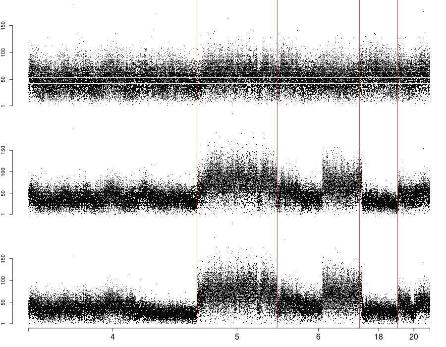
Refer to caption
Fig S3.3: Raw whole genome sequencing data from cell line LS411
Refer to caption
Fig S3.4: Preprocessed whole genome sequencing data from cell line LS411
Refer to caption
Fig S3.5: SLAM’s estimates (red lines) for qn​(α)=−0.15q_{n}(\alpha)=-0.15 (selected with MVT-method from Section 4.6) and qn​(β)=2.2q_{n}(\beta)=2.2. Top row: total copy-number estimates across the genome. Rows 2-4: estimates of the CN profiles of the germline and clones.

S4 Data driven selection of qn​(α)q_{n}(\alpha)

In the following we give further details on the SST-method for selection of qn​(α)q_{n}(\alpha) introduced in Section 4.6. To simplify notation let nn be even. Then Y1:⁣=(Y1,Y3,…,Yn−1)Y^{1}\mathrel{\mathop{:}\!\!=}(Y_{1},Y_{3},\ldots,Y_{n-1}) and Y2:⁣=(Y2,Y4,…,Yn)Y^{2}\mathrel{\mathop{:}\!\!=}(Y_{2},Y_{4},\ldots,Y_{n}) are both samples of size n/2n/2 from the same underlying mixture gg, with corresponding estimates ω^q1:⁣=ω^(Y1,q)\hat{\omega}^{1}_{q}\mathrel{\mathop{:}\!\!=}\hat{\omega}(Y^{1},q) and ω^q2:⁣=ω^(Y2,q)\hat{\omega}^{2}_{q}\mathrel{\mathop{:}\!\!=}\hat{\omega}(Y^{2},q), respectively. Let LL be a loss function and h(q):⁣=E[L(ω^q−ω)]h(q)\mathrel{\mathop{:}\!\!=}\operatorname{E}[L(\hat{\omega}_{q}-\omega)] its corresponding performance measure for estimating ω\omega, e.g., the MSE with L=∥⋅∥22L=\|\cdot\|^{2}_{2}, which is to be minimized. As ω\omega is unknown, h⁡(q)h(q) has to be estimated. This is done by

h^(q):⁣=12(L(ω^q−ω^q1)+L(ω^q−ω^q2))\displaystyle\hat{h}(q)\mathrel{\mathop{:}\!\!=}\frac{1}{2}\left(L(\hat{\omega}_{q}-\hat{\omega}^{1}_{q})+L(\hat{\omega}_{q}-\hat{\omega}^{2}_{q})\right)

and we estimate the minimizing qq of hh as

q^:⁣=argminq≤q0h^(q).\displaystyle\hat{q}\mathrel{\mathop{:}\!\!=}\operatorname{argmin}_{q\leq q_{0}}\hat{h}(q). (77)

Bounding qq from above by q0q_{0} is necessary as for q→∞q\rightarrow\infty, i.e. α→0\alpha\rightarrow 0, the corresponding confidence region 𝒞1−α\mathcal{C}_{1-\alpha} converges to the entire domain Ω⁡(m)\Omega(m), hence h⁡(q)→0h(q)\rightarrow 0 as q→∞q\rightarrow\infty. We found empirically that q0:⁣=qn(0.01)q_{0}\mathrel{\mathop{:}\!\!=}q_{n}(0.01) serves as a good bound (as statements with higher confidence as 0.990.99 are rarely demanded), also to reduce computation time for the optimization of (77).

Refer to caption
Fig S4.1: Pointwise mean of 1,0001,000 replications of ‖ω^q−ω‖2\|\hat{\omega}_{q}-\omega\|_{2}, ‖ω^q−ω‖1\|\hat{\omega}_{q}-\omega\|_{1}, respectively (black) and of (‖ω^q1−ω^q‖2+‖ω^q2−ω^q‖2)\left(\|\hat{\omega}^{1}_{q}-\hat{\omega}_{q}\|_{2}+\|\hat{\omega}^{2}_{q}-\hat{\omega}_{q}\|_{2}\right), (‖ω^q1−ω^q‖1+‖ω^q2−ω^q‖1)\left(\|\hat{\omega}^{1}_{q}-\hat{\omega}_{q}\|_{1}+\|\hat{\omega}^{2}_{q}-\hat{\omega}_{q}\|_{1}\right), respectively (red) (from left to right), for the setting as in Example 1.1 with n=1280n=1280 and σ=0.05\sigma=0.05. The vertical lines indicate the corresponding minima.
Refer to caption
Fig S4.2: MISE and MIAE of f^q1\hat{f}^{1}_{q} (black), f^q2\hat{f}^{2}_{q} (blue), and f^q3\hat{f}^{3}_{q} (red) observed from 1,0001,000 realizations for the setting as in Example 1.1 with n=1280n=1280 and σ=0.05\sigma=0.05. The vertical dotted line indicates qn​(0.01)=2.07q_{n}(0.01)=2.07.

The performance of the selector in (77) is illustrated for the setting of Example 1.1 (with n=1280n=1280 and σ=0.05\sigma=0.05) in Figure S4.1 for the MSE(qq) (L=∥⋅∥22L=\|\cdot\|_{2}^{2}) and the MAE(qq) (L=∥⋅∥1L=\|\cdot\|_{1}), respectively. From this we find that the optimal qq (the minimizer of the black line) is quite well approximated by its estimate q^≈0.5\hat{q}\approx 0.5 (the minimizer of the red line). Simulations for different nn and σ\sigma with σ/n\sigma/\sqrt{n} in the order of our application example (see Section 4) show the same. Recall from the previous Section 4.3 that ω\omega is estimated quite stable for a range of qq. In Figure S4.1 q≈0.5q\approx 0.5 corresponds to α≈0.69\alpha\approx 0.69. The optimal qq for the MSE is q≈0.35q\approx 0.35, corresponding to α≈0.81\alpha\approx 0.81 and for the MAE q≈0.1q\approx 0.1, corresponding to α≈0.95\alpha\approx 0.95.

For large noise levels, however, we found that the SST-selection method is outperformed by the MVT-method from Section 4.6 illustrated for the setting of Example 1.1 with n=1280n=1280 and σ=0.05,0.08,0.1,0.2\sigma=0.05,0.08,0.1,0.2 in Table S4.1.

Table S4.1: MSE and MAE for the SST-method and the MVT-method for the setting of Example 1.1 with n=1280n=1280 and σ=0.05,0.08,0.1,0.2\sigma=0.05,0.08,0.1,0.2 obtained from 2,0002,000 replications.
MSE [10−4][10^{-4}] MAE [10−3][10^{-3}]
SST MVT SST MVT
σ=0.05\sigma=0.05 44 44 2727 1818
σ=0.08\sigma=0.08 2626 3434 7373 8181
σ=0.1\sigma=0.1 5656 3030 110110 7878
σ=0.2\sigma=0.2 166166 4444 206206 9595