跳到论文正文
W Papers独立论文阅读器 arXiv:1608.07145 论文正文 计算阅读时间 · 0%
引用这篇论文根据当前论文元数据生成,正式投稿前建议核对。


License: arXiv.org perpetual non-exclusive license
arXiv:1608.07145v2 [hep-ph] 30 Aug 2016

Semi-leptonic Production of Ds​J​(3040)D_{sJ}(3040) and DJ​(3000)D_{J}(3000) in BsB_{s} and BB Decays

Si-chen Li[1], Yue Jiang[1], Tian-hong Wang[1], Qiang Li[1], Zhi-hui Wang[2], Guo-Li Wang[1] Note: jiangure@hit.edu.cn Address: 1Department of Physics, Harbin Institute of Technology, Harbin, 150001
2School of Electrical & Information Engineering, Beifang University of Nationalities, Yinchuan, 750021
Abstract

In this paper, we study the productions of the newly detected states Ds​J​(3040)D_{sJ}(3040) and DJ​(3000)D_{J}(3000) observed by BABAR Collaboration and LHCb Collaboration. We assume these states to be the Ds​(2​P)D_{s}(2P) and D⁡(2​P)D(2P) states with the quantum number JP=1+J^{P}=1^{+} in our work. The results of improved Bethe-Salpeter method indicate that the semi-leptonic decays via BsB_{s} and BB into Ds​J​(3040)D_{sJ}(3040) and DJ​(3000)D_{J}(3000) have considerable branching ratios, for example, Br(B¯s0→D(3040)+s​Je−ν¯e\overline{B}_{s}^{0}\rightarrow D{{}_{sJ}^{+}}(3040)e^{-}\overline{\nu}{{}_{e}})=5.79×10−45.79\times 10^{-4}, Br(B¯0→DJ+(3000)e−ν¯e\overline{B}^{0}\rightarrow D_{J}^{+}(3000)e^{-}\overline{\nu}{{}_{e}})=2.63×10−42.63\times 10^{-4}, which shows that these semi-leptonic decays can be accessible in experiments.

Keywords: Ds​J​(3040)D_{sJ}(3040); DJ​(3000)D_{J}(3000); Semi-leptonic Decay; Improved Bethe-Salpeter Method.

I INTRODUCTION

The studys of charmed and charmed-strange mesons have made great progress in recent years, which intrigues great deal of interests in revealing their properties. More and more new resonances have been observed in experiments. For example, in charmed-strange family, Ds​1∗​(2700)±D_{s1}^{*}(2700)^{\pm} was reported by Belle Collaboration through the cascaded decay B+→D¯0​Ds​1→D¯0​D0​K+B^{+}\rightarrow\overline{D}^{0}D_{s1}\rightarrow\overline{D}^{0}D^{0}K^{+} and identified as a 1−1^{-} assignment [1], and Ds​J∗​(2860)±D_{sJ}^{*}(2860)^{\pm} was discovered by BABAR Collaboration in Ds​J​(2860)→D0​K+,D+​Ks0D_{sJ}(2860)\rightarrow D^{0}K^{+},D^{+}K_{s}^{0} [2], which is very likely to be 3−3^{-} state. In charmed family, D⁡(2550)D(2550), D⁡(2600)D(2600), D⁡(2750)D(2750), D⁡(2760)D(2760) were observed by BaBar Collaboration with analysis of helicity distribution [3]. (D⁡(2550)D(2550), D⁡(2600)D(2600)) are tentatively identified as 2S doublet (0−,1−)(0^{-},1^{-}) while D⁡(2750)D(2750) and D⁡(2760)D(2760) are 1​D1D doublet (2−2^{-}, 3−3^{-}) [4]. Recently, two new resonances have been detected experimentally with masses around 30003000 MeV, Ds​JD_{sJ}(3040)+ was observed in the D∗​KD^{*}K invariant mass spectrum in inclusive e+​e−e^{+}e^{-} collision by BABAR [5], which is a good candidate as the radial excitation of Ds​1​(2460)+D_{s1}(2460)^{+} [6]. In D+​π−D^{+}\pi^{-} and D0​π+D^{0}\pi^{+} mass spectra, DJ​(3000)0D_{J}(3000)^{0} was observed by LHCb Collaboration [7], which could be interpreted as the radial excitation of D1​(2430)0D_{1}(2430)^{0}, and their masses and full widths are [5, 7]

mDs​J​(3040)+=(3044±8−5+30)​MeV,ΓDs​J​(3040)+=(239±35−42+46)​MeV,mDJ​(3000)0=(2971.8±8.7)​MeV,ΓDJ​(3000)0=(188.1±44.8)​MeV.\displaystyle\begin{aligned} m_{D_{sJ}(3040)^{+}}=\left(3044\pm 8^{+30}_{-5}\right)\mathrm{MeV},\\ \varGamma_{D_{sJ}(3040)^{+}}=\left(239\pm 35^{+46}_{-42}\right)\mathrm{MeV},\\ m_{D_{J}(3000)^{0}}=\left(2971.8\pm 8.7\right)\mathrm{MeV},\\ \varGamma_{D_{J}(3000)^{0}}=\left(188.1\pm 44.8\right)\mathrm{MeV}.\\ \end{aligned} (1)

Regarding to the topic of radial excited states of DsD_{s} and DD mesons, several works have been done about their mass spectra and strong decays [8, 9, 10, 11]. One thing drawing our attention is that no other heavy-light 2​P2P state has been confirmed by experiment except charmonium and bottomonium, which means the study of charmed and charmed-strange 2​P2P states will enlarge our knowledge of bound states and deepen the understanding of nonperturbative QCD.

We notice that Ds​J​(3040)D_{sJ}(3040) and DJ​(3000)D_{J}(3000), assumed to be radial excitation of Ds​1​(2460)D_{s1}(2460) and D1​(2430)D_{1}(2430) in recent studies, can be produced via the semileptonic decays of BsB_{s} and BB, which are different from the observed production processes. Previous studies show that semi-leptonic decays could be a good platform to produce charmed and charmed-strange mesons, for instance, the process of Bs→Ds​1​(2460)​l​ν¯lB_{s}\rightarrow D_{s1}(2460)l\overline{\nu}_{l} has been calculated through relativistic quark model based on the quasipotential approach [12], three point QCD sum rule methods [13], QCD sum rules under HQET [14], constituent quark meson model [15], and instantaneous Bethe-Salpeter method [16]. The same order 10−310^{-3} of the results in various models indicates that semi-leptonic decays have considerable branching ratios. In addition, the study of semi-leptonic decay provide an extra source of information for the determination of CKM matrix elements and the relativistic quark dynamics inside heavy-light mesons. In this paper, we explore the production of Ds​J​(3040)D_{sJ}(3040) and DJ​(3000)D_{J}(3000) by the improved B-S(Bethe-Salpeter) method, and give the results of form factors as well as branching ratios.

The rest of this paper is organized in the following arrangements. In section 2 we deduce the formulation of semi-leptonic decay. The hadronic matrix elements of production are given in section 3, numerical results and discussions are presented in section 4.

II THE FORMULATIONS OF SEMI-LEPTONIC DECAY

We take B¯s0→Ds​J+​(3040)​l−​ν¯l{\overline{B}^{0}_{s}}\rightarrow D^{+}_{sJ}(3040)l^{-}\overline{\nu}_{l} as an example to illustrate this type of process. The feynman diagram of this semi-leptonic decay is drawn in figure 1.

Refer to caption
Figure 1: Feynman diagram of semi-leptonic decay B¯s0→Ds+​(2​P)​l−​νl{\overline{B}^{0}_{s}}\rightarrow D^{+}_{s}(2P)l^{-}\nu_{l}

The amplitude of B¯s0→Ds​J+​(3040)​l−​ν¯l{\overline{B}^{0}_{s}}\rightarrow D^{+}_{sJ}(3040)l^{-}\overline{\nu}_{l} is [16]

T=GF2​Vc​b​u¯​(pl)​γξ​(1−γ5)​ν​(pνl)​⟨Ds​J+​(3040)​(Pf)|Jξ|B¯s0​(P)⟩,T=\frac{G_{F}}{\sqrt{2}}V_{cb}\overline{u}(p_{l})\gamma^{\xi}(1-\gamma_{5})\nu(p_{\nu_{l}})\left\langle D_{sJ}^{+}(3040)(P_{f})|J_{\xi}|\overline{B}_{s}^{0}(P)\right\rangle, (2)

where Vc​bV_{cb} is the CKM matrix element, GFG_{F} is the fermi constant, Jξ=Vξ−AξJ_{\xi}=V_{\xi}-A_{\xi} is the charged weak current, in which Vξ=c¯​γξ​bV_{\xi}=\overline{c}\gamma_{\xi}b, Aξ=c¯​γξ​γ5​bA_{\xi}=\overline{c}\gamma_{\xi}\gamma_{5}b, PP and PfP_{f} are the momenta of the initial meson B¯s0\overline{B}_{s}^{0} and final meson Ds​J+​(3040)D_{sJ}^{+}(3040) respectively. Thus the square of the amplitude is:

|T|2=GF22​|Vb​c|2​lξ​ξ′​hξ​ξ′,|T|^{2}=\frac{G_{F}^{2}}{2}|V_{bc}|^{2}l^{\xi\xi^{\prime}}h_{\xi\xi^{\prime}}, (3)

where the leptonic tensor could be simplified as:

lξ​ξ′=8(pνlξplξ′+plξpvlξ′−pvlplgξ​ξ′+iϵξ​ξ′​α​βp1​αp2​β),l^{\xi\xi^{\prime}}=8\left(p_{\nu{{}_{l}}}^{\xi}p_{l}^{\xi^{\prime}}+p_{l}^{\xi}p_{v_{l}}^{\xi^{\prime}}-p_{v_{l}}p_{l}g^{\xi\xi^{\prime}}+i\epsilon^{\xi\xi^{\prime}\alpha\beta}p_{1\alpha}p_{2\beta}\right), (4)

and hadronic tensor is defined as:

hξ​ξ′=⟨B¯s0​(P)|Jξ†|Ds​J+​(3040)​(Pf)⟩​⟨Ds​J+​(3040)​(Pf)|Jξ′|B¯s0​(P)⟩,h_{\xi\xi^{\prime}}=\left\langle\overline{B}_{s}^{0}(P)|J_{\xi}^{\dagger}|D_{sJ}^{+}(3040)(P_{f})\right\rangle\left\langle D_{sJ}^{+}(3040)(P_{f})|J_{\xi^{\prime}}|\overline{B}_{s}^{0}(P)\right\rangle, (5)

which can be described as form factors. Explicit forms are present in next subsection.

III HADRONIC MATRIX ELEMENT OF SEMI-LEPTONIC DECAY

The calculation of hadronic matrix element is model-dependent. In this paper, we determine the hadronic matrix element through the instantaneous Bethe-Salpeter method with Mandelstam formalism. As a relativistic quark model, the instantaneous Bethe-Salpeter method has been applied in many transitions among heavy-light mesons. More details about instantaneous Bethe-Salpeter equation are given in Appendix A.

Regarding to the classification of heavy-light meson, the heavy-light mesons can be classified in doublets based on the total angular momentum of the light quark sls_{l}. We can categorize the heavy mesons into several doublets, for example, the S doublet is (0+,1+)(0^{+},1^{+}) with sl=12s_{l}=\frac{1}{2} , and the T doublet is (1+,2+)(1^{+},2^{+}) with sl=32s_{l}=\frac{3}{2} , thus the 1+1^{+} states can be labeled as P11/2P_{1}^{1/2} and P13/2P_{1}^{3/2}. But in our method, we solved the Salpeter equation and obtained the wave functions of the P13{}^{3}P_{1} and P11{}^{1}P_{1} states, whose forms are given in Appendix B, then the physical states are mixtures of the P13{}^{3}P_{1} and P11{}^{1}P_{1}:

|32⟩=cosθ|1P1⟩+sinθ|3P1⟩,\displaystyle\left|\frac{3}{2}\right\rangle={\cos{\theta}}\left|{}^{1}P_{1}\right\rangle+{\sin{\theta}}\left|{}^{3}P_{1}\right\rangle, (6)
|12⟩=−sinθ|1P1⟩+cosθ|3P1⟩.\displaystyle\left|\frac{1}{2}\right\rangle=-{\sin{\theta}}\left|{}^{1}P_{1}\right\rangle+{\cos{\theta}}\left|{}^{3}P_{1}\right\rangle.

In the heavy quark limit, which is mQ→∞m_{Q}\rightarrow\infty, the mixing angle θ≈35.3∘\theta\approx 35.3^{\circ} [17]. Ds​J​(3040)D_{sJ}(3040) is assumed to be the radial excitation of Ds​1​(2460)D_{s1}(2460) in this paper, which is P11/2P_{1}^{1/2} state. The partner has not been discovered yet, which is correspondent to P13/2P_{1}^{3/2} state. By the B-S method with the instantaneous approach, the hadronic matrix element can be written as the overlapping integral over the initial and final B-S wave functions [16]:

⟨Ds​J+​(Pf)​(P11)|Jξ|B¯s0​(P)⟩\displaystyle\left\langle D_{sJ}^{+}\left(P_{f}\right)\left({}^{1}{P}_{1}\right)|J_{\xi}|\overline{B}_{s}^{0}\left(P\right)\right\rangle =i​∫d4​q(2​π)4​Tr​[χ¯Ds​J​(Pf,P,q1)​(α1​P̸+q̸−ms)​γξ​(1−γ5)​χBs0​(P,q)]\displaystyle=i\int\frac{{\rm d}^{4}q}{(2\pi)^{4}}{\rm{Tr}}\left[\overline{\chi}_{D_{sJ}}(P_{f},P,q_{1})(\alpha_{1}\not{P}+\not{q}-m_{s})\gamma_{\xi}(1-\gamma_{5})\chi_{B_{s}^{0}}(P,q)\right] (7)
=∫d​q→(2​π)3​Tr​[φ¯1++⁣+​(P11)​(q→1)​γξ​(1−γ5)​φ0−+⁣+​(q→)​P̸M]\displaystyle=\int\frac{{\rm d}\vec{q}}{(2\pi)^{3}}{\rm{Tr}}\left[\overline{\varphi}_{1^{+}}^{++}\left({}^{1}{P}_{1}\right)\left(\vec{q}_{1}\right)\gamma_{\xi}\left(1-\gamma_{5}\right){\varphi}_{0^{-}}^{++}\left(\vec{q}\right)\frac{\not{P}}{M}\right]
=ϵμ​(t1​Pξ​Pμ+t2​Pf​ξ​Pμ+t3​gξμ+t4​ϵξP​P1​μ),\displaystyle=\epsilon_{\mu}\left(t_{1}P_{\xi}P^{\mu}+t_{2}P_{f\xi}P^{\mu}+t_{3}g^{\;\;\mu}_{\xi}+t_{4}\epsilon^{\;\;PP_{1}\mu}_{\xi}\right),
⟨Ds​J+​(Pf)​(P13)|Jξ|B¯s0​(P)⟩\displaystyle\hskip-50.58878pt\left\langle D_{sJ}^{+}(P_{f})\left({}^{3}{P}_{1}\right)|J_{\xi}|\overline{B}_{s}^{0}(P)\right\rangle =∫d​q→(2​π)3​Tr​[φ¯1++⁣+​(P13)​(q→1)​γξ​(1−γ5)​φ0−+⁣+​(q→)​P̸M]\displaystyle=\int\frac{{\rm d}\vec{q}}{(2\pi)^{3}}{\rm{Tr}}\left[\overline{\varphi}_{1^{+}}^{++}\left({}^{3}{P}_{1}\right)\left(\vec{q}_{1}\right)\gamma_{\xi}\left(1-\gamma_{5}\right){\varphi}_{0^{-}}^{++}(\vec{q})\frac{\not{P}}{M}\right] (8)
=ϵμ​(t5​Pξ​Pμ+t6​Pf​ξ​Pμ+t7​gξμ+t8​ϵξP​P1​μ),\displaystyle=\epsilon_{\mu}\left(t_{5}P_{\xi}P^{\mu}+t_{6}P_{f\xi}P^{\mu}+t_{7}g^{\;\;\mu}_{\xi}+t_{8}\epsilon^{\;\;PP_{1}\mu}_{\xi}\right),

where q→\vec{q} and q→1\vec{q}_{1} are relative three-momentum between the quark and anti-quark for initial state and final state. t1t_{1} to t8t_{8} are the form factors, which are given in Appendix C.

The wave functions we adopt above are for P11{}^{1}P_{1} and P13{}^{3}P_{1} states. Due to the mixture of physical states, the form factors for P1/2P^{1/2} and P3/2P^{3/2} states are given as:

xi+4=ti​cos⁡θ+ti+4​sin⁡θ,xi=−ti​sin⁡θ+ti+4​cos⁡θ,\displaystyle\begin{aligned} x_{i+4}=t_{i}\cos\theta+t_{i+4}\sin\theta,\\ x_{i}=-t_{i}\sin\theta+t_{i+4}\cos\theta,\end{aligned} (9)

where i=1,2,3,4.i=1,2,3,4.

Another thing we should notice is that the masses of P11{}^{1}P_{1} and P13{}^{3}P_{1} are different from P1/2P^{1/2} and P3/2P^{3/2}. There is also a mixture between them and the relation is given as [18]:

mP112=m122​sin2⁡θ+m322​cos2⁡θ,mP132=m122​cos2⁡θ+m322​sin2⁡θ.\displaystyle\begin{aligned} &m^{2}_{{}^{1}P_{1}}=m^{2}_{\frac{1}{2}}\sin^{2}\theta+m^{2}_{\frac{3}{2}}\cos^{2}\theta,\\ &m^{2}_{{}^{3}P_{1}}=m^{2}_{\frac{1}{2}}\cos^{2}\theta+m^{2}_{\frac{3}{2}}\sin^{2}\theta.\end{aligned} (10)

By giving the form factors, the width of semi-leptonic decay is

Γ=GF2​Vc​b2​M332​π3∫plEldp→l∫pfEfdp→f{2α(yM2)+β+⁣+[4(2x(1−Mf2M2+y)−4x2−y)+ml2M2(8x+4Mf2M2−3y−ml2M2)]+(β±+β∓)ml2M2(2−4x+y−2Mf2M2)+β−⁣−ml2M2(y−ml2M2)+2γ[y(1−4x+y−Mf2M2)+Ml2M2(1+y−Mf2M2)]},\displaystyle\begin{aligned} \varGamma=&\frac{G_{F}^{2}V_{cb}^{2}M^{3}}{32\pi^{3}}\int\frac{p_{l}}{E_{l}}{\rm d}\vec{p}_{l}\int\frac{p_{f}}{E_{f}}{\rm d}\vec{p}_{f}\left\{2\alpha\left(\frac{y}{M^{2}}\right)+\beta_{++}\left[4\left(2x\left(1-\frac{M_{f}^{2}}{M^{2}}+y\right)-4x^{2}-y\right)\right.\right.\\ &\left.\left.+\frac{m_{l}^{2}}{M^{2}}\left(8x+4\frac{M_{f}^{2}}{M^{2}}-3y-\frac{m_{l}^{2}}{M^{2}}\right)\right]+\left(\beta_{\pm}+\beta_{\mp}\right)\frac{m_{l}^{2}}{M^{2}}\left(2-4x+y-2\frac{M_{f}^{2}}{M^{2}}\right)\right.\\ &\left.+\beta_{--}\frac{m_{l}^{2}}{M^{2}}\left(y-\frac{m_{l}^{2}}{M^{2}}\right)+2\gamma\left[y\left(1-4x+y-\frac{M_{f}^{2}}{M^{2}}\right)+\frac{M_{l}^{2}}{M^{2}}\left(1+y-\frac{M_{f}^{2}}{M^{2}}\right)\right]\right\},\end{aligned} (11)

where MfM_{f} and MM are masses of the final and initial meson respectively, mlm_{l} is the mass of the corresponding lepton. α\alpha, β±⁣±\beta_{\pm\pm} and γ\gamma are coefficients as functions of the form factors:

x=ElM,y=(p−pf)2M2,\displaystyle x=\frac{E_{l}}{M},y=\frac{\left(p-p_{f}\right)^{2}}{M^{2}}, (12)
α=x32+x42​M2​pf2,\displaystyle\alpha=x_{3}^{2}+x_{4}^{2}M^{2}p_{f}^{2},
β+⁣+=pf2​(x1+x2)24​Mf2+(2​M​Ef−M2−Mf2)​x424+x324​Mf2+(M​EMf2−1)​(x1+x2)​x32​M,\displaystyle\beta_{++}=p_{f}^{2}\frac{\left(x_{1}+x_{2}\right)^{2}}{4M_{f}^{2}}+\frac{\left(2ME_{f}-M^{2}-M_{f}^{2}\right)x_{4}^{2}}{4}+\frac{x_{3}^{2}}{4M_{f}^{2}}+\left(\frac{ME}{M_{f}^{2}}-1\right)\frac{\left(x_{1}+x_{2}\right)x_{3}}{2M},
β+⁣−=β−⁣+=pf2​(x1+x2)​(x1−x2)4​Mf2+(M2−Mf2)4−(x1+x2​E​MMf2)​x32​M−x324​Mf2,\displaystyle\beta_{+-}=\beta_{-+}=p_{f}^{2}\frac{(x_{1}+x_{2})(x_{1}-x_{2})}{4M_{f}^{2}}+\frac{\left(M^{2}-M_{f}^{2}\right)}{4}-\left(x_{1}+\frac{x_{2}EM}{M_{f}^{2}}\right)\frac{x_{3}}{2M}-\frac{x_{3}^{2}}{4M_{f}^{2}},
β−⁣−=pf2​(x1−x2)24​Mf2−(2​M​E+Mf2+M2)​x424+x324​Mf2+(1+M​EMf2)​(x2−x1)​x32​M,\displaystyle\beta_{--}=p_{f}^{2}\frac{\left(x_{1}-x_{2}\right)^{2}}{4M_{f}^{2}}-\frac{\left(2ME+M_{f}^{2}+M^{2}\right)x_{4}^{2}}{4}+\frac{x_{3}^{2}}{4M_{f}^{2}}+\left(1+\frac{ME}{M_{f}^{2}}\right)\frac{\left(x_{2}-x_{1}\right)x_{3}}{2M},
γ=−x3​x4.\displaystyle\gamma=-x_{3}x_{4}.

IV NUMERICAL RESULTS AND ANALYSIS

IV.1 form factors

In our model, the input parameters of calculation are chosen as following: λ\lambda =0.21 GeV2, ΛQCD\varLambda_{\rm QCD}=0.27 GeV, a=e=2.71, α\alpha=0.06 GeV, mbm_{b}=4.96 GeV, msm_{s}=0.50 GeV, mcm_{c}=1.62 GeV, mdm_{d}=0.311 GeV, which are the best results to fit the mass spectrum of related mesons [19]. For semi-leptonic decay, we also need CKM matrix elements: Vb​cV_{bc}=0.0406, and the lifetime of initial meson τBs​0=1.469×10⁻¹²\tau_{B_{s0}}=1.469\times 10^{-12} s, the masses of mB0m_{B^{0}}=5279.58 MeV and mBs0m_{B^{0}_{s}}=5366.77 MeV are taken from PDG [20]. We notice that the partners of Ds​J​(3040)D_{sJ}(3040) and DJ​(3000)D_{J}(3000) are not discovered yet, the masses required in our calculation are taken as 3022.3 MeV and 2913.8 MeV for Ds​(2​P13/2)D_{s}(2P^{3/2}_{1}) and D⁡(2​P13/2)D(2P^{3/2}_{1}) respectively. Varying all the input parameters simultaneously within ±\pm 5% of the central values, we obtain the uncertainties of branching ratios.

Refer to caption
Refer to caption
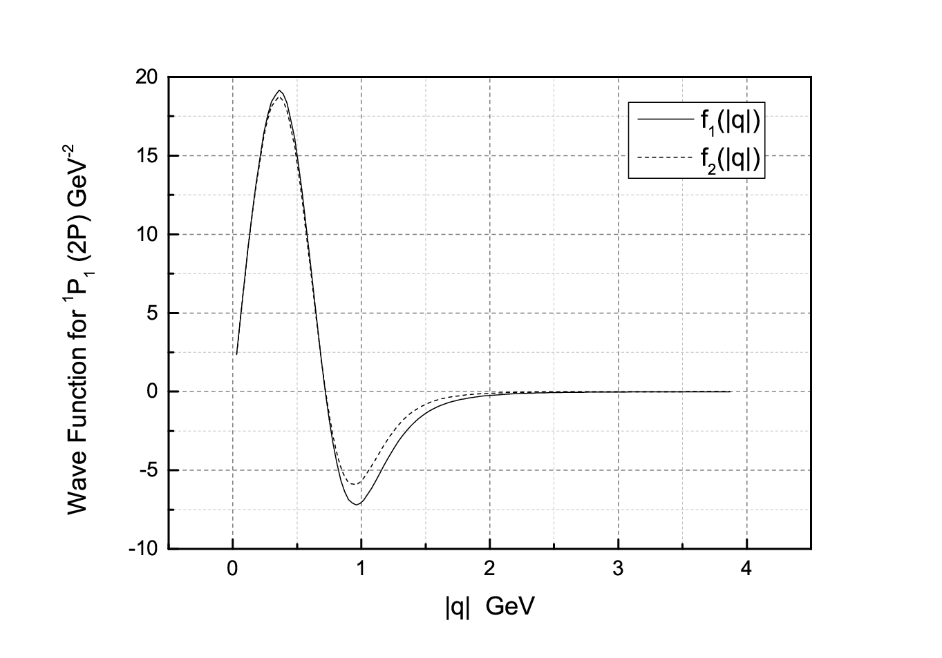
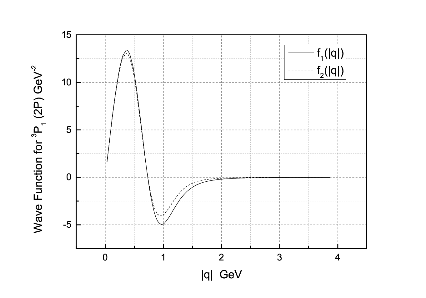
Figure 2: The wavefunctions of P11{}^{1}P_{1} and P13{}^{3}P_{1} for Ds​(2​P)D_{s}(2P) meson

To show the numerical results of wave functions explicitly, we plot the P11{}^{1}P_{1} and P13{}^{3}P_{1} state for Ds​(2​P)D_{s}(2P) meson in figure 2. We can see that P11{}^{1}P_{1} and P13{}^{3}P_{1} states share the same shape. As an example, The form factors x1x_{1} to x4x_{4} are shown in figure 3, where t=(P−Pf)2=M2+Mf2−2​M​Eft=(P-P_{f})^{2}=M^{2}+M_{f}^{2}-2ME_{f} and tmt_{m} is the maximum of tt.

Refer to caption
Figure 3: The form factors of B¯s0→Ds​J​(3040)+​e−​ν¯e\overline{B}^{0}_{s}\rightarrow D_{sJ}(3040)^{+}e^{-}\overline{\nu}_{e}

IV.2 branching ratios

for Ds​J​(3040)D_{sJ}(3040)

In table I, we show the branching ratios of semi-leptonic production of Ds​(2​P)+D_{s}(2P)^{+}. Generally, the cases of ee and μ\mu are 2 orders of magnitude larger than the case of τ\tau due to the phase space. We also notice that the branching ratios of B¯s0→D(P)3/21+s​Jl−ν¯l\overline{B}_{s}^{0}\rightarrow D{{}_{sJ}^{+}}(P{{}_{1}^{3/2}})l^{-}\overline{\nu}{{}_{l}} are 10 times larger than B¯s0→D(P)1/21+s​Jl−ν¯l\overline{B}_{s}^{0}\rightarrow D{{}_{sJ}^{+}}(P{{}_{1}^{1/2}})l^{-}\overline{\nu}{{}_{l}}. Ref [21] calculate the same process via covariant light-front quark model. The result in Ref [22] is obtained through modified harmonic-oscillator light-front wave function (I) and light-front quark model associated within HQET (II). We can see that our results are well consistent with the light-front quark model associated within HQET but show a little discrepancy with the other two results. All these results indicate that more theoretical researches should be done in the future.

Table 1: Branching ratios of B¯s0→Ds+​(2​P)​l−​ν¯l{\overline{B}^{0}_{s}}\rightarrow D^{+}_{s}(2P)l^{-}\overline{\nu}_{l}
ours [21] I [22] II [22]
B¯s0→D(3040)+s​Je−ν¯e\overline{B}_{s}^{0}\rightarrow D{{}_{sJ}^{+}}(3040)e^{-}\overline{\nu}{{}_{e}} (5.79−2.0+2.1)×10−4(5.79^{+2.1}_{-2.0})\times 10^{-4} (2.49−0.4+0.4)×10−4(2.49^{+0.4}_{-0.4})\times 10^{-4} 5.6×10⁻⁴{5.6\times 10^{-4}}
B¯s0→D(P)3/21+s​Je−ν¯e\overline{B}_{s}^{0}\rightarrow D{{}_{sJ}^{+}}(P{{}_{1}^{3/2}})e^{-}\overline{\nu}{{}_{e}} (2.34−1.04+1.30)×10−3(2.34^{+1.30}_{-1.04})\times 10^{-3} (2.42−0.14+0.07)×10−3(2.42^{+0.07}_{-0.14})\times 10^{-3} 1.24×10⁻³{1.24\times 10^{-3}}
B¯s0→D(3040)+s​Jμ−ν¯μ\overline{B}_{s}^{0}\rightarrow D{{}_{sJ}^{+}}(3040)\mu^{-}\overline{\nu}{{}_{\mu}} (5.77−2.07+2.15)×10−4(5.77^{+2.15}_{-2.07})\times 10^{-4} (3.5−1.0+1.1)×10−4(3.5^{+1.1}_{-1.0})\times 10^{-4} (2.46−0.42+0.4)×10−4(2.46^{+0.4}_{-0.42})\times 10^{-4} 5.6×10⁻⁴{5.6\times 10^{-4}}
B¯s0→D(P)3/21+s​Jμ−ν¯μ\overline{B}_{s}^{0}\rightarrow D{{}_{sJ}^{+}}(P{{}_{1}^{3/2}})\mu^{-}\overline{\nu}{{}_{\mu}} (2.36−1.06+1.28)×10−3(2.36^{+1.28}_{-1.06})\times 10^{-3} (4.0−0.5+0.4)×10−3(4.0^{+0.4}_{-0.5})\times 10^{-3} (2.39−0.13+0.07)×10−3(2.39^{+0.07}_{-0.13})\times 10^{-3} 1.24×10⁻³{1.24\times 10^{-3}}
B¯s0→D(3040)+s​Jτ−ν¯τ\overline{B}_{s}^{0}\rightarrow D{{}_{sJ}^{+}}(3040)\tau^{-}\overline{\nu}{{}_{\tau}} (4.07−1.74+1.95)×10−6(4.07^{+1.95}_{-1.74})\times 10^{-6} (9.9−3.5+4.4)×10−6(9.9^{+4.4}_{-3.5})\times 10^{-6} (5.2−0.5+0.4)×10−6(5.2^{+0.4}_{-0.5})\times 10^{-6}
B¯s0→D(P)3/21+s​Jτ−ν¯τ\overline{B}_{s}^{0}\rightarrow D{{}_{sJ}^{+}}(P{{}_{1}^{3/2}})\tau^{-}\overline{\nu}{{}_{\tau}} (3.49−1.78+2.39)×10−5(3.49^{+2.39}_{-1.78})\times 10^{-5} (9.7−0.8+0.8)×10−5(9.7^{+0.8}_{-0.8})\times 10^{-5} (0.43−0.01+0)×10−6(0.43^{+0}_{-0.01})\times 10^{-6}

Due to the lack of data of DsD_{s}(2PP) state, as a comparison, we give the information about 1​P1P state with JP=1+J^{P}=1^{+}. The branching ratio of cascaded decay Br(Bs0→Ds​1(2536)−μ+νμ)×(B_{s}^{0}\rightarrow D_{s1}(2536)^{-}\mu^{+}\nu_{\mu})\timesBr(Ds​1​(2536)−→D∗⁣−​Ks0CLOSE(D_{s1}(2536)^{-}\rightarrow D^{*-}K^{0}_{s} )=(2.5±0.7)×10−3(2.5\pm 0.7)\times 10^{-3}, and the branching ratio of strong decay is 0.85±0.120.85\pm 0.12 [20], so the branching ratio of semi-leptonic decay into 1​P1P state is 2.94−1.09+1.44×10−32.94^{+1.44}_{-1.09}\times 10^{-3}. The corresponding first radial excitation of Ds​1​(2536)−D_{s1}(2536)^{-} is Ds​1​(P13/2)−D_{s1}(P_{1}^{3/2})^{-}, whose production rate via semi-leptonic decay is 2.34×10−32.34\times 10^{-3} in our method [16], this may imply that our results are reliable.

Although the production ratio of Ds​J​(3040)D_{sJ}(3040) is very small in B¯s0\overline{B}^{0}_{s} semi-leptonic decay, considering that the LHCb experiment will produce more than 10610^{6} BsB_{s} mesons per running year [22], the branching ratios of B¯s0→Ds​J​(3040)+​e−​ν¯e\overline{B}^{0}_{s}\rightarrow D_{sJ}(3040)^{+}e^{-}\overline{\nu}_{e} around 10−410^{-4} are considerable, and are accessible in the current BsB_{s} decay data. So the semi-leptonic approach has a promising prospect in producing Ds​J​(3040)D_{sJ}(3040).

for DJ​(3000)D_{J}(3000)

Table 2: Branching ratios of B¯0→D+​(2​P)​l−​ν¯l\overline{B}^{0}\rightarrow D^{+}(2P)l^{-}\overline{\nu}_{l}
ours [22]
B¯0→DJ(3000)+e−ν¯e\overline{B}^{0}\rightarrow D_{J}(3000)^{+}e^{-}\overline{\nu}{{}_{e}} (2.63−0.68+0.33)×10−4(2.63^{+0.33}_{-0.68})\times 10^{-4} (2.57−0.44+0.39)×10−4({2.57^{+0.39}_{-0.44})\times 10^{-4}}
B¯0→D(2P)3/21e−+ν¯e\overline{B}^{0}\rightarrow D(2P{{}_{1}^{3/2}}){{}^{+}}e^{-}\overline{\nu}{{}_{e}} (2.62−0.50+0.64)×10−4(2.62^{+0.64}_{-0.50})\times 10^{-4} (2.72−0.11+0.02)×10−3({2.72^{+0.02}_{-0.11})\times 10^{-3}}
B¯0→DJ(3000)+μ−ν¯μ\overline{B}^{0}\rightarrow D_{J}(3000)^{+}\mu^{-}\overline{\nu}{{}_{\mu}} (2.38−0.42+0.60)×10−4(2.38^{+0.60}_{-0.42})\times 10^{-4} (2.54−0.44+0.38)×10−4(2.54^{+0.38}_{-0.44})\times 10^{-4}
B¯0→D(2P)3/21μ−+ν¯μ\overline{B}^{0}\rightarrow D(2P{{}_{1}^{3/2}}){{}^{+}}\mu^{-}\overline{\nu}{{}_{\mu}} (2.42−0.46+0.57)×10−4(2.42^{+0.57}_{-0.46})\times 10^{-4} (2.69−0.11+0.02)×10−3(2.69^{+0.02}_{-0.11})\times 10^{-3}
B¯0→DJ(3000)+τ−ν¯τ\overline{B}^{0}\rightarrow D_{J}(3000)^{+}\tau^{-}\overline{\nu}{{}_{\tau}} (1.81−0.30+0.54)×10−6(1.81^{+0.54}_{-0.30})\times 10^{-6} (5.2−0.5+0.4)×10−6(5.2^{+0.4}_{-0.5})\times 10^{-6}
B¯0→D(2P)3/21τ−+ν¯τ\overline{B}^{0}\rightarrow D(2P{{}_{1}^{3/2}}){{}^{+}}\tau^{-}\overline{\nu}{{}_{\tau}} (4.44−0.59+0.76)×10−6(4.44^{+0.76}_{-0.59})\times 10^{-6} (0.603−0.02+0)×10−4(0.603^{+0}_{-0.02})\times 10^{-4}

In table II, the results of B¯0→D+​(2​P)​l−​ν¯l\overline{B}^{0}\rightarrow D^{+}(2P)l^{-}\overline{\nu}_{l} are presented. Our results show that the branching ratios into two doublets are of the same order of 10−410^{-4} for ee and μ\mu, 10−610^{-6} for τ\tau. While the results from light front quark model [22] are the same of 10−410^{-4} for 2​P11/22P^{1/2}_{1} state, but one order of magnitude smaller than ours for 2​P13/22P^{3/2}_{1} state. To give some clues for this discrepancy, we list the results of B¯0→D+​(1​P)​l−​ν¯l\overline{B}^{0}\rightarrow D^{+}(1P)l^{-}\overline{\nu}_{l} as the comparison. In table III, we give the cascaded decay of D⁡(1​P)D(1P) states, in which the D1​(2430)D_{1}(2430) and D1​(2420)D_{1}(2420) are D⁡(1​P11/2)D(1P_{1}^{1/2}) and D⁡(1​P13/2)D(1P_{1}^{3/2}) respectively.

Considering that the strong decays of D1D_{1} state are dominant channels at around 67%67\% due to the isospin symmetry, one thing we should notice in table III is that for D1​(1​P13/2CLOSED_{1}(1P^{3/2}_{1}) and D1​(1​P11/2CLOSED_{1}(1P^{1/2}_{1}), the branching ratios of semi-leptonic productions are almost the same of 4.5×10−34.5\times 10^{-3} in experiment. Our results are consistent with this data. If the behaviors of 2​P2P states are similar to 1​P1P states, our results seem to be more reasonable.

Table 3: Cascaded decay of B¯0\overline{B}^{0} into D−​(1​P)D^{-}(1P)
ours exp[20]
Br(B¯0→D1(2430)−l+ν¯)l×Br(D1(2430)−→D¯∗0π−){\rm Br}(\overline{B}^{0}\rightarrow D_{1}(2430)^{-}l^{+}\overline{\nu}{{}_{l}})\times{\rm Br}(D_{1}(2430)^{-}\rightarrow\overline{D}^{*0}\pi^{-}) 3.92−0.39+0.30×10−33.92^{+0.30}_{-0.39}\times 10^{-3} (3.1±0.9)×10−3{(3.1\pm 0.9)\times 10^{-3}}
Br(B¯0→D1(2420)−l+ν¯)l×Br(D1(2420)−→D¯∗0π−){\rm Br}(\overline{B}^{0}\rightarrow D_{1}(2420)^{-}l^{+}\overline{\nu}{{}_{l}})\times{\rm Br}(D_{1}(2420)^{-}\rightarrow\overline{D}^{*0}\pi^{-}) 5.51−0.14+0.07×10−35.51^{+0.07}_{-0.14}\times 10^{-3} (2.80±0.28)×10−3{(2.80\pm 0.28)\times 10^{-3}}

Similar with Bs0→Ds+​(2​P)​l−​ν¯lB^{0}_{s}\rightarrow D^{+}_{s}(2P)l^{-}\overline{\nu}_{l}, the branching ratios are large enough to be observed in experiment, so we suggest that the LHCb and Belle II Collaboration carry out the study of semi-leptonic decays above.

The possible sources of the uncertainty on the results may come from these following factors: (1) The spin partners of DJ​(3000)D_{J}(3000) and Ds​J​(3040)D_{sJ}(3040) are not detected experimentally yet. In our work, the masses of D⁡(2​P13/2)D(2P^{3/2}_{1}) and Ds​(2​P13/2)D_{s}(2P^{3/2}_{1}) are assumed to be around 3000 MeV and 2913 MeV. It is one of the important sources of uncertainty. (2) P1/2P^{1/2} and P3/2P^{3/2} states are mixture of P11{}^{1}P_{1} and P13{}^{3}P_{1} states. The mixing equation we use in this paper is determined by the mixing angle, and this angle we use is derived from heavy-quark limit, which deviates from the realistic mixing angle, especially for the higher radial excitations [23]. That is another possible way for the uncertainty to be increased. These sources show that there are a lot of researches to be done in the future to reduce the uncertainty and make the prediction more precise.

for 3​P3P states

Although no 3​P3P state of DsD_{s} or DD meson has been observed in experiment yet, we give a very preliminary prediction in our method. The masses we used are 3421 MeV and 3427 MeV for Ds​(31​P1)D_{s}(3^{1}P_{1}) and Ds​(33​P1)D_{s}(3^{3}P_{1}) states, 3215 MeV and 3220 MeV for D⁡(31​P1)D(3^{1}P_{1}) and D⁡(33​P1)D(3^{3}P_{1}) states, which are predicted in our model. The mixing angles θ≈35.3∘\theta\approx 35.3^{\circ}. The results are given in table IV.

Table 4: Branching ratios of 3​P3P states of DsD_{s} and DD meson
Br Br
B¯s0→Ds(3P)1/21+e−ν¯e\overline{B}_{s}^{0}\rightarrow D_{s}(3P{{}_{1}^{1/2}})^{+}e^{-}\overline{\nu}{{}_{e}} (7.24−2.18+2.65)×10−6(7.24^{+2.65}_{-2.18})\times 10^{-6} B¯0→D(3P)1/21+e−ν¯e\overline{B}^{0}\rightarrow D(3P{{}_{1}^{1/2}})^{+}e^{-}\overline{\nu}{{}_{e}} (2.35−0.28+0.29)×10−6(2.35^{+0.29}_{-0.28})\times 10^{-6}
B¯s0→Ds(3P)3/21e−+ν¯e\overline{B}_{s}^{0}\rightarrow D_{s}(3P{{}_{1}^{3/2}}){{}^{+}}e^{-}\overline{\nu}{{}_{e}} (2.70−0.31+0.40)×10−4(2.70^{+0.40}_{-0.31})\times 10^{-4} B¯0→D(3P)3/21e−+ν¯e\overline{B}^{0}\rightarrow D(3P{{}_{1}^{3/2}}){{}^{+}}e^{-}\overline{\nu}{{}_{e}} (3.48−0.12+0.15)×10−4(3.48^{+0.15}_{-0.12})\times 10^{-4}
B¯s0→Ds(3P)1/21+μ−ν¯μ\overline{B}_{s}^{0}\rightarrow D_{s}(3P{{}_{1}^{1/2}})^{+}\mu^{-}\overline{\nu}{{}_{\mu}} (7.32−2.21+2.69)×10−6(7.32^{+2.69}_{-2.21})\times 10^{-6} B¯0→D(3P)1/21+μ−ν¯μ\overline{B}^{0}\rightarrow D(3P{{}_{1}^{1/2}})^{+}\mu^{-}\overline{\nu}{{}_{\mu}} (2.36−0.28+0.29)×10−6(2.36^{+0.29}_{-0.28})\times 10^{-6}
B¯s0→Ds(3P)3/21μ−+ν¯μ\overline{B}_{s}^{0}\rightarrow D_{s}(3P{{}_{1}^{3/2}}){{}^{+}}\mu^{-}\overline{\nu}{{}_{\mu}} (2.68−0.31+0.40)×10−4(2.68^{+0.40}_{-0.31})\times 10^{-4} B¯0→D(3P)3/21μ−+ν¯μ\overline{B}^{0}\rightarrow D(3P{{}_{1}^{3/2}}){{}^{+}}\mu^{-}\overline{\nu}{{}_{\mu}} (3.47−0.12+0.14)×10−4(3.47^{+0.14}_{-0.12})\times 10^{-4}
B¯s0→Ds(3P)1/21+τ−ν¯τ\overline{B}_{s}^{0}\rightarrow D_{s}(3P{{}_{1}^{1/2}})^{+}\tau^{-}\overline{\nu}{{}_{\tau}} (7.36−2.09+2.33)×10−10(7.36^{+2.33}_{-2.09})\times 10^{-10} B¯0→D(3P)1/21+τ−ν¯τ\overline{B}^{0}\rightarrow D(3P{{}_{1}^{1/2}})^{+}\tau^{-}\overline{\nu}{{}_{\tau}} (7.35−0.87+0.85)×10−9(7.35^{+0.85}_{-0.87})\times 10^{-9}
B¯s0→Ds(3P)3/21τ−+ν¯τ\overline{B}_{s}^{0}\rightarrow D_{s}(3P{{}_{1}^{3/2}}){{}^{+}}\tau^{-}\overline{\nu}{{}_{\tau}} (1.62−0.14+0.18)×10−7(1.62^{+0.18}_{-0.14})\times 10^{-7} B¯0→D(3P)3/21τ−+ν¯τ\overline{B}^{0}\rightarrow D(3P{{}_{1}^{3/2}}){{}^{+}}\tau^{-}\overline{\nu}{{}_{\tau}} (1.17−0.05+0.06)×10−6(1.17^{+0.06}_{-0.05})\times 10^{-6}

In table IV, the branching ratios of 3​P3P states are much lower than those of 2​P2P states, which presents challenges in current experiment. In addition, we see an interesting result that two mixing 3​P3P states of DD meson show discrepancy in semi-leptonic decay of B¯0\overline{B}^{0}, which needs more data and researches to give a more precise result.

V SUMMARY

The accumulative data of charmed and charmed-strange mesons are becoming more and more abundant with the running of colliders. The study of higher radial excitation in charmed and charmed-strange families is becoming a intriguing field. Two of the newly detected states are Ds​J​(3040)+D_{sJ}(3040)^{+} and DJ​(3000)0D_{J}(3000)^{0}, which are very likely to be Ds​(2​P)D_{s}(2P) and D⁡(2​P)D(2P) states. The productions of these states in experiment are the inclusive e+​e−e^{+}e^{-} interaction and D​πD\pi channel.

Under the instantaneous Bethe-Salpeter framework, we have studied the branching ratios of semi-leptonic decays into Ds​J​(3040)D_{sJ}(3040) and DJ​(3000)D_{J}(3000). Our results indicate that the semileptonic production from BsB_{s} and BB can be a good platform to produce considerable amount of Ds​J​(3040)D_{sJ}(3040) and DJ​(3000)D_{J}(3000), so we urge that relevant experiment groups could focus on these channels. Those phenomenological investigations are important to further experimentally study of 2​P2P state of DsD_{s} and DD meson.

Acknowledgements

This work was supported in part by the National Natural Science Foundation of China (NSFC) under Grant Nos. 11505039, 11575048, 11405004 and 11405037, and in part by PIRS of HIT Nos. Q201504, B201506, A201409, and T201405.

Appendix A. Instantaneous Bethe-Salpeter equation

We define the B-S wavefunction as:

χP​(q)=∫d4​x​e​x​p​(i​q⋅x)​⟨0​|T⁡[ψ1​(α2​x)​ψ¯2​(−α1​x)]|​P,β⟩,\chi_{P}(q)=\int d^{4}x\;exp(iq\cdot x)\left\langle 0|T[\psi_{1}(\alpha_{2}x)\overline{\psi}_{2}(-\alpha_{1}x)]|P,\beta\right\rangle, (13)

where χP​(q)\chi_{P}(q) is the B-S wavefunction of the relevant bound state. β\beta is the index other than momentum, α1=m1m1+m2\alpha_{1}=\frac{m_{1}}{m_{1}+m_{2}}, α2=m2m1+m2\alpha_{2}=\frac{m_{2}}{m_{1}+m_{2}}, q=α2​p1−α1​p2q=\alpha_{2}p_{1}-\alpha_{1}p_{2}, p1p_{1}, p2p_{2} and m1m_{1}, m2m_{2} are the momenta and constituent masses of the quark and anti-quark, respectively. PP is the momentum of the initial state while β\beta is the quantum index to identify the state other than momentum. qPq_{P} denotes q⋅PP2\frac{q\cdot P}{\sqrt{P^{2}}} and q⟂=qP⟂=q−q⋅PP2​Pq_{\perp}=q_{P_{\perp}}=q-\frac{q\cdot P}{P^{2}}P.

The B-S equation in momentum space can be written as:

(p̸1−m1)​χP​(q)​(p̸2+m2)=i​∫d4​k(2​π)4​V​(P,k,q)​χP​(k).\left(\not{p}_{1}-m_{1}\right)\chi_{P}(q)\left(\not{p}_{2}+m_{2}\right)=i\int\frac{d^{4}k}{(2\pi)^{4}}V(P,k,q)\chi_{P}(k). (14)

In the instantaneous approximation, the integral kernel takes a simple form:

V⁡(P,k,q)=V⁡(|k−q|).V(P,k,q)=V(|k-q|). (15)

Three-dimensional wavefunction can be written as:

φ(qp⟂μ)=i∫d​qp2​πχP(q).\varphi(q^{\mu}_{p{{}_{\perp}}})=i\int\frac{dq_{p}}{2\pi}\chi_{P}(q). (16)

Thus, the B-S equation can be rewritten as:

χP​(q)=S1​(p1)​η​(qP⟂)​S2​(p2),\chi_{P}(q)=S_{1}(p_{1})\eta(q_{P_{\perp}})S_{2}(p_{2}), (17)

where

η⁡(qP⟂μ)=∫d3​kP⟂(2​π)3​V​(kP⟂μ,qP⟂μ)​φ​(kP⟂μ).\eta(q_{P^{\mu}_{\perp}})=\int\frac{d^{3}k_{P_{\perp}}}{(2\pi)^{3}}V(k^{\mu}_{P_{\perp}},q^{\mu}_{P_{\perp}})\varphi(k^{\mu}_{P_{\perp}}).

The full Salpeter equation takes the form:

(M−ω1​p−ω2​p)​φ+⁣+​(qP⟂)\displaystyle\left(M-\omega_{1p}-\omega_{2p}\right)\varphi^{++}(q_{P_{\perp}}) =Λ1+​(P1​p⟂)​η​(qP⟂)​Λ2+​(P2​p⟂),\displaystyle=\Lambda^{+}_{1}(P_{1p_{\perp}})\eta(q_{P_{\perp}})\Lambda_{2}^{+}(P_{2p_{\perp}}), (18)
(M+ω1​p+ω2​p)​φ−⁣−​(qP⟂)\displaystyle(M+\omega_{1p}+\omega_{2p})\varphi^{--}(q_{P_{\perp}}) =−Λ1−​(P1​p⟂)​η​(qP⟂)​Λ2−​(P2​p⟂),\displaystyle=-\Lambda^{-}_{1}(P_{1p_{\perp}})\eta(q_{P_{\perp}})\Lambda^{-}_{2}(P_{2p_{\perp}}),
φ+⁣−​(qP⟂)\displaystyle\varphi^{+-}(q_{P_{\perp}}) =0,\displaystyle=0,
φ−⁣+​(qP⟂)\displaystyle\varphi^{-+}(q_{P_{\perp}}) =0,\displaystyle=0,
φ±⁣±​(qP⟂)\displaystyle\varphi^{\pm\pm}(q_{P_{\perp}}) =Λ1±​(qP⟂)​P̸M​φ​(qP⟂)​P̸M​Λ2±​(qP⟂).\displaystyle=\Lambda^{\pm}_{1}(q_{P_{\perp}})\frac{\not{P}}{M}\varphi(q_{P_{\perp}})\frac{\not{P}}{M}\Lambda^{\pm}_{2}(q_{P_{\perp}}).

In order to do the numerical integral, we need the explicit form of integral kernel. In this work, we choose the Cornell potential, which was widely used in this interaction. The Cornell potential is the sum of a linear scalar interaction and a vector interaction.

V⁡(q)\displaystyle V(q) =Vs​(q)+Vv​(q)​γ0⊗γ0,\displaystyle=V_{s}(q)+V_{v}(q)\gamma^{0}\otimes\gamma_{0}, (19)
Vs​(q)\displaystyle V_{s}(q) =−(λα+V0)​δ3​(q)+λπ2​1(q2+α2)2,\displaystyle=-\left(\frac{\lambda}{\alpha}+V_{0}\right)\delta^{3}(q)+\frac{\lambda}{\pi^{2}}\frac{1}{(q^{2}+\alpha^{2})^{2}},
Vv​(q)\displaystyle V_{v}(q) =−23​π2​αs​(q)q2+α2,\displaystyle=-\frac{2}{3\pi^{2}}\frac{\alpha_{s}(q)}{q^{2}+\alpha^{2}},
αs​(q)\displaystyle\alpha_{s}(q) =12​π33−2​nf​1l​o​g​(a+q2/ΛQ​C​D2).\displaystyle=\frac{12\pi}{33-2n_{f}}\frac{1}{log(a+q^{2}/\Lambda^{2}_{QCD})}.

where αs​(q)\alpha_{s}(q) is the running coupling constant, λ\lambda is the string constant, aa and α\alpha are phenomenal parameters we introduce to avoid divergences when q2q^{2} ∼\sim ΛQ​C​D2\Lambda^{2}_{QCD} and q2q^{2} ∼\sim 00, V0V_{0} is a constant in our model to fit the data.

Appendix B. Wavefunctions for different states

In this section, we introduce the wavefunctions for different states.

B.1 Wave function for S01{}^{1}S_{0}

The general form of S01{}^{1}S_{0} state:

φ⁡(0−)​(q→)=M⁡[P̸M​f1​(q→)+f2​(q→)+q̸⟂M​f3​(q→)+P̸​q̸⟂M2​f4​(q→)]​γ5.\varphi(0^{-})(\vec{q})=M\left[\frac{\not{P}}{M}f_{1}(\vec{q})+f_{2}(\vec{q})+\frac{\not{q}_{\perp}}{M}f_{3}(\vec{q})+\frac{\not{P}\not{q}_{\perp}}{M^{2}}f_{4}(\vec{q})\right]\gamma_{5}. (20)

Due to the constrains equations in full Salpeter equation, we have the condition φ0−+⁣−\varphi^{+-}_{0^{-}}=φ0−−⁣+\varphi^{-+}_{0^{-}}=0, Thus

f3​(q→)=f2​(q→)​M​(ω2−ω1)m1​ω2+m2​ω1,f4​(q→)=−f1​(q→)​M​(ω2+ω1)m1​ω2+m2​ω1.f_{3}(\vec{q})=\frac{f_{2}(\vec{q})M(\omega_{2}-\omega_{1})}{m_{1}\omega_{2}+m_{2}\omega_{1}},f_{4}(\vec{q})=-\frac{f_{1}(\vec{q})M(\omega_{2}+\omega_{1})}{m_{1}\omega_{2}+m_{2}\omega_{1}}. (21)

Therefore, there are only two independent wavefunctions f1​(q→)f_{1}(\vec{q}) and f2​(q→)f_{2}(\vec{q}). The relativistic positive wavefunction could be written as

φ+⁣+(1S0)(q→)=a1[a2​P̸M+a3​q̸⟂M+a4​q̸⟂​P̸M2+1]γ5,\varphi^{++}(^{1}S_{0})(\vec{q})=a_{1}\left[\frac{a_{2}\not{P}}{M}+\frac{a_{3}\not{q}_{\perp}}{M}+\frac{a_{4}\not{q}_{\perp}\not{P}}{M^{2}}+1\right]\gamma^{5}, (22)

where

a1=M2(f1(q→)+f2(q→)ω1+ω2m1+m2),a2=m1+m2ω1+ω2,\displaystyle a_{1}=\frac{M}{2}\left(f_{1}(\vec{q})+f_{2}(\vec{q})\frac{\omega_{1}+\omega_{2}}{m_{1}+m_{2}}\right),\quad a_{2}=\frac{m_{1}+m_{2}}{\omega_{1}+\omega_{2}},
a3=−Mω1−ω2m1​ω2+m2​ω1,a4=Mm1+m2m1​ω2+m2​ω1.\displaystyle a_{3}=-M\frac{\omega_{1}-\omega_{2}}{m_{1}\omega_{2}+m_{2}\omega_{1}},\quad a_{4}=M\frac{m_{1}+m_{2}}{m_{1}\omega_{2}+m_{2}\omega_{1}}.

B.2 Wave function for P11{}^{1}P_{1}

The general form of P11{}^{1}P_{1} state:

φ(1P1)(q→f)=qf⟂⋅ε[g1(q→f)+g2(q→f)PfMf+g3(q→f)q̸f⟂+P̸f​q̸f⟂Mf2g4(q→f)]γ5.\varphi(^{1}P_{1})(\vec{q}_{f})=q_{f\perp}\cdot\varepsilon\left[g_{1}(\vec{q}_{f})+g_{2}(\vec{q}_{f})\frac{P_{f}}{M_{f}}+g_{3}(\vec{q}_{f})\not{q}_{f\perp}+\frac{\not{P}_{f}\not{q}_{f\perp}}{M_{f}^{2}}g_{4}(\vec{q}_{f})\right]\gamma_{5}. (23)

Constrains equations result in

g3​(q→f)=−ω1′−ω2′m1′​ω2′+m2′​ω1′​g1​(q→f),g4​(q→f)=−(ω1′+ω2′)​Mfm1′​ω2′+m2′​ω1′​g2​(q→f).g_{3}(\vec{q}_{f})=-\frac{\omega^{\prime}_{1}-\omega^{\prime}_{2}}{m^{\prime}_{1}\omega^{\prime}_{2}+m^{\prime}_{2}\omega^{\prime}_{1}}g_{1}(\vec{q}_{f}),\quad g_{4}(\vec{q}_{f})=-\frac{(\omega^{\prime}_{1}+\omega^{\prime}_{2})M_{f}}{m^{\prime}_{1}\omega^{\prime}_{2}+m^{\prime}_{2}\omega^{\prime}_{1}}g_{2}(\vec{q}_{f}). (24)

Thus the relativistic wavefunction is

φ+⁣+(1P1)(q→f)=\displaystyle\varphi^{++}(^{1}P_{1})(\vec{q}_{f})= qf⟂⋅ε2[g1(q→f)+ω1′+ω2′m1′+m2′g2(q→f)][1+m1′+m2′ω1′+ω2′P̸fMf−ω1′−ω2′m1′​ω2′+m2′​ω1′q̸f⟂\displaystyle\frac{q_{f\perp}\cdot\varepsilon}{2}\left[g_{1}(\vec{q}_{f})+\frac{\omega^{\prime}_{1}+\omega^{\prime}_{2}}{m^{\prime}_{1}+m^{\prime}_{2}}g_{2}(\vec{q}_{f})\right]\left[1+\frac{m^{\prime}_{1}+m^{\prime}_{2}}{\omega^{\prime}_{1}+\omega^{\prime}_{2}}\frac{\not{P}_{f}}{M_{f}}-\frac{\omega^{\prime}_{1}-\omega^{\prime}_{2}}{m^{\prime}_{1}\omega^{\prime}_{2}+m^{\prime}_{2}\omega^{\prime}_{1}}\not{q}_{f\perp}\right. (25)
+m1′+m2′m1′​ω2′+m2′​ω1′q̸f⟂​P̸fMf]γ5.\displaystyle\left.+\frac{m^{\prime}_{1}+m^{\prime}_{2}}{m^{\prime}_{1}\omega^{\prime}_{2}+m^{\prime}_{2}\omega^{\prime}_{1}}\frac{\not{q}_{f\perp}\not{P}_{f}}{M_{f}}\right]\gamma^{5}.

The Dirac conjugate form is:

φ¯+⁣+(1P1)(q→f)=−ε⋅qf⟂2a5γ5(1+a7P̸fMf+a8q̸f⟂+a9P̸f​q̸f⟂Mf),\overline{\varphi}^{++}(^{1}P_{1})(\vec{q}_{f})=-\frac{\varepsilon\cdot q_{f\perp}}{2}a_{5}\gamma^{5}\left(1+a_{7}\frac{\not{P}_{f}}{M}_{f}+a_{8}\not{q}_{f\perp}+a_{9}\frac{\not{P}_{f}\not{q}_{f\perp}}{M}_{f}\right), (26)

where

a5=g1(q→f)+g2(q→f)w1′+w2′m1′+m2′,a7=m1′+m2′w1′+w2′,\displaystyle a_{5}=g_{1}(\vec{q}_{f})+g_{2}(\vec{q}_{f})\frac{w^{\prime}_{1}+w^{\prime}_{2}}{m^{\prime}_{1}+m^{\prime}_{2}},\quad a_{7}=\frac{m^{\prime}_{1}+m^{\prime}_{2}}{w^{\prime}_{1}+w^{\prime}_{2}},
a8=−w1′+w2′m1′​w2′+m2′​w1′,a9=m1′+m2′m1′​w2′+m2′​w1′.\displaystyle a_{8}=-\frac{w^{\prime}_{1}+w^{\prime}_{2}}{m^{\prime}_{1}w^{\prime}_{2}+m^{\prime}_{2}w^{\prime}_{1}},\qquad\quad a_{9}=\frac{m^{\prime}_{1}+m^{\prime}_{2}}{m^{\prime}_{1}w^{\prime}_{2}+m^{\prime}_{2}w^{\prime}_{1}}.

B.3 Wave function for P13{}^{3}P_{1}

In the same way, we have the wavefunction of P13{}^{3}P_{1} state:

φ+⁣+(3P1)(q→f)=\displaystyle\varphi^{++}(^{3}P_{1})(\vec{q}_{f})= i2​Mf[h1(q→f)+ω1′+ω2′m1′+m2′h2(q→f)][1+m1′+m2′ω1′+ω2′P̸fMf−ω1′−ω2′m1′​ω2′+m2′​ω1′q̸f⟂\displaystyle\frac{i}{2M_{f}}\left[h_{1}(\vec{q}_{f})+\frac{\omega^{\prime}_{1}+\omega^{\prime}_{2}}{m^{\prime}_{1}+m^{\prime}_{2}}h_{2}(\vec{q}_{f})\right]\left[1+\frac{m^{\prime}_{1}+m^{\prime}_{2}}{\omega^{\prime}_{1}+\omega^{\prime}_{2}}\frac{\not{P}_{f}}{M}_{f}-\frac{\omega^{\prime}_{1}-\omega^{\prime}_{2}}{m^{\prime}_{1}\omega^{\prime}_{2}+m^{\prime}_{2}\omega^{\prime}_{1}}\not{q}_{f\perp}\right. (27)
+m1′+m2′m1′​ω2′+m2′​ω1′q̸f⟂​P̸fMfiϵν​λ​ρ​σγνPλfqρf⟂ϵσ],\displaystyle\left.+\frac{m^{\prime}_{1}+m^{\prime}_{2}}{m^{\prime}_{1}\omega^{\prime}_{2}+m^{\prime}_{2}\omega^{\prime}_{1}}\frac{\not{q}_{f\perp}\not{P}_{f}}{M_{f}}i\epsilon_{\nu\lambda\rho\sigma}\gamma^{\nu}P^{\lambda}_{f}q^{\rho}_{f\perp}\epsilon^{\sigma}\right],

and it’s Dirac conjugate

φ¯+⁣+(3P1)(q→f)=−i2​Mfa6ϵν​λ​ρ​σγνPfλqf⟂ρεσ(1+a7P̸fMf+a8q̸f⟂+a9P̸f​q̸f⟂Mf),\overline{\varphi}^{++}(^{3}P_{1})(\vec{q}_{f})=-\frac{i}{2M_{f}}a_{6}\epsilon_{\nu\lambda\rho\sigma}\gamma^{\nu}P^{\lambda}_{f}q_{f\perp}^{\rho}\varepsilon^{\sigma}\left(1+a_{7}\frac{\not{P}_{f}}{M_{f}}+a_{8}\not{q}_{f\perp}+a_{9}\frac{\not{P}_{f}\not{q}_{f\perp}}{M_{f}}\right), (28)

where

a6=h1​(q→f)+h2​(q→f)​w1′+w2′m1′+m2′.\displaystyle a_{6}=h_{1}(\vec{q}_{f})+h_{2}(\vec{q}_{f})\frac{w^{\prime}_{1}+w^{\prime}_{2}}{m^{\prime}_{1}+m^{\prime}_{2}}.

Appendix C. The form factor

In this section, we present the form factors in semi-leptonic decay of Bs0B^{0}_{s} into Ds​(2​P)D_{s}(2P) state. For the process of DJ​(2​P)D_{J}(2P), the form factors are the same.

t1=\displaystyle t_{1}= a1​a52​M2​Mf​12​(2​α2​Ef​1​(Ef​12​a9​M+a2​Ef​1​a8​M​Mf​1+a4​Ef​1​a9​Pf​1⋅q+a3​a8​Mf​1​Pf​1⋅q)+2​α​Ef​1CLOSE\displaystyle\frac{a_{1}a_{5}}{2M^{2}M_{f1}^{2}}(2\alpha^{2}E_{f1}(E_{f1}^{2}a_{9}M+a_{2}E_{f1}a_{8}MM_{f1}+a_{4}E_{f1}a_{9}P_{f1}\cdot q+a_{3}a_{8}M_{f1}P_{f1}\cdot q)+2\alpha E_{f1}
×(−M​Mf​1+2​Ef​1​M​(Ef​1​a9+a2​a8​Mf​1)​X+a4​Ef​1​(Mf​1+2​a9​Pf​1⋅q)​X+a3​(a7​(Pf​1⋅q+Ef​12​X)CLOSECLOSE\displaystyle\times(-MM_{f1}+2E_{f1}M(E_{f1}a_{9}+a_{2}a_{8}M_{f1})X+a_{4}E_{f1}(M_{f1}+2a_{9}P_{f1}\cdot q)X+a_{3}(a_{7}(P_{f1}\cdot q+E_{f1}^{2}X)
OPENOPEN+a8​Mf​1​(q⟂2+Pf​1⋅q)))+Ef​1​(2​(−M​Mf​1+a3​a7​Pf​1⋅q+a3​a8​Mf​1​q⟂2)​X−Ef​1​(a3​Ef​1​a7CLOSECLOSE\displaystyle+a_{8}M_{f1}(q_{\perp}^{2}+P_{f1}\cdot q)))+E_{f1}(2(-MM_{f1}+a_{3}a_{7}P_{f1}\cdot q+a_{3}a_{8}M_{f1}q_{\perp}^{2})X-E_{f1}(a_{3}E_{f1}a_{7}
OPEN+Ef​1​a9​M+a4​Mf​1+a2​a8​M​Mf​1+a4​a9​Pf​1⋅q)​q⟂2​Y+(a3​Ef​1​a7+Ef​1​a9​M+a4​Mf​1CLOSE\displaystyle+E_{f1}a_{9}M+a_{4}M_{f1}+a_{2}a_{8}MM_{f1}+a_{4}a_{9}P_{f1}\cdot q)q_{\perp}^{2}Y+(a_{3}E_{f1}a_{7}+E_{f1}a_{9}M+a_{4}M_{f1}
OPENOPEN+a2​a8​M​Mf​1+a4​a9​Pf​1⋅q)​q⟂2​Z),\displaystyle+a_{2}a_{8}MM_{f1}+a_{4}a_{9}P_{f1}\cdot q)q_{\perp}^{2}Z),
t2=\displaystyle t_{2}= a1​a52​M2​Mf​12Ef​1(−2αM(αEf​1a9+a2(a7+αa8Mf​1))+2αa4a9q⟂2−2(a2a7M+α(a3Ef​1a7\displaystyle\frac{a_{1}a_{5}}{2M^{2}M_{f1}^{2}}E_{f1}(-2\alpha M(\alpha E_{f1}a_{9}+a_{2}(a_{7}+\alpha a_{8}M_{f1}))+2\alpha a_{4}a_{9}q_{\perp}^{2}-2(a_{2}a_{7}M+\alpha(a_{3}E_{f1}a_{7}
OPENOPEN+2​Ef​1​a9​M+a4​Mf​1+2​a2​a8​M​Mf​1+a4​a9​Pf​1⋅q)−a4​a9​q⟂2)​X+(a3​Ef​1​a7+Ef​1​a9​M+a4​Mf​1CLOSE\displaystyle+2E_{f1}a_{9}M+a_{4}M_{f1}+2a_{2}a_{8}MM_{f1}+a_{4}a_{9}P_{f1}\cdot q)-a_{4}a_{9}q_{\perp}^{2})X+(a_{3}E_{f1}a_{7}+E_{f1}a_{9}M+a_{4}M_{f1}
OPENOPEN+a2​a8​M​Mf​1+a4​a9​Pf​1⋅q)​q⟂2​Y),\displaystyle+a_{2}a_{8}MM_{f1}+a_{4}a_{9}P_{f1}\cdot q)q_{\perp}^{2}Y),
t3=\displaystyle t_{3}= −a1​a5​(a3​Ef​1​a7+Ef​1​a9​M+a4​Mf​1+a2​a8​M​Mf​1+a4​a9​Pf​1⋅q)​q⟂2​Z2​M​Mf​1,\displaystyle-\frac{a_{1}a_{5}(a_{3}E_{f1}a_{7}+E_{f1}a_{9}M+a_{4}M_{f1}+a_{2}a_{8}MM_{f1}+a_{4}a_{9}P_{f1}\cdot q)q_{\perp}^{2}Z}{2MM_{f1}},
t4=\displaystyle t_{4}= i​a1​a5​(a9​(α​a4​Ef​1+M)+a3​(a7+α​a8​Mf​1))​q⟂2​Z2​M2​Mf​1,\displaystyle\frac{ia_{1}a_{5}(a_{9}(\alpha a_{4}E_{f1}+M)+a_{3}(a_{7}+\alpha a_{8}M_{f1}))q_{\perp}^{2}Z}{2M^{2}M_{f1}},
t5=\displaystyle t_{5}= a1​a62​M2​Mf​22​(2​α2​Ef​2​(a2​Ef​2​a9​M​Mf​22+a8​M​Mf​23+C​Ef​22​a9​Pf​1⋅q+a4​Ef​2​a8​Mf​2​Pf​1⋅q+Ef​2CLOSECLOSE\displaystyle\frac{a_{1}a_{6}}{2M^{2}M_{f2}^{2}}(2\alpha^{2}E_{f2}(a_{2}E_{f2}a_{9}MM_{f2}^{2}+a_{8}MM_{f2}^{3}+CE_{f2}^{2}a_{9}P_{f1}\cdot q+a_{4}E_{f2}a_{8}M_{f2}P_{f1}\cdot q+E_{f2}
OPEN(Ef​2−Mf​2)​(Ef​2+Mf​2)​(a3​Ef​2​a9+a4​a8​Mf​2)​X)+Ef​2​(2​(a7​M​Mf​22+a8​M​Mf​2​Pf​1⋅qCLOSECLOSE\displaystyle(E_{f2}-M_{f2})(E_{f2}+M_{f2})(a_{3}E_{f2}a_{9}+a_{4}a_{8}M_{f2})X)+E_{f2}(2(a_{7}MM_{f2}^{2}+a_{8}MM_{f2}P_{f1}\cdot q
−a3Pf​1⋅q(Mf​2+a9Pf​1⋅q)+a3a9Mf​22q⟂2)X+Ef​2(Mf​2(a3Ef​2+a4a7Mf​2−M(Ef​2a8+a2a9Mf​2))\displaystyle-a_{3}P_{f1}\cdot q(M_{f2}+a_{9}P_{f1}\cdot q)+a_{3}a_{9}M_{f2}^{2}q_{\perp}^{2})X+E_{f2}(M_{f2}(a_{3}E_{f2}+a_{4}a_{7}M_{f2}-M(E_{f2}a_{8}+a_{2}a_{9}M_{f2}))
+a3Ef​2a9Pf​1⋅q)q⟂2Y)−(Mf​2(a3Ef​2+a4a7Mf​2−M(Ef​2a8+a2a9Mf​2))+a3Ef​2a9Pf​1⋅q)\displaystyle+a_{3}E_{f2}a_{9}P_{f1}\cdot q)q_{\perp}^{2}Y)-(M_{f2}(a_{3}E_{f2}+a_{4}a_{7}M_{f2}-M(E_{f2}a_{8}+a_{2}a_{9}M_{f2}))+a_{3}E_{f2}a_{9}P_{f1}\cdot q)
q⟂2Z+α(Ef​2(2(−a3Mf​2Pf​1⋅q+a8MMf​2Pf​1⋅q−a3a9(Pf​1⋅q)2+a3a9Mf​22q⟂2\displaystyle q_{\perp}^{2}Z+\alpha(E_{f2}(2(-a_{3}M_{f2}P_{f1}\cdot q+a_{8}MM_{f2}P_{f1}\cdot q-a_{3}a_{9}(P_{f1}\cdot q)^{2}+a_{3}a_{9}M_{f2}^{2}q_{\perp}^{2}
+Mf​2​(−a3​Ef​22+Ef​22​a8​M+2​a2​Ef​2​a9​M​Mf​2+a8​M​Mf​22+a4​Ef​2​a8​Pf​1⋅q)​X\displaystyle+M_{f2}(-a_{3}E_{f2}^{2}+E_{f2}^{2}a_{8}M+2a_{2}E_{f2}a_{9}MM_{f2}+a_{8}MM_{f2}^{2}+a_{4}E_{f2}a_{8}P_{f1}\cdot q)X
OPENOPEN+a7​Mf​22​(M−a4​Ef​2​X))+Ef​2​(−Ef​2+Mf​2)​(Ef​2+Mf​2)​(a3​Ef​2​a9+a4​a8​Mf​2)​q⟂2​Y)\displaystyle+a_{7}M_{f2}^{2}(M-a_{4}E_{f2}X))+E_{f2}(-E_{f2}+M_{f2})(E_{f}2+M_{f2})(a_{3}E_{f2}a_{9}+a_{4}a_{8}M_{f2})q_{\perp}^{2}Y)
OPENOPEN+(Ef​2−Mf​2)​(Ef​2+Mf​2)​(a3​Ef​2​a9+a4​a8​Mf​2)​q⟂2​Z)),\displaystyle+(E_{f2}-M_{f2})(E_{f2}+M_{f2})(a_{3}E_{f2}a_{9}+a_{4}a_{8}M_{f2})q_{\perp}^{2}Z)),
t6=\displaystyle t_{6}= a1​a62​M2​Mf​22​(−2​α2​Ef​22​M​(a2​Ef​2​a9+a8​Mf​2)−2​a3​Mf​2​q⟂2+2​M​(a7​Pf​2⋅q+a8​Mf​2​q⟂2)CLOSE\displaystyle\frac{a_{1}a_{6}}{2M^{2}M_{f2}^{2}}(-2\alpha^{2}E_{f2}^{2}M(a_{2}E_{f2}a_{9}+a_{8}M_{f2})-2a_{3}M_{f2}q_{\perp}^{2}+2M(a_{7}P_{f2}\cdot q+a_{8}M_{f2}q_{\perp}^{2})
−2​(a7​(M​Mf​22+a4​Ef​2​Pf​2⋅q)−Pf​2⋅q⁡(a2​Ef​2​a9​M+a3​Mf​2−a8​M​Mf​2+a3​a9​Pf​2⋅q)CLOSE\displaystyle-2(a_{7}(MM_{f2}^{2}+a_{4}E_{f2}P_{f2}\cdot q)-P_{f2}\cdot q(a_{2}E_{f2}a_{9}M+a_{3}M_{f2}-a_{8}MM_{f2}+a_{3}a_{9}P_{f2}\cdot q)
+a3a9Mf​22q⟂2)X+2α(Ef​23(a4a7−a2a9M)X+a8MMf​2(Pf​2⋅q−Mf​22X)−Ef​22(a7M+(−a3Mf​2\displaystyle+a_{3}a_{9}M_{f2}^{2}q_{\perp}^{2})X+2\alpha(E_{f2}^{3}(a_{4}a_{7}-a_{2}a_{9}M)X+a_{8}MM_{f2}(P_{f2}\cdot q-M_{f2}^{2}X)-E_{f2}^{2}(a_{7}M+(-a_{3}M_{f2}
+a8MMf​2+a3a9Pf​2⋅q)X)+Ef​2(a2a9M(Pf​2⋅q−Mf​22X)+a4a8Mf​2(q⟂2−2Pf​2⋅qX)))\displaystyle+a_{8}MM_{f2}+a_{3}a_{9}P_{f2}\cdot q)X)+E_{f2}(a_{2}a_{9}M(P_{f2}\cdot q-M_{f2}^{2}X)+a_{4}a_{8}M_{f2}(q_{\perp}^{2}-2P_{f2}\cdot qX)))
+α​Ef​2​(Ef​2−Mf​2)​(Ef​2+Mf​2)​(a3​Ef​2​a9+a4​a8​Mf​2)​q⟂2​Y−Ef​2​(Mf​2​(a3​Ef​2+a4​F​Mf​2CLOSECLOSE\displaystyle+\alpha E_{f2}(E_{f2}-M_{f2})(E_{f2}+M_{f2})(a_{3}E_{f2}a_{9}+a_{4}a_{8}M_{f2})q_{\perp}^{2}Y-E_{f2}(M_{f2}(a_{3}E_{f2}+a_{4}FM_{f2}
−M(Ef​2a8+a2a9Mf​2))+a3Ef​2a9Pf​2⋅q)q⟂2Y),\displaystyle-M(E_{f2}a_{8}+a_{2}a_{9}M_{f2}))+a_{3}E_{f2}a_{9}P_{f2}\cdot q)q_{\perp}^{2}Y),
t7=\displaystyle t_{7}= a1​a62​M​Mf​22​(2​α2​Ef​2​M​(Ef​2−Mf​2)​(Ef​2+Mf​2)​(a2​Ef​2​a9+a8​Mf​2)−(a4​a7−a2​a9​M)​(2​(Pf​2⋅q)2CLOSECLOSE\displaystyle\frac{a_{1}a_{6}}{2MM_{f2}^{2}}(2\alpha^{2}E_{f2}M(E_{f2}-M_{f2})(E_{f2}+M_{f2})(a_{2}E_{f2}a_{9}+a_{8}M_{f2})-(a_{4}a_{7}-a_{2}a_{9}M)(2(P_{f2}\cdot q)^{2}
−Mf​22q⟂2(2+Z))+Ef​2(−2a7MPf​2⋅q+q⟂2(−a8MMf​2(2+Z)+a3(a9Pf​2⋅qZ\displaystyle-M_{f2}^{2}q_{\perp}^{2}(2+Z))+E_{f2}(-2a_{7}MP_{f2}\cdot q+q_{\perp}^{2}(-a_{8}MM_{f2}(2+Z)+a_{3}(a_{9}P_{f2}\cdot qZ
+Mf​2(2+Z))))+α(Ef​22(2a7M−a3a9q⟂2Z)+Ef​2Mf​2(−2a7MMf​2+2a3Pf​2⋅q−4a8MPf​2⋅q\displaystyle+M_{f2}(2+Z))))+\alpha(E_{f2}^{2}(2a_{7}M-a_{3}a_{9}q_{\perp}^{2}Z)+E_{f2}M_{f2}(-2a_{7}MM_{f2}+2a_{3}P_{f2}\cdot q-4a_{8}MP_{f2}\cdot q
+a3a9Mf​2q⟂2Z)+a4a8Mf​2(−2(Pf​2⋅q)2+Mf​22q⟂2(2+Z))+Ef​22(−4a2a9MPf​2⋅q\displaystyle+a_{3}a_{9}M_{f2}q_{\perp}^{2}Z)+a_{4}a_{8}M_{f2}(-2(P_{f2}\cdot q)^{2}+M_{f2}^{2}q_{\perp}^{2}(2+Z))+E_{f2}^{2}(-4a_{2}a_{9}MP_{f2}\cdot q
+a4(2a7Pf​2⋅q−a8Mf​2q⟂2(2+Z))))),\displaystyle+a_{4}(2a_{7}P_{f2}\cdot q-a_{8}M_{f2}q_{\perp}^{2}(2+Z))))),
t8=\displaystyle t_{8}= −a1​a62​M2​Mf​22i(2Ef​2(a4a7Pf​2⋅q+Mf​2(a2M+a4a8(αPf​2⋅q+q⟂2))+Ef​2(a7M+a3a9(αPf​2⋅q\displaystyle-\frac{a_{1}a_{6}}{2M^{2}M_{f2}^{2}}i(2E_{f2}(a_{4}a_{7}P_{f2}\cdot q+M_{f2}(a_{2}M+a_{4}a_{8}(\alpha P_{f2}\cdot q+q_{\perp}^{2}))+E_{f2}(a_{7}M+a_{3}a_{9}(\alpha P_{f2}\cdot q
+q⟂2)))(α+X)+(a8MMf​2+αEf​2(a3Ef​2a9+a4a8Mf​2)−a3(Mf​2+a9Pf​2⋅q))q⟂2Z),\displaystyle+q_{\perp}^{2})))(\alpha+X)+(a_{8}MM_{f2}+\alpha E_{f2}(a_{3}E_{f2}a_{9}+a_{4}a_{8}M_{f2})-a_{3}(M_{f2}+a_{9}P_{f2}\cdot q))q_{\perp}^{2}Z),

where Ef​1E_{f1} and Ef​2E_{f2} are the energies of P11{}^{1}P_{1} and P13{}^{3}P_{1} states, Mf​1M_{f1} and Mf​2M_{f2} are the masses of P11{}^{1}P_{1} and P13{}^{3}P_{1} states. X=q​cos⁡θ|P→f|X=\frac{q\cos\theta}{|\vec{P}_{f}|},Y=−1+3​cos2⁡θ|P→f|Y=\frac{-1+3\cos^{2}\theta}{|\vec{P}_{f}|},Z=−1+cos2⁡θZ=-1+\cos^{2}\theta.

References

  • [1] Brodzicka, J., et al. Physical review letters 100.9(2008): 092001
  • [2] Aubert, Bernard, et al. Physical Review D 80.9(2009): 092003
  • [3] del Amo Sanchez, Pablo, et al. Physical Review D 80.9(2009):092003
  • [4] Z.G.Wang, Phys.Rev.D 83,014009 (2011)
  • [5] B. Aubert et al. (BABAR Collaboration), Phys. Rev. D 80, 092003 (2009)
  • [6] Chen, Bing, Deng-Xia Wang, and Ailin Zhang. Physical Review D 80.7 (2009): 071502.
  • [7] R. Aaij et al. (LHCb Collaboration), J. High Energy Phys. 09 (2013) 145.
  • [8] Li, De-Min, Peng-Fei Ji, and Bing Ma. The European Physical Journal C 71.3 (2011): 1-15.
  • [9] Sun, Yuan, Xiang Liu, and Takayuki Matsuki. Physical Review D 88.9 (2013): 094020.
  • [10] Wang, Zhi-Gang. Physical Review D 88.11 (2013): 114003.
  • [11] Ebert, D., R. N. Faustov, and V. O. Galkin. The European Physical Journal C 66.1-2 (2010): 197-206.
  • [12] Ebert, D.,Faustov, R. N., Galkin, V. O. Physical Review D, 61(1) (1999), 014016
  • [13] Aliev, T. M., Azizi, K., Ozpineci, A. The European Physical Journal C, 51(3)(2007), 593-599
  • [14] Huang, M. Q. Physical Review D, 69(11) (2004),114015
  • [15] Zhao, S. M., Liu, X., Li, S. J. The European Physical Journal C, 51(3)(2007), 601-606.
  • [16] Yue, Jiang, et al. Chinese physics C 37.1 (2013): 013101
  • [17] Fu, Hui-feng, et al. Journal of High Energy Physics 2011.6 (2011): 1-24.
  • [18] Jiang Y, Wang G L, Wang T, et al. International Journal of Modern Physics A, 2013, 28(21): 1350110.
  • [19] Wang, Zhi-Hui, et al. Journal of Physics G: Nuclear and Particle Physics 39.8 (2012): 085006.
  • [20] Particle Data Group. Chinese physics. C, High energy physics and nuclear physics 38.9 (2014): 090001.
  • [21] Li, Gang, Feng-Lan Shao, and Wei Wang. Physical Review D 82.9 (2010): 094031.
  • [22] Xu, Hao, et al. Physical Review D 90.9 (2014): 094017.
  • [23] Sun, Zhi-Feng, and Xiang Liu. Physical Review D 80.7 (2009): 074037.