跳到论文正文
W Papers独立论文阅读器 arXiv:1608.07014 论文正文 计算阅读时间 · 0%
引用这篇论文根据当前论文元数据生成,正式投稿前建议核对。


License: arXiv.org perpetual non-exclusive license
arXiv:1608.07014v4 [math.ST] 18 Jun 2018

Sequential multiple testing with generalized error control:
an asymptotic optimality theory

Yanglei Song    Georgios Fellouris

The sequential multiple testing problem is considered under two generalized error metrics. Under the first one, the probability of at least kk mistakes, of any kind, is controlled. Under the second, the probabilities of at least k1k_{1} false positives and at least k2k_{2} false negatives are simultaneously controlled. For each formulation, the optimal expected sample size is characterized, to a first-order asymptotic approximation as the error probabilities go to 0, and a novel multiple testing procedure is proposed and shown to be asymptotically efficient under every signal configuration. These results are established when the data streams for the various hypotheses are independent and each local log-likelihood ratio statistic satisfies a certain Strong Law of Large Numbers. In the special case of i.i.d. observations in each stream, the gains of the proposed sequential procedures over fixed-sample size schemes are quantified.

and 

University of Illinois, Urbana-Champaign

1 Introduction

In the early development of multiple testing, the focus was on procedures that control the probability of at least one false positive, i.e., falsely rejected null [27, 17, 16]. As this requirement can be prohibitive when the number of hypotheses is large, the emphasis gradually shifted to the control of less stringent error metrics, such as (i) the expectation [4] or the quantiles [21] of the false discovery proportion, i.e., the proportion of false positives among the rejected nulls, and (ii) the generalized familywise error rate, i.e., the probability of at least k≥1k\geq 1 false positives [18, 21]. During the last two decades, various procedures have been proposed to control the above error metrics [5, 32, 33, 15]. Further, the problem of maximizing the number of true positives subject to a generalized control on false positives has been studied in [22, 37, 38, 29], whereas in [6] the false negatives are incorporated into the risk function in a Bayesian decision theoretic framework .

In all previous references it is assumed that the sample size is deterministic. However, in many applications data are collected in real time and a reliable decision needs to be made as quickly as possible. Such applications fall into the framework of sequential hypothesis testing, which was introduced in the ground-breaking work of Wald [42] and has been studied extensively since then (see, e.g., [39]).

When testing simultaneously multiple hypotheses with data collected from a different stream for each hypothesis, there are two natural generalizations of Wald’s sequential framework. In the first one, sampling can be terminated earlier in some data streams [3, 26, 1]. In the second, which is the focus of this paper, sampling is terminated at the same time in all streams [8, 9]. The latter setup is motivated by applications such as multichannel signal detection [41], multiple access wireless network [30] and multisensor surveillance systems [14], where a centralized decision maker needs to make a decision regarding the presence or absence of signal, e.g., an intruder, in multiple channels/areas monitored by a number of sensors. This framework is also motivated by online surveys and crowdsourcing tasks [20], where the goal is to find “correct” answers to a fixed number of questions, e.g., regarding some product or service, by asking the smallest necessary number of people.

In this paper we focus on two related, yet distinct, generalized error metrics. The first one is a generalization of the usual mis-classification rate [26, 24], where the probability of at least k≥1k\geq 1 mistakes, of any kind, is controlled. The second one controls generalized familywise error rates of both types [1, 10], i.e., the probabilities of at least k1≥1k_{1}\geq 1 false positives and at least k2≥1k_{2}\geq 1 false negatives.

Various sequential procedures have been proposed recently to control such generalized familywise error rates [2, 8, 9, 3, 10, 1]. To the best of our knowledge, the efficiency of these procedures is understood only in the case of classical familywise error rates, i.e., when k1=k2=1k_{1}=k_{2}=1. Specifically, in the case of independent streams with i.i.d. observations, an asymptotic lower bound was obtained in [35] for the optimal expected sample size (ESS) as the error probabilities go to 0, and was shown to be attained, under any signal configuration, by several existing procedures. However, the results in [35] do not extend to generalized error metrics, since the technique for the proof of the asymptotic lower bound requires that the probability of not identifying the correct subset of signals goes to 0. Further, as we shall see, existing procedures fail to be asymptotically optimal, in general, under generalized error metrics.

The lack of an optimality theory under such generalized error control also implies that it is not well understood how the best possible ESS depends on the user-specified parameters. This limits the applicability of generalized error metrics, as it is not clear for the practitioner how to select the number of hypotheses to be “sacrificed” for the sake of a faster decision.

In this paper, we address this research gap by developing an asymptotic optimality theory for the sequential multiple testing problem under the two generalized error metrics mentioned above. Specifically, for each formulation we characterize the optimal ESS as the error probabilities go to 0, and propose a novel, feasible sequential multiple testing procedure that achieves the optimal ESS under every signal configuration. These results are established under the assumption of independent data streams, and require that the log-likelihood ratio statistic in each stream satisfies a certain Strong Law of Large Numbers. Thus, even in the case of classical familywise error rates, we extend the corresponding results in [35] by relaxing the i.i.d. assumption in each stream.

Finally, whenever sequential testing procedures are utilized, it is of interest to quantify the savings in the ESS over fixed-sample size schemes with the same error control guarantees. In the case of i.i.d. data streams, we obtain an asymptotic lower bound for the gains of sequential sampling over any fixed-sample size scheme, and also characterize the asymptotic gains over a specific fixed-sample size procedure.

In order to convey the main ideas and results with the maximum clarity, we first consider the case that the local hypotheses are simple, and then extend our results to the case of composite hypotheses. Thus, the remainder of the paper is organized as follows: in Section 2 we formulate the two problems of interest in the case of simple hypotheses. The case of generalized mis-classification rate is presented in Section 3, and the case of generalized familywise error rates in Section 4. In Section 5 we present two simulation studies under the second error metric. In Section 6 we extend our results to the case of composite hypotheses. We conclude and discuss potential extensions of this work in Section 7. Proofs are presented in the Appendix, where we also present more simulation studies and a detailed analysis of the case of composite hypotheses. For convenience, we list in Table 1 the procedures that are considered in this work.

Table 1: Procedures marked with †\dagger are new. Procedures in bold font are asymptotically optimal (AO) without requiring a special testing structure. GMIS is short for generalized mis-classification rate, and GFWER for generalized familywise error rates.
Procedure Metric Section Main results Conditions for AO
Sum-Intersection†\dagger GMIS 3.1 Thrm 3.3 (8)
Leap†\dagger GFWER 4.2 Thrm 4.3 (8)
Asym. Sum-Intersection†\dagger GFWER 4.1 Cor 4.4 (8) + (11) + (12)
Intersection both 2.2 Cor 3.4/ 4.4 (8) + (11) / (12)
MNP (fixed-sample) both 2.3 Thrm 3.5/ 4.5 Not optimal

2 Problem formulation

Consider independent streams of observations, Xj:={Xj​(n):n∈ℕ}X^{j}:=\{X^{j}(n):n\in\mathbb{N}\}, where j∈[J]:={1,…,J}j\in[J]:=\{1,\ldots,J\} and ℕ:={1,2,…}\mathbb{N}:=\{1,2,\ldots\}. For each j∈[J]j\in[J], we denote by 𝖯j{\sf P}^{j} the distribution of XjX^{j} and consider two simple hypotheses for it,

𝖧𝟢𝗃:𝖯𝗃=𝖯𝟢𝗃​ versus ​𝖧𝟣𝗃:𝖯𝗃=𝖯𝟣𝗃.\displaystyle\sf{H}_{0}^{j}\;:{\sf P}^{j}={\sf P}_{0}^{j}\;\text{ versus }\;\sf{H}_{1}^{j}\;:{\sf P}^{j}={\sf P}_{1}^{j}. (1)

We denote by 𝖯A{\sf P}_{A} the distribution of (X1,…,XJ)(X^{1},\ldots,X^{J}) when A⊂[J]A\subset[J] is the subset of data streams with signal, i.e., in which the alternative hypothesis is correct. Due to the assumption of independence among streams, 𝖯A{\sf P}_{A} is the following product measure:

𝖯A:=⨂j=1J𝖯j;𝖯j={𝖯0j, if ​j∉A𝖯1j, if ​j∈A.{\sf P}_{A}:=\bigotimes_{j=1}^{J}{\sf P}^{j};\quad\;{\sf P}^{j}=\begin{cases}{\sf P}_{0}^{j},\quad\text{ if }j\notin A\\ {\sf P}_{1}^{j},\quad\text{ if }j\in A.\end{cases} (2)

Moreover, we denote by ℱnj\mathcal{F}_{n}^{j} the σ\sigma-field generated by the first nn observations in the jj-th stream, i.e., σ⁡(Xj​(1),…,Xj​(n))\sigma(X^{j}(1),\ldots,X^{j}(n)), and by ℱn\mathcal{F}_{n} the σ\sigma-field generated by the first nn observations in all streams, i.e., σ⁡(ℱnj,j∈[J])\sigma(\mathcal{F}_{n}^{j},\,j\in[J]), where n∈ℕn\in\mathbb{N}.

Assuming that the data in all streams become available sequentially, the goal is to stop sampling as soon as possible, and upon stopping to solve the JJ hypothesis testing problems subject to certain error control guarantees. Formally, a sequential multiple testing procedure is a pair δ=(T,D)\delta=(T,D) where TT is an {ℱn}\{\mathcal{F}_{n}\}-stopping time at which sampling is terminated in all streams, and DD an ℱT\mathcal{F}_{T}-measurable, JJ-dimensional vector of Bernoullis, (D1,…,DJ)(D^{1},\ldots,D^{J}), so that the alternative hypothesis is selected in the jj-th stream if and only if Dj=1D^{j}=1. With an abuse of notation, we also identify DD with the subset of streams in which the alternative hypothesis is selected upon stopping, i.e., {j∈[J]:Dj=1}\{j\in[J]:\;D^{j}=1\}.

We consider two kinds of error control, which lead to two different problems. Their main difference is that the first one does not differentiate between false positives, i.e., rejecting the null when it is correct, and false negatives, i.e., accepting the null when it is false. Specifically, in the first one we control the generalized mis-classification rate, i.e., the probability of committing at least kk mistakes, of any kind, where kk is a user-specified integer such that 1≤k<J1\leq k<J. When AA is the true subset of signals, a decision rule DD makes at least kk mistakes, of any kind, if DD and AA differ in at least kk components, i.e., |A​△​D|≥k|A\;\triangle\;D|\geq k, where for any two sets AA and DD, A​△​DA\;\triangle\;D is their symmetric difference, i.e. (A∖D)∪(D∖A)(A\setminus D)\cup(D\setminus A), and |⋅||\cdot| denotes set-cardinality. Thus, given tolerance level α∈(0,1)\alpha\in(0,1), the class of multiple testing procedures of interest in this case is

Δk​(α)\displaystyle\Delta_{k}(\alpha) :={(T,D):maxA⊂[J]⁡𝖯A​(|A​△​D|≥k)≤α}.\displaystyle:=\left\{(T,D):\;\max_{A\subset[J]}{\sf P}_{A}(|A\;\triangle\;D|\geq k)\leq\alpha\right\}.

Then, the first problem is formulated as follows:

Problem 2.1.

Given a user-specified integer kk in [1,J)[1,J), find a sequential multiple testing procedure that (i) controls the generalized mis-classification rate, i.e., it can be designed to belong to Δk​(α)\Delta_{k}(\alpha) for any given α\alpha, and (ii) achieves the smallest possible expected sample size,

NA∗​(k,α)\displaystyle N^{*}_{A}(k,\alpha) :=inf(T,D)∈Δk​(α)𝖤A​[T],\displaystyle:=\inf_{(T,D)\in\Delta_{k}(\alpha)}{\sf E}_{A}[T],

for every A⊂[J]A\subset[J], to a first-order asymptotic approximation as α→0\alpha\to 0.

In the second problem of interest in this work, we control generalized familywise error rates of both types, i.e., the probabilities of at least k1k_{1} false positives and at least k2k_{2} false negatives, where k1,k2≥1k_{1},k_{2}\geq 1 are integers such that k1+k2≤Jk_{1}+k_{2}\leq J. When the true subset of signals is AA, a decision rule DD makes at least k1k_{1} false positives when |D∖A|≥k1|D\setminus A|\geq k_{1} and at least k2k_{2} false negatives when |A∖D|≥k2|A\setminus D|\geq k_{2}. Thus, given tolerance levels α,β∈(0,1)\alpha,\beta\in(0,1), the class of procedures of interest in this case is

Δk1,k2(α,β):={(T,D):maxA⊂[J]⁡𝖯A​(|D∖A|≥k1)≤αandmaxA⊂[J]𝖯A(|A∖D|≥k2)≤β}.\displaystyle\begin{split}\Delta_{k_{1},k_{2}}(\alpha,\beta):=\{(T,D):&\;\max_{A\subset[J]}{\sf P}_{A}(|D\setminus A|\geq k_{1})\leq\alpha\quad\text{and}\quad\\ &\;\max_{A\subset[J]}{\sf P}_{A}(|A\setminus D|\geq k_{2})\leq\beta\}.\end{split} (3)

Then, the second problem is formulated as follows:

Problem 2.2.

Given user-specified integers k1,k2≥1k_{1},k_{2}\geq 1 such that k1+k2≤Jk_{1}+k_{2}\leq J, find a sequential multiple testing procedure that (i) controls generalized familywise error rates of both types, i.e., it can be designed to belong to Δk1,k2​(α,β)\Delta_{k_{1},k_{2}}(\alpha,\beta) for any given α,β∈(0,1)\alpha,\beta\in(0,1), and (ii) achieves the smallest possible expected sample size,

NA∗​(k1,k2,α,β):=inf(T,D)∈Δk1,k2​(α,β)𝖤A​[T],\displaystyle\begin{split}N^{*}_{A}(k_{1},k_{2},\alpha,\beta)&:=\inf_{(T,D)\in\Delta_{k_{1},k_{2}}(\alpha,\beta)}{\sf E}_{A}[T],\end{split}

for every A⊂[J]A\subset[J], to a first-order asymptotic approximation as α\alpha and β\beta go to 0, at arbitrary rates.

2.1 Assumptions

We now state the assumptions that we will make in the next two sections in order to solve these two problems. First of all, for each j∈[J]j\in[J] we assume that the probability measures 𝖯0j{\sf P}_{0}^{j} and 𝖯1j{\sf P}_{1}^{j} in (1) are mutually absolutely continuous when restricted to ℱnj\mathcal{F}_{n}^{j}, and we denote the corresponding log-likelihood ratio (LLR) statistic as follows:

λj​(n):=log⁡d​𝖯1jd​𝖯0j​(ℱnj), for ​n∈ℕ.\lambda^{j}(n):=\log\frac{d{\sf P}_{1}^{j}}{d{\sf P}_{0}^{j}}(\mathcal{F}_{n}^{j}),\;\text{ for }n\in\mathbb{N}.

For A,C⊂[J]A,C\subset[J] and n∈ℕn\in\mathbb{N} we denote by λA,C​(n)\lambda^{A,C}(n) the LLR of 𝖯A{\sf P}_{A} versus 𝖯C{\sf P}_{C} when both measures are restricted to ℱn\mathcal{F}_{n}, and from (2) it follows that

λA,C​(n)\displaystyle\lambda^{A,C}(n) :=log⁡d​𝖯Ad​𝖯C​(ℱn)=∑j∈A∖Cλj​(n)−∑j∈C∖Aλj​(n).\displaystyle:=\log\frac{d{\sf P}_{A}}{d{\sf P}_{C}}(\mathcal{F}_{n})=\sum_{j\in A\setminus C}\lambda^{j}(n)-\sum_{j\in C\setminus A}\lambda^{j}(n). (4)

In order to guarantee that the proposed multiple testing procedures terminate almost surely and satisfy the desired error control, it will suffice to assume that

𝖯1j​(limn→∞λj​(n)=∞)=𝖯0j​(limn→∞λj​(n)=−∞)=1∀j∈[J].\displaystyle{\sf P}_{1}^{j}\left(\lim_{n\to\infty}\lambda^{j}(n)=\infty\right)={\sf P}_{0}^{j}\left(\lim_{n\to\infty}\lambda^{j}(n)=-\infty\right)=1\quad\forall\;j\in[J]. (5)

In order to establish an asymptotic lower bound on the optimal ESS for each problem, we will need the stronger assumption that for each j∈[J]j\in[J] there are positive numbers, ℐ1j,ℐ0j\mathcal{I}_{1}^{j},\mathcal{I}_{0}^{j}, such that the following Strong Laws of Large Numbers (SLLN) hold:

𝖯1j​(limn→∞λj​(n)n=ℐ1j)=𝖯0j​(limn→∞λj​(n)n=−ℐ0j)= 1.\displaystyle{\sf P}_{1}^{j}\left(\lim_{n\rightarrow\infty}\frac{\lambda^{j}(n)}{n}=\mathcal{I}_{1}^{j}\right)\;=\;{\sf P}_{0}^{j}\left(\lim_{n\rightarrow\infty}\frac{\lambda^{j}(n)}{n}=-\mathcal{I}_{0}^{j}\right)\;=\;1. (6)

When the LLR statistic in each stream has independent and identically distributed (i.i.d.) increments, the SLLN (6) will also be sufficient for establishing the asymptotic optimality of the proposed procedures. When this is not the case, we will need an assumption on the rate of convergence in (6). Specifically, we will assume that for every ϵ>0\epsilon>0 and j∈[J]j\in[J],

∑n=1∞𝖯1j​(|λj​(n)n−ℐ1j|>ϵ)<∞,∑n=1∞𝖯0j​(|λj​(n)n+ℐ0j|>ϵ)<∞.\displaystyle\sum_{n=1}^{\infty}{\sf P}_{1}^{j}\left(\Big|\frac{\lambda^{j}(n)}{n}-\mathcal{I}_{1}^{j}\Big|>\epsilon\right)<\infty,\quad\sum_{n=1}^{\infty}{\sf P}_{0}^{j}\left(\Big|\frac{\lambda^{j}(n)}{n}+\mathcal{I}_{0}^{j}\Big|>\epsilon\right)<\infty. (7)

Condition (7) is known as complete convergence [19], and is a stronger assumption than (6), due to the Borel-Cantelli lemma. This condition is satisfied in various testing problems where the observations in each data stream are dependent, such as autoregressive time-series models and state-space models. For more details, we refer to [39, Chapter 3.4].

To sum up, the only distributional assumption for our asymptotic optimality theory is that the LLR statistic in each stream

 either has i.i.d. increments and satisfies the SLLN (6), or satisfies the SLLN with complete convergence (7).\begin{split}&\text{ either has i.i.d. increments and satisfies the SLLN \eqref{LLN},}\\ &\text{ or satisfies the SLLN with complete convergence \eqref{CLLN}.}\end{split} (8)
Remark 2.1.

If (6) (resp. (7)) holds, the normalized LLR, λA,C​(n)/n\lambda^{A,C}(n)/n, defined in (4), converges almost surely (resp. completely) under 𝖯A{\sf P}_{A} to

ℐA,C:=∑i∈A∖Cℐ1i+∑j∈C∖Aℐ0j.\displaystyle\mathcal{I}^{A,C}:=\sum_{i\in A\setminus C}\mathcal{I}_{1}^{i}+\sum_{j\in C\setminus A}\mathcal{I}_{0}^{j}. (9)

The numbers ℐA,C\mathcal{I}^{A,C} and ℐC,A\mathcal{I}^{C,A} will turn out to determine the inherent difficulty in distinguishing between 𝖯A{\sf P}_{A} and 𝖯C{\sf P}_{C} and will play an important role in characterizing the optimal performance under 𝖯A{\sf P}_{A} and 𝖯C{\sf P}_{C}, respectively.

2.2 The Intersection rule

To the best of our knowledge, Problem 2.2 has been solved only under the assumption of i.i.d. data streams and only in the case of classical error control, that is when k1=k2=1k_{1}=k_{2}=1 [35]. An asymptotically optimal procedure in this setup is the so-called “Intersection” rule, δI:=(TI,DI)\delta_{I}:=(T_{I},D_{I}), proposed in [8, 9], where

TI:=inf{n≥1:λj​(n)∉(−a,b)​for every​j∈[J]},DI:={j∈[J]:λj​(TI)>0},\displaystyle\begin{split}T_{I}&:=\inf\left\{n\geq 1:\lambda^{j}(n)\not\in(-a,b)\;\;\text{for every}\;j\in[J]\right\},\\ D_{I}&:=\left\{j\in[J]:\;\lambda^{j}(T_{I})>0\right\},\end{split} (10)

and a,ba,b are positive thresholds. This procedure requires the local test statistic in every stream to provide sufficiently strong evidence for the sampling to be terminated. The Intersection rule was also shown in [10] to control generalized familywise error rates, however its efficiency in this setup remains an open problem, even in the case of i.i.d. data streams. Our asymptotic optimality theory in the next sections will reveal that the Intersection rule is asymptotically optimal with respect to Problems 2.1 and 2.2 only when the multiple testing problem satisfies a very special structure.

Definition 2.1.

We say that the multiple testing problem (1) is

  1. (i)

    symmetric, if for every j∈[J]j\in[J] the distribution of λj\lambda^{j} under 𝖯0j{\sf P}_{0}^{j} is the same as the distribution of −λj-\lambda^{j} under 𝖯1j{\sf P}_{1}^{j},

  2. (ii)

    homogeneous, if for every j∈[J]j\in[J] the distribution of λj\lambda^{j} under 𝖯ij{\sf P}_{i}^{j} does not depend on jj, where i∈{0,1}i\in\{0,1\}.

It is clear that when the multiple testing problem is both symmetric and homogeneous, we have

ℐ0j=ℐ1j=ℐfor every​j∈[J].\displaystyle\mathcal{I}_{0}^{j}=\mathcal{I}_{1}^{j}=\mathcal{I}\quad\text{for every}\;j\in[J]. (11)

In the next sections we will show that the Intersection rule is asymptotically optimal for Problem 2.1 when (11) holds, whereas its asymptotic optimality with respect to Problem 2.2 will additionally require that the user-specified parameters satisfy the following conditions:

k1=k2andα=β.\displaystyle k_{1}=k_{2}\quad\text{and}\quad\alpha=\beta. (12)

2.3 Fixed-sample size schemes

Let Δf​i​x​(n)\Delta_{fix}(n) denote the class of procedures for which the decision rule depends on the data collected up to a deterministic time nn, i.e.,

Δf​i​x​(n):={(n,D):D⊂[J]​ is ​ℱn​-measurable}.\displaystyle\Delta_{fix}(n):=\{(n,D):\;D\subset[J]\;\text{ is }\mathcal{F}_{n}\text{-measurable}\}.

For any given integers k,k1,k2≥1k,k_{1},k_{2}\geq 1 with k,k1+k2<Jk,k_{1}+k_{2}<J and α,β∈(0,1)\alpha,\beta\in(0,1), let

n∗​(k,α):=inf{n∈ℕ:Δf​i​x​(n)​⋂Δk​(α)≠∅},n∗​(k1,k2,α,β):=inf{n∈ℕ:Δf​i​x​(n)​⋂Δk1,k2​(α,β)≠∅},\displaystyle\begin{split}n^{*}(k,\alpha)&:=\inf\left\{n\in\mathbb{N}:\;\Delta_{fix}(n)\bigcap\Delta_{k}(\alpha)\neq\emptyset\right\},\\ n^{*}(k_{1},k_{2},\alpha,\beta)&:=\inf\left\{n\in\mathbb{N}:\;\Delta_{fix}(n)\bigcap\Delta_{k_{1},k_{2}}(\alpha,\beta)\neq\emptyset\right\},\end{split} (13)

denote the minimum sample sizes required by any fixed-sample size scheme under the two error metrics of interest. In the case of i.i.d. observations in the data streams, we establish asymptotic lower bounds for the above two quantities as the error probabilities go to 0. To the best of our knowledge, there is no fixed-sample size procedure that attains these bounds. For this reason, we also study a specific procedure that runs a Neyman-Pearson test at each stream. Formally, this procedure is defined as follows:

δN​P​(n,h):=(n,DN​P​(n,h)),DN​P​(n,h):={j∈[J]:λj​(n)>n​hj},\displaystyle\delta_{NP}(n,h):=(n,D_{NP}(n,h)),\;\;D_{NP}(n,h):=\{j\in[J]:\lambda^{j}(n)>nh_{j}\}, (14)

where h=(h1,…,hJ)∈ℝJh=(h_{1},\ldots,h_{J})\in{\mathbb{R}}^{J}, n∈ℕn\in\mathbb{N}, and we refer to it as multiple Neyman-Pearson (MNP) rule. In the case of Problem 2.1 , we characterize the minimum sample size required by this procedure,

nN​P(k,α):=inf{n∈ℕ:∃h∈ℝJ,δN​P(n,h)∈Δk(α)},\displaystyle n_{NP}(k,\alpha):=\inf\{n\in\mathbb{N}:\;\exists\;h\in{\mathbb{R}}^{J},\;\;\delta_{NP}(n,h)\in\Delta_{k}(\alpha)\},

to a first-order approximation as α→0\alpha\rightarrow 0. In the case of Problem 2.2, for simplicity of presentation we further restrict ourselves to homogeneous, but not necessarily symmetric, multiple testing problems, and characterize the asymptotic minimum sample size required by the MNP rule that utilizes the same threshold in each stream, i.e.,

n^N​P(k1,k2,α,β):=inf{n∈ℕ:∃h∈ℝ,δN​P(n,h𝟏J)∈Δk1,k2(α,β)},\displaystyle\hat{n}_{NP}(k_{1},k_{2},\alpha,\beta):=\inf\{n\in\mathbb{N}:\exists\,h\in{\mathbb{R}},\;\;\delta_{NP}(n,h\mathbf{1}_{J})\in\Delta_{k_{1},k_{2}}(\alpha,\beta)\},

where 𝟏J∈ℝJ\mathbf{1}_{J}\in{\mathbb{R}}^{J} is a JJ-dimensional vector of ones.

2.4 The i.i.d. case

As mentioned earlier, our asymptotic optimality theory will apply whenever condition (8) holds, thus, beyond the case of i.i.d. data streams. However, our analysis of fixed-sample size schemes will rely on large deviation theory [11] and will be focused on the i.i.d. case. Thus, it is useful to introduce some relevant notations for this setup.

Specifically, when for each j∈[J]j\in[J] the observations in the jj-th stream are independent with common density fjf^{j} relative to a σ\sigma-finite measure νj\nu^{j}, the hypothesis testing problem (1) takes the form

𝖧0j:fj=f0j​ versus ​𝖧1j:fj=f1j,{\sf{H}}_{0}^{j}\;:f^{j}=f_{0}^{j}\;\text{ versus }\;{\sf{H}}_{1}^{j}\;:f^{j}=f_{1}^{j}, (15)

and ℐ1j,ℐ0j\mathcal{I}_{1}^{j},\mathcal{I}_{0}^{j} correspond to the Kullback-Leibler divergences between f1jf_{1}^{j} and f0jf_{0}^{j}, i.e.,

ℐ1j=∫log⁡(f1j/f0j)​f1j​d​νj,ℐ0j=∫log⁡(f0j/f1j)​f0j​d​νj.\mathcal{I}_{1}^{j}=\int\log\left({f_{1}^{j}}/{f_{0}^{j}}\right)f_{1}^{j}\;d\nu^{j},\quad\mathcal{I}_{0}^{j}=\int\log\left({f_{0}^{j}}/{f_{1}^{j}}\right)f_{0}^{j}\;d\nu^{j}. (16)

In this case, each LLR statistic λj\lambda^{j} has i.i.d. increments, and (8) is satisfied as long as ℐ1j\mathcal{I}_{1}^{j} and ℐ0j\mathcal{I}_{0}^{j} are both positive and finite. For each j∈[J]j\in[J], we further introduce the convex conjugate of the cumulant generating function of λj​(1)\lambda^{j}(1)

z∈ℝ↦Φj​(z):=supθ∈ℝ{z​θ−Ψj​(θ)},where​Ψj​(θ):=log⁡𝖤0j​[eθ​λj​(1)].z\in{\mathbb{R}}\mapsto\Phi^{j}(z):=\sup_{\theta\in{\mathbb{R}}}\left\{z\theta-\Psi^{j}(\theta)\right\},\;\text{where}\;\Psi^{j}(\theta):=\log{\sf E}_{0}^{j}\left[e^{\theta\lambda^{j}(1)}\right]. (17)

The value of Φj\Phi^{j} at zero is the Chernoff information [11] for the testing problem (15), and we will denote it as 𝒞j\mathcal{C}^{j}, i.e., 𝒞j:=Φj​(0)\mathcal{C}^{j}:=\Phi^{j}(0).

Finally, we will illustrate our general results in the case of testing normal means. Hereafter, 𝒩\mathcal{N} denotes the density of the normal distribution.

Example 2.1.

If f0j=𝒩⁡(0,σj2)f_{0}^{j}=\mathcal{N}(0,\sigma_{j}^{2}) and f1j=𝒩⁡(μj,σj2)f_{1}^{j}=\mathcal{N}(\mu_{j},\sigma_{j}^{2}) for all j∈[J]j\in[J], then

λj​(1)=θj2​(Xj​(1)/μj−1/2),whereθj:=μj/σj.\lambda^{j}(1)=\theta_{j}^{2}\left(X^{j}(1)/\mu_{j}-1/2\right),\quad\text{where}\quad\theta_{j}:=\mu_{j}/\sigma_{j}.

Consequently the multiple testing problem is symmetric and

ℐj:=ℐ0j=ℐ1j=θj2/2,Φj​(z)=(z+ℐj)2/(4​ℐj)​ for any ​z∈ℝ.\mathcal{I}^{j}:=\mathcal{I}_{0}^{j}=\mathcal{I}_{1}^{j}={\theta_{j}^{2}}/2,\quad\Phi^{j}(z)={(z+\mathcal{I}^{j})^{2}}/{(4\mathcal{I}^{j})}\text{ for any }z\in{\mathbb{R}}. (18)

2.5 Notation

We collect here some notations that will be used extensively throughout the rest of the paper: CkJC_{k}^{J} denotes the binomial coefficient (Jk)\binom{J}{k}, i.e., the number of subsets of size kk from a set of size JJ; a∨ba\vee b represents max⁡{a,b}\max\{a,b\}; x∼yx\sim y means that limyx/y=1\lim_{y}x/y=1 and x⁡(b)=o⁡(1)x(b)=o(1) that limbx⁡(b)=0\lim_{b}x(b)=0, with y,b→0y,b\to 0 or ∞\infty. Moreover, we recall that |⋅||\cdot| denotes set-cardinality, ℕ:={1,2,…}\mathbb{N}:=\{1,2,\ldots\}, [J]:={1,…,J}[J]:=\{1,\ldots,J\}, and that A​△​BA\;\triangle\;B is the symmetric difference, (A∖B)∪(B∖A)(A\setminus B)\cup(B\setminus A), of two sets AA and BB.

3 Generalized mis-classification rate

In this section we consider Problem 2.1 and carry out the following program: first, we propose a novel procedure that controls the generalized mis-classification rate. Then, we establish an asymptotic lower bound on the optimal ESS and show that it is attained by the proposed scheme. As a corollary, we show that the Intersection rule is asymptotically optimal when condition (11) holds. Finally, we make a comparison with fixed-sample size procedures in the i.i.d. case (15).

3.1 Sum-Intersection rule

In order to implement the proposed procedure, which we will denote δS​(b):=(TS​(b),DS​(b))\delta_{S}(b):=(T_{S}(b),D_{S}(b)), we need at each time n∈ℕn\in\mathbb{N} prior to stopping to order the absolute values of the local test statistics, |λj​(n)|,j∈[J]|\lambda^{j}(n)|,j\in[J]. If we denote the corresponding ordered values by

λ~1​(n)≤…≤λ~J​(n),\widetilde{\lambda}^{1}(n)\leq\ldots\leq\widetilde{\lambda}^{J}(n),

we can think of λ~1​(n)\widetilde{\lambda}^{1}(n) (resp. λ~J​(n)\widetilde{\lambda}^{J}(n)) as the least (resp. most) “significant” local test statistic at time nn, in the sense that it provides the weakest (resp. strongest) evidence in favor of either the null or the alternative. Then, sampling is terminated at the first time the sum of the kk least significant local LLRs exceeds some positive threshold bb, and the null hypothesis is rejected in every stream that has a positive LLR upon stopping, i.e.,

TS​(b)\displaystyle T_{S}(b) :=inf{n≥1:∑j=1kλ~j​(n)≥b},DS​(b):={j∈[J]:λj​(TS​(b))>0}.\displaystyle:=\inf\left\{n\geq 1:\sum_{j=1}^{k}\widetilde{\lambda}^{j}(n)\geq b\right\},\;D_{S}(b):=\left\{j\in[J]:\;\lambda^{j}(T_{S}(b))>0\right\}.

The threshold bb is selected to guarantee the desired error control. When k=1k=1, δS​(b)\delta_{S}(b) coincides with the Intersection rule, δI​(b,b)\delta_{I}(b,b), defined in (10). When k>1k>1, the two rules are different but share a similar flavor, since δS​(b)\delta_{S}(b) stops the first time nn that all sums ∑j∈B|λj​(n)|\sum_{j\in B}|\lambda^{j}(n)| with B⊂[J]B\subset[J] and |B|=k|B|=k are simultaneously above bb. For this reason, we refer to δS​(b)\delta_{S}(b) as Sum-Intersection rule. Hereafter, we typically suppress the dependence of δS​(b)\delta_{S}(b) on threshold bb in order to lighten the notation.

3.2 Error control of the Sum-Intersection rule

For any choice of threshold bb, the Sum-Intersection rule clearly terminates almost surely, under every signal configuration, as long as condition (5) holds. In the next theorem we show how to select bb to guarantee the desired error control. We stress that no additional distributional assumptions are needed for this purpose.

Theorem 3.1.

Assume (5) holds. For any α∈(0,1)\alpha\in(0,1) we have δS​(bα)∈Δk​(α)\delta_{S}(b_{\alpha})\in\Delta_{k}(\alpha) when

bα=|log⁡(α)|+log⁡(CkJ).b_{\alpha}=|\log(\alpha)|+\log(C_{k}^{J}). (19)

The proof can be found in Appendix B.1. ∎

The choice of bb suggested by the previous theorem will be sufficient for establishing the asymptotic optimality of the Sum-Intersection rule, but may be conservative for practical purposes. In the absence of more accurate approximations for the error probabilities, we recommend finding the value of bb for which the target level is attained using Monte Carlo simulation. This means simulating off-line, i.e., before the sampling process begins, for every A⊂[J]A\subset[J] the error probability 𝖯A​(|A​△​DS​(b)|≥k){\sf P}_{A}(|A\;\triangle\;D_{S}(b)|\geq k) for various values of bb, and then selecting the value for which the maximum of these probabilities over A⊂[J]A\subset[J] matches the nominal level α\alpha.

This simulation task is significantly facilitated when the multiple testing problem has a special structure. If the problem is symmetric, for any given threshold bb the error probabilities of the Sum-Intersection rule coincide for all A⊂[J]A\subset[J]; thus, it suffices to simulate the error probability under a single measure, e.g., 𝖯∅{\sf P}_{\emptyset}. If the problem is homogeneous, the error probabilities depend only on the size of AA, not the actual subset; thus, it suffices to simulate the above probabilities for at most J+1J+1 configurations. Similar ideas apply in the presence of block-wise homogeneity.

Moreover, it is worth pointing out that when bb is large, importance sampling techniques can be applied to simulate the corresponding “small” error probabilities, similarly to [34].

3.3 Asymptotic lower bound on the optimal performance

We now obtain an asymptotic (as α→0\alpha\rightarrow 0) lower bound on NA∗​(k,α)N^{*}_{A}(k,\alpha), the optimal ESS for Problem 2.1 when the true subset of signals is AA, for any given k≥1k\geq 1. When k=1k=1, from [40, Theorem 2.2] it follows that when (6) holds, such a lower bound is given by |log⁡(α)|/minC≠A⁡ℐA,C|\log(\alpha)|/\min_{C\neq A}\mathcal{I}^{A,C}, where ℐA,C\mathcal{I}^{A,C} is defined in (9). Thus, the asymptotic lower bound when k=1k=1 is determined by the “wrong” subset that is the most difficult to be distinguished from AA, where the difficulty level is quantified by the information numbers defined in (9).

The techniques in [40] require that the probability of selecting the wrong subset goes to 0; thus, they do not apply to the case of generalized error control (k>1k>1). Nevertheless, it is reasonable to conjecture that the corresponding asymptotic lower bound when k>1k>1 will still be determined by the wrong subset that is the most difficult to be distinguished from AA, with the difference that a subset will now be “wrong” under 𝖯A{\sf P}_{A} if it differs from AA in at least kk components, i.e., if it does not belong to

𝒰k​(A):={C⊂[J]:|A​△​C|<k}.\mathcal{U}_{k}(A):=\{C\subset[J]:|A\;\triangle\;C|<k\}.

This conjecture is verified by the following theorem.

Theorem 3.2.

Fix k≥1k\geq 1. If (6) holds, then for any A⊂[J]A\subset[J], as α→0\alpha\to 0,

NA∗​(k,α)≥|log⁡(α)|𝒟A​(k)​(1−o⁡(1)),where𝒟A​(k):=minC∉𝒰k​(A)⁡ℐA,C.\displaystyle N_{A}^{*}(k,\alpha)\geq\frac{|\log(\alpha)|}{\mathcal{D}_{A}(k)}(1-o(1)),\;\text{where}\quad\mathcal{D}_{A}(k):=\min_{C\not\in\mathcal{U}_{k}(A)}\mathcal{I}^{A,C}. (20)

The proof in the case of the classical mis-classification rate (k=1k=1) is based on a change of measure from 𝖯A{\sf P}_{A} to 𝖯A∗{\sf P}_{A^{*}}, where A∗A^{*} is chosen such that (i) AA is a “wrong” subset under 𝖯A∗{\sf P}_{A^{*}}, i.e., A≠A∗A\neq A^{*} and (ii) A∗A^{*} is “close” to AA, in the sense that ℐA,A∗≤ℐA,C\mathcal{I}^{A,A^{*}}\leq\mathcal{I}^{A,C} for every C≠AC\neq A (see, e.g., [40, Theorem 2.2]).

When k≥2k\geq 2, there are more than one “correct” subsets under 𝖯A{\sf P}_{A}. The key idea in our proof is that for each “correct” subset B∈𝒰k​(A)B\in\mathcal{U}_{k}(A) we apply a different change of measure 𝖯A→𝖯B∗{\sf P}_{A}\to{\sf P}_{B^{*}}, where B∗B^{*} is chosen such that (i) BB is a “wrong” subset under 𝖯B∗{\sf P}_{B^{*}}, i.e., B∉𝒰k​(B∗)B\notin\mathcal{U}_{k}(B^{*}), and (ii) B∗B^{*} is “close” to AA, in the sense that IA,B∗≤ℐA,CI^{A,B^{*}}\leq\mathcal{I}^{A,C} for every C∉𝒰k​(A)C\notin\mathcal{U}_{k}(A). The existence of such B∗B^{*} is established in Appendix B.2, and the proof of Theorem 3.2 is carried out in Appendix B.3.

3.4 Asymptotic optimality

We are now ready to establish the asymptotic optimality of the Sum-Intersection rule by showing that it attains the asymptotic lower bound of Theorem 3.2 under every signal configuration.

Theorem 3.3.

Assume (8) holds. Then, for any A⊂[J]A\subset[J] we have as b→∞b\to\infty that

𝖤A​[TS​(b)]≤b𝒟A​(k)​(1+o⁡(1)).{\sf E}_{A}[T_{S}(b)]\leq\frac{b}{\mathcal{D}_{A}(k)}\,(1+o(1)). (21)

When in particular bb is selected such that δS∈Δk​(α)\delta_{S}\in\Delta_{k}(\alpha) and b∼|log⁡(α)|b\sim|\log(\alpha)|, e.g. as in (19), then for every A⊂[J]A\subset[J] we have as α→0\alpha\to 0

𝖤A​[TS]∼|log⁡α|𝒟A​(k)∼NA∗​(k,α).{\sf E}_{A}\left[T_{S}\right]\,\sim\,\frac{|\log\alpha|}{\mathcal{D}_{A}(k)}\,\sim\,N_{A}^{*}(k,\alpha).

If (21) holds and bb is such that δS∈Δk​(α)\delta_{S}\in\Delta_{k}(\alpha) and b∼|log⁡(α)|b\sim|\log(\alpha)|, then δS\delta_{S} attains the asymptotic lower bound in Theorem 3.2. Thus, it suffices to prove (21), which is done in the Appendix B.4. ∎

The asymptotic characterization of the optimal ESS, NA∗​(k,α)N_{A}^{*}(k,\alpha), illustrates the trade-off among the ESS, the number of mistakes to be tolerated, and the error tolerance level α\alpha. Specifically, it suggests that, for “small” values of α\alpha, tolerating k−1k-1 mistakes reduces the ESS by a factor of 𝒟A​(k)/𝒟A​(1)\mathcal{D}_{A}(k)/\mathcal{D}_{A}(1), which is at least kk for every A⊂[J]A\subset[J]. To justify the latter claim, note that if we denote the ordered information numbers {ℐ1j,j∈A}∪{ℐ0j,j∉A}\{\mathcal{I}_{1}^{j},j\in A\}\cup\{\mathcal{I}_{0}^{j},j\notin A\} by ℐ~(1)​(A)≤…≤ℐ~(J)​(A)\widetilde{\mathcal{I}}^{(1)}(A)\leq\ldots\leq\widetilde{\mathcal{I}}^{(J)}(A), then

𝒟A​(k)=∑j=1kℐ~(j)​(A).\mathcal{D}_{A}(k)\;=\;\sum_{j=1}^{k}\widetilde{\mathcal{I}}^{(j)}(A).

In the following corollary we show that the Intersection rule is asymptotically optimal when (11) holds, which is the case for example when the multiple testing problem is both symmetric and homogeneous.

Corollary 3.4.

(i) Assume (5) holds. For any α∈(0,1)\alpha\in(0,1) we have δI​(b,b)∈Δk​(α)\delta_{I}(b,b)\in\Delta_{k}(\alpha) when bb is equal to bα/kb_{\alpha}/k, where bαb_{\alpha} is defined in (19).

(ii) Suppose bb is selected such that δI​(b,b)∈Δk​(α)\delta_{I}(b,b)\in\Delta_{k}(\alpha) and b∼|log⁡α|/kb\sim|\log\alpha|/k, e.g., as in (i). If (8) holds, then

𝖤A​[TI]≤|log⁡α|k​𝒟A​(1)​(1+o⁡(1)).{\sf E}_{A}\left[T_{I}\right]\leq\frac{|\log\alpha|}{k\mathcal{D}_{A}(1)}\;(1+o(1)).

If also (11) holds, then for any A⊂[J]A\subset[J] we have as α→0\alpha\to 0 that

𝖤A​[TI]∼|log⁡α|k​ℐ∼NA∗​(k,α).{\sf E}_{A}\left[T_{I}\right]\sim\frac{|\log\alpha|}{k\mathcal{I}}\sim N_{A}^{*}(k,\alpha).

The proof can be found in Appendix B.5. ∎

Remark 3.1.

When (11) is violated, the Intersection rule fails to be asymptotically optimal. This will be illustrated with a simulation study in Appendix A.2.

3.5 Fixed-sample size rules

Finally, we focus on the i.i.d. case (15) and consider procedures that stop at a deterministic time, selected to control the generalized mis-classification rate. We recall that 𝒞j\mathcal{C}^{j} is the Chernoff information in the jt​hj^{th} testing problem, and we denote by ℬ⁡(k)\mathcal{B}(k) the sum of the smallest kk local Chernoff informations, i.e.,

ℬ⁡(k):=∑j=1k𝒞(j),\mathcal{B}(k):=\sum_{j=1}^{k}\mathcal{C}^{(j)},

where 𝒞(1)≤𝒞(2)≤…≤𝒞(J)\mathcal{C}^{(1)}\leq\mathcal{C}^{(2)}\leq\ldots\leq\mathcal{C}^{(J)} are the ordered values of the local Chernoff information numbers 𝒞j,j∈[J]\mathcal{C}^{j},j\in[J].

Theorem 3.5.

Consider the multiple testing problem with i.i.d. streams defined in (15) and suppose that the Kullback-Leibler numbers in (16) are positive and finite. For any user-specified integer 1≤k≤(J+1)/21\leq k\leq(J+1)/2 and A⊂[J]A\subset[J], we have as α→0\alpha\to 0

𝒟A​(k)ℬ⁡(2​k−1)​(1−o⁡(1))≤n∗​(k,α)NA∗​(k,α)≤nN​P​(k,α)NA∗​(k,α)∼𝒟A​(k)ℬ⁡(k).\displaystyle\frac{\mathcal{D}_{A}(k)}{\mathcal{B}(2k-1)}\;(1-o(1))\;\leq\;\frac{n^{*}(k,\alpha)}{N_{A}^{*}(k,\alpha)}\;\leq\;\frac{n_{NP}(k,\alpha)}{N_{A}^{*}(k,\alpha)}\;\sim\;\frac{\mathcal{D}_{A}(k)}{\mathcal{B}(k)}.

The proof can be found in Appendix B.6. ∎

Remark 3.2.

Since any fixed time is also a stopping time, the lower bound is relevant only when 𝒟A​(k)>ℬ⁡(2​k−1)\mathcal{D}_{A}(k)>\mathcal{B}(2k-1) for some A⊂[J]A\subset[J].

We now specialize the results of the previous theorem to the testing of normal means, introduced in Example 2.1 (a Bernoulli example is presented in Appendix B.7). In this case, 𝒞j=ℐj/4\mathcal{C}^{j}=\mathcal{I}^{j}/4 for every j∈[J]j\in[J], which implies 𝒟A​(k)=4​ℬ​(k)\mathcal{D}_{A}(k)=4\mathcal{B}(k) for every A⊂[J]A\subset[J], and by Theorem 3.5 it follows that

nN​P​(k,α)∼4​NA∗​(k,α)∀A⊂[J].n_{NP}(k,\alpha)\sim 4\,N_{A}^{*}(k,\alpha)\quad\forall\;A\subset[J].

That is, for any k∈[1,(J+1)/2]k\in[1,(J+1)/2], when utilizing the MNP rule instead of the proposed asymptotically optimal Sum-Intersection rule, the ESS increases by roughly a factor of 44, for small values of α\alpha, under every configuration. From Theorem 3.5 it also follows that for any A⊂[J]A\subset[J] we have

lim infα→0n∗​(k,α)NA∗​(k,α)\displaystyle\liminf_{\alpha\to 0}\;\frac{n^{*}(k,\alpha)}{N_{A}^{*}(k,\alpha)} ≥4​ℬ​(k)ℬ⁡(2​k−1).\displaystyle\geq\frac{4\mathcal{B}(k)}{\mathcal{B}(2k-1)}.

If in addition the hypotheses have identical information numbers, i.e., (11) holds, this lower bound is always larger than 22, which means that any fixed-sample size scheme will require at least twice as many observations as the Sum-Intersection rule, for small error probabilities.

4 Generalized familywise error rates of both kinds

In this section we study Problem 2.2. While we follow similar ideas and the results are of similar nature as in the previous section, the proposed procedure and the proof of its asymptotic optimality turn out to be much more complicated.

To describe the proposed multiple testing procedure, we first need to introduce some additional notations. Specifically, we denote by

0<λ^1​(n)≤…≤λ^p⁡(n)​(n)0<\widehat{\lambda}^{1}(n)\leq\ldots\leq\widehat{\lambda}^{p(n)}(n)

the order statistics of the positive LLRs at time nn, {λj(n):λj(n)>0,j∈[J]}\{\lambda^{j}(n):\lambda^{j}(n)>0,\,j\in[J]\}, where p⁡(n)p(n) is the number of the strictly positive LLRs at time nn. Similarly, we denote by

0≤
 

 ^

 
λ
1
​(n)
≤…≤
 

 ^

 
λ
q⁡(n)
​(n)
0\leq{\mathchoice{{\vtop{\halign{#\cr\hbox{\raise 7.12962pt\hbox{\scalebox{1}[-1]{\lower 7.12962pt\hbox{$\displaystyle\widehat{\vrule width=0.0pt,height=6.94444pt\vrule height=0.0pt,width=5.83336pt}$}}}}\cr\hbox{$\displaystyle\lambda$}\crcr}}}}{{\vtop{\halign{#\cr\hbox{\raise 7.12962pt\hbox{\scalebox{1}[-1]{\lower 7.12962pt\hbox{$\textstyle\widehat{\vrule width=0.0pt,height=6.94444pt\vrule height=0.0pt,width=5.83336pt}$}}}}\cr\hbox{$\textstyle\lambda$}\crcr}}}}{{\vtop{\halign{#\cr\hbox{\raise 6.43518pt\hbox{\scalebox{1}[-1]{\lower 6.43518pt\hbox{$\scriptstyle\widehat{\vrule width=0.0pt,height=4.8611pt\vrule height=0.0pt,width=4.74307pt}$}}}}\cr\hbox{$\scriptstyle\lambda$}\crcr}}}}{{\vtop{\halign{#\cr\hbox{\raise 5.97221pt\hbox{\scalebox{1}[-1]{\lower 5.97221pt\hbox{$\scriptscriptstyle\widehat{\vrule width=0.0pt,height=3.47221pt\vrule height=0.0pt,width=4.20143pt}$}}}}\cr\hbox{$\scriptscriptstyle\lambda$}\crcr}}}}}^{1}(n)\leq\ldots\leq{\mathchoice{{\vtop{\halign{#\cr\hbox{\raise 7.12962pt\hbox{\scalebox{1}[-1]{\lower 7.12962pt\hbox{$\displaystyle\widehat{\vrule width=0.0pt,height=6.94444pt\vrule height=0.0pt,width=5.83336pt}$}}}}\cr\hbox{$\displaystyle\lambda$}\crcr}}}}{{\vtop{\halign{#\cr\hbox{\raise 7.12962pt\hbox{\scalebox{1}[-1]{\lower 7.12962pt\hbox{$\textstyle\widehat{\vrule width=0.0pt,height=6.94444pt\vrule height=0.0pt,width=5.83336pt}$}}}}\cr\hbox{$\textstyle\lambda$}\crcr}}}}{{\vtop{\halign{#\cr\hbox{\raise 6.43518pt\hbox{\scalebox{1}[-1]{\lower 6.43518pt\hbox{$\scriptstyle\widehat{\vrule width=0.0pt,height=4.8611pt\vrule height=0.0pt,width=4.74307pt}$}}}}\cr\hbox{$\scriptstyle\lambda$}\crcr}}}}{{\vtop{\halign{#\cr\hbox{\raise 5.97221pt\hbox{\scalebox{1}[-1]{\lower 5.97221pt\hbox{$\scriptscriptstyle\widehat{\vrule width=0.0pt,height=3.47221pt\vrule height=0.0pt,width=4.20143pt}$}}}}\cr\hbox{$\scriptscriptstyle\lambda$}\crcr}}}}}^{q(n)}(n)

the order statistics of the absolute values of the non-positive LLRs at time nn, i.e., {−λj(n):λj(n)≤0,j∈[J]}\{-\lambda^{j}(n):\lambda^{j}(n)\leq 0,\,j\in[J]\}, where q⁡(n):=J−p⁡(n)q(n):=J-p(n). We also adopt the following convention:

λ^j​(n)=∞​ if ​j>p⁡(n), and  ^λj​(n)=∞​ if ​j>q⁡(n).\displaystyle\begin{split}\widehat{\lambda}^{j}(n)=\infty\;\text{ if }\;j>p(n),\quad\text{ and }\quad{\mathchoice{{\vtop{\halign{#\cr\hbox{\raise 7.12962pt\hbox{\scalebox{1}[-1]{\lower 7.12962pt\hbox{$\displaystyle\widehat{\vrule width=0.0pt,height=6.94444pt\vrule height=0.0pt,width=5.83336pt}$}}}}\cr\hbox{$\displaystyle\lambda$}\crcr}}}}{{\vtop{\halign{#\cr\hbox{\raise 7.12962pt\hbox{\scalebox{1}[-1]{\lower 7.12962pt\hbox{$\textstyle\widehat{\vrule width=0.0pt,height=6.94444pt\vrule height=0.0pt,width=5.83336pt}$}}}}\cr\hbox{$\textstyle\lambda$}\crcr}}}}{{\vtop{\halign{#\cr\hbox{\raise 6.43518pt\hbox{\scalebox{1}[-1]{\lower 6.43518pt\hbox{$\scriptstyle\widehat{\vrule width=0.0pt,height=4.8611pt\vrule height=0.0pt,width=4.74307pt}$}}}}\cr\hbox{$\scriptstyle\lambda$}\crcr}}}}{{\vtop{\halign{#\cr\hbox{\raise 5.97221pt\hbox{\scalebox{1}[-1]{\lower 5.97221pt\hbox{$\scriptscriptstyle\widehat{\vrule width=0.0pt,height=3.47221pt\vrule height=0.0pt,width=4.20143pt}$}}}}\cr\hbox{$\scriptscriptstyle\lambda$}\crcr}}}}}^{j}(n)=\infty\;\text{ if }\;j>q(n).\end{split} (22)

Moreover, we use the following notation

λi^j​(n)​(n)\displaystyle\lambda^{\widehat{i}_{j}(n)}(n) :=λ^j​(n),∀j∈{1,…,p⁡(n)},\displaystyle:=\widehat{\lambda}^{j}(n),\quad\forall\;j\in\{1,\ldots,p(n)\},
λ ^ij​(n)​(n)\displaystyle\lambda^{{\mathchoice{{\vtop{\halign{#\cr\hbox{\raise 6.3588pt\hbox{\scalebox{1}[-1]{\lower 6.3588pt\hbox{$\displaystyle\widehat{\vrule width=0.0pt,height=4.63193pt\vrule height=0.0pt,width=2.82928pt}$}}}}\cr\hbox{$\displaystyle i$}\crcr}}}}{{\vtop{\halign{#\cr\hbox{\raise 6.3588pt\hbox{\scalebox{1}[-1]{\lower 6.3588pt\hbox{$\textstyle\widehat{\vrule width=0.0pt,height=4.63193pt\vrule height=0.0pt,width=2.82928pt}$}}}}\cr\hbox{$\textstyle i$}\crcr}}}}{{\vtop{\halign{#\cr\hbox{\raise 5.89203pt\hbox{\scalebox{1}[-1]{\lower 5.89203pt\hbox{$\scriptstyle\widehat{\vrule width=0.0pt,height=3.23166pt\vrule height=0.0pt,width=1.68811pt}$}}}}\cr\hbox{$\scriptstyle i$}\crcr}}}}{{\vtop{\halign{#\cr\hbox{\raise 5.58426pt\hbox{\scalebox{1}[-1]{\lower 5.58426pt\hbox{$\scriptscriptstyle\widehat{\vrule width=0.0pt,height=2.30833pt\vrule height=0.0pt,width=1.2058pt}$}}}}\cr\hbox{$\scriptscriptstyle i$}\crcr}}}}}_{j}(n)}(n) :=− ^λj​(n),∀j∈{1,…,q⁡(n)},\displaystyle:=-{\mathchoice{{\vtop{\halign{#\cr\hbox{\raise 7.12962pt\hbox{\scalebox{1}[-1]{\lower 7.12962pt\hbox{$\displaystyle\widehat{\vrule width=0.0pt,height=6.94444pt\vrule height=0.0pt,width=5.83336pt}$}}}}\cr\hbox{$\displaystyle\lambda$}\crcr}}}}{{\vtop{\halign{#\cr\hbox{\raise 7.12962pt\hbox{\scalebox{1}[-1]{\lower 7.12962pt\hbox{$\textstyle\widehat{\vrule width=0.0pt,height=6.94444pt\vrule height=0.0pt,width=5.83336pt}$}}}}\cr\hbox{$\textstyle\lambda$}\crcr}}}}{{\vtop{\halign{#\cr\hbox{\raise 6.43518pt\hbox{\scalebox{1}[-1]{\lower 6.43518pt\hbox{$\scriptstyle\widehat{\vrule width=0.0pt,height=4.8611pt\vrule height=0.0pt,width=4.74307pt}$}}}}\cr\hbox{$\scriptstyle\lambda$}\crcr}}}}{{\vtop{\halign{#\cr\hbox{\raise 5.97221pt\hbox{\scalebox{1}[-1]{\lower 5.97221pt\hbox{$\scriptscriptstyle\widehat{\vrule width=0.0pt,height=3.47221pt\vrule height=0.0pt,width=4.20143pt}$}}}}\cr\hbox{$\scriptscriptstyle\lambda$}\crcr}}}}}^{j}(n),\quad\forall\;j\in\{1,\ldots,q(n)\},

for the indices of streams with positive and non-positive LLRs at time nn, respectively. Thus, stream i^1​(n)\widehat{i}_{1}(n) (resp.
 

 ^

 
i
1
​(n)
{\mathchoice{{\vtop{\halign{#\cr\hbox{\raise 7.01323pt\hbox{\scalebox{1}[-1]{\lower 7.01323pt\hbox{$\displaystyle\widehat{\vrule width=0.0pt,height=6.59525pt\vrule height=0.0pt,width=3.44513pt}$}}}}\cr\hbox{$\displaystyle i$}\crcr}}}}{{\vtop{\halign{#\cr\hbox{\raise 7.01323pt\hbox{\scalebox{1}[-1]{\lower 7.01323pt\hbox{$\textstyle\widehat{\vrule width=0.0pt,height=6.59525pt\vrule height=0.0pt,width=3.44513pt}$}}}}\cr\hbox{$\textstyle i$}\crcr}}}}{{\vtop{\halign{#\cr\hbox{\raise 6.3588pt\hbox{\scalebox{1}[-1]{\lower 6.3588pt\hbox{$\scriptstyle\widehat{\vrule width=0.0pt,height=4.63193pt\vrule height=0.0pt,width=2.82928pt}$}}}}\cr\hbox{$\scriptstyle i$}\crcr}}}}{{\vtop{\halign{#\cr\hbox{\raise 5.9256pt\hbox{\scalebox{1}[-1]{\lower 5.9256pt\hbox{$\scriptscriptstyle\widehat{\vrule width=0.0pt,height=3.33234pt\vrule height=0.0pt,width=2.66785pt}$}}}}\cr\hbox{$\scriptscriptstyle i$}\crcr}}}}}_{1}(n)
) has the least significant positive (resp. negative) LLR at time nn.

4.1 Asymmetric Sum-Intersection rule

We start with a procedure that has the same decision rule as the Sum-Intersection procedure (Subsection 3.1), but a different stopping rule that accounts for the asymmetry in the error metric that we consider in this section. Specifically, we consider a procedure δ0​(a,b)≡(τ0,D0)\delta_{0}(a,b)\equiv(\tau_{0},D_{0}) that stops as soon as the following two conditions are satisfied simultaneously: (i) the sum of the k1k_{1} least significant positive LLRs is larger than b>0b>0, and (ii) the sum of the k2k_{2} least significant negative LLRs is smaller than −a<0-a<0. Formally,

τ0:=inf{n≥1:∑j=1k1λ^j​(n)≥b​ and ​∑j=1k2 ^λj​(n)≥a},D0:={j∈[J]:λj​(τ0)>0}={i^1​(τ0),…,i^p⁡(τ0)​(τ0)}.\displaystyle\begin{split}\tau_{0}&:=\inf\left\{n\geq 1:\sum\limits_{j=1}^{k_{1}}\widehat{\lambda}^{j}(n)\geq b\;\text{ and }\;\sum\limits_{j=1}^{k_{2}}{\mathchoice{{\vtop{\halign{#\cr\hbox{\raise 7.12962pt\hbox{\scalebox{1}[-1]{\lower 7.12962pt\hbox{$\displaystyle\widehat{\vrule width=0.0pt,height=6.94444pt\vrule height=0.0pt,width=5.83336pt}$}}}}\cr\hbox{$\displaystyle\lambda$}\crcr}}}}{{\vtop{\halign{#\cr\hbox{\raise 7.12962pt\hbox{\scalebox{1}[-1]{\lower 7.12962pt\hbox{$\textstyle\widehat{\vrule width=0.0pt,height=6.94444pt\vrule height=0.0pt,width=5.83336pt}$}}}}\cr\hbox{$\textstyle\lambda$}\crcr}}}}{{\vtop{\halign{#\cr\hbox{\raise 6.43518pt\hbox{\scalebox{1}[-1]{\lower 6.43518pt\hbox{$\scriptstyle\widehat{\vrule width=0.0pt,height=4.8611pt\vrule height=0.0pt,width=4.74307pt}$}}}}\cr\hbox{$\scriptstyle\lambda$}\crcr}}}}{{\vtop{\halign{#\cr\hbox{\raise 5.97221pt\hbox{\scalebox{1}[-1]{\lower 5.97221pt\hbox{$\scriptscriptstyle\widehat{\vrule width=0.0pt,height=3.47221pt\vrule height=0.0pt,width=4.20143pt}$}}}}\cr\hbox{$\scriptscriptstyle\lambda$}\crcr}}}}}^{j}(n)\geq a\right\},\;\\ D_{0}&:=\left\{j\in[J]:\;\lambda^{j}(\tau_{0})>0\right\}=\left\{\widehat{i}_{1}(\tau_{0}),\ldots,\widehat{i}_{p(\tau_{0})}(\tau_{0})\right\}.\end{split} (23)

We refer to this procedure as asymmetric Sum-Intersection rule. Note that similarly to the Sum-Intersection rule, this procedure does not require strong evidence from every individual stream in order to terminate sampling. Indeed, upon stopping there may be insufficient evidence for the hypotheses that correspond to the k1−1k_{1}-1 least significant positive statistics and the k2−1k_{2}-1 least significant negative statistics, turning them into the anticipated false positives and false negatives, respectively, which we are allowed to make.

We will see that while the asymmetric Sum-Intersection rule can control generalized familywise error rates of both types, it is not in general asymptotically optimal. To understand why this is the case, let AA denote true subset of streams with signals and suppose that there is a subset BB of ℓ\ell streams with noise, i.e., B⊂AcB\subset A^{c} with |B|=ℓ|B|=\ell, such that ℓ<k1\ell<k_{1} and

ℐ1j≫ℐ0i1≫ℐ0i2,∀j∈A,i1∈Ac∖B,i2∈B,\mathcal{I}_{1}^{j}\;\gg\;\mathcal{I}_{0}^{i_{1}}\;\gg\;\mathcal{I}_{0}^{i_{2}},\quad\forall\;j\in A,\quad i_{1}\in A^{c}\setminus B,\quad i_{2}\in B,

i.e., the hypotheses in streams with signal are much easier than in streams with noise, and the hypotheses in BB are much harder than in the other streams with noise. In this case, the first stopping requirement in τ0\tau_{0} will be easily satisfied, but not the second one, since the streams in BB will slow down the growth of the sum of the k2k_{2} least significant negative LLRs.

These observations suggest that the performance of δ0\delta_{0} can be improved in the above scenario if we essentially “give up” the testing problems in BB, presuming that we will make ℓ\ell of the k1−1k_{1}-1 false positives in these streams. This can be achieved by (i) ignoring the ℓ\ell least significant negative statistics in the second stopping requirement of τ0\tau_{0}, and asking the sum of the next k2k_{2} least significant negative statistics to be small upon stopping, and (ii) modifying the decision rule to reject the nulls not only in streams with positive LLR, but also in the ℓ\ell streams with the least significant negative LLRs upon stopping. However, if we modify the decision rule in this way, we have spent from the beginning ℓ\ell of the k1−1k_{1}-1 false positives we are allowed to make. This implies that we need to also modify the first stopping requirement in τ0\tau_{0} and ask the sum of the k1−ℓk_{1}-\ell least significant positive LLRs to be large upon stopping. If we denote by δ^ℓ:=(τ^ℓ,D^ℓ)\widehat{\delta}_{\ell}:=(\widehat{\tau}_{\ell},\widehat{D}_{\ell}) the procedure that incorporates the above modifications, then

τ^ℓ:=inf{n≥1:∑j=1k1−ℓλ^j​(n)≥b​ and ​∑j=ℓ+1ℓ+k2 ^λj​(n)≥a},D^ℓ:={i^1​(τ^ℓ),…,i^p⁡(τ^ℓ)​(τ^ℓ)}​⋃{ ^i1​(τ^ℓ),…, ^iℓ​(τ^ℓ)},\displaystyle\begin{split}\widehat{\tau}_{\ell}&:=\inf\left\{n\geq 1:\sum\limits_{j=1}^{k_{1}-\ell}\widehat{\lambda}^{j}(n)\geq b\;\text{ and }\;\sum\limits_{j=\ell+1}^{\ell+k_{2}}{\mathchoice{{\vtop{\halign{#\cr\hbox{\raise 7.12962pt\hbox{\scalebox{1}[-1]{\lower 7.12962pt\hbox{$\displaystyle\widehat{\vrule width=0.0pt,height=6.94444pt\vrule height=0.0pt,width=5.83336pt}$}}}}\cr\hbox{$\displaystyle\lambda$}\crcr}}}}{{\vtop{\halign{#\cr\hbox{\raise 7.12962pt\hbox{\scalebox{1}[-1]{\lower 7.12962pt\hbox{$\textstyle\widehat{\vrule width=0.0pt,height=6.94444pt\vrule height=0.0pt,width=5.83336pt}$}}}}\cr\hbox{$\textstyle\lambda$}\crcr}}}}{{\vtop{\halign{#\cr\hbox{\raise 6.43518pt\hbox{\scalebox{1}[-1]{\lower 6.43518pt\hbox{$\scriptstyle\widehat{\vrule width=0.0pt,height=4.8611pt\vrule height=0.0pt,width=4.74307pt}$}}}}\cr\hbox{$\scriptstyle\lambda$}\crcr}}}}{{\vtop{\halign{#\cr\hbox{\raise 5.97221pt\hbox{\scalebox{1}[-1]{\lower 5.97221pt\hbox{$\scriptscriptstyle\widehat{\vrule width=0.0pt,height=3.47221pt\vrule height=0.0pt,width=4.20143pt}$}}}}\cr\hbox{$\scriptscriptstyle\lambda$}\crcr}}}}}^{j}(n)\geq a\right\},\\ \widehat{D}_{\ell}&:=\{\widehat{i}_{1}(\widehat{\tau}_{\ell}),\ldots,\widehat{i}_{p(\widehat{\tau}_{\ell})}(\widehat{\tau}_{\ell})\}\;\bigcup\;\{{\mathchoice{{\vtop{\halign{#\cr\hbox{\raise 7.01323pt\hbox{\scalebox{1}[-1]{\lower 7.01323pt\hbox{$\displaystyle\widehat{\vrule width=0.0pt,height=6.59525pt\vrule height=0.0pt,width=3.44513pt}$}}}}\cr\hbox{$\displaystyle i$}\crcr}}}}{{\vtop{\halign{#\cr\hbox{\raise 7.01323pt\hbox{\scalebox{1}[-1]{\lower 7.01323pt\hbox{$\textstyle\widehat{\vrule width=0.0pt,height=6.59525pt\vrule height=0.0pt,width=3.44513pt}$}}}}\cr\hbox{$\textstyle i$}\crcr}}}}{{\vtop{\halign{#\cr\hbox{\raise 6.3588pt\hbox{\scalebox{1}[-1]{\lower 6.3588pt\hbox{$\scriptstyle\widehat{\vrule width=0.0pt,height=4.63193pt\vrule height=0.0pt,width=2.82928pt}$}}}}\cr\hbox{$\scriptstyle i$}\crcr}}}}{{\vtop{\halign{#\cr\hbox{\raise 5.9256pt\hbox{\scalebox{1}[-1]{\lower 5.9256pt\hbox{$\scriptscriptstyle\widehat{\vrule width=0.0pt,height=3.33234pt\vrule height=0.0pt,width=2.66785pt}$}}}}\cr\hbox{$\scriptscriptstyle i$}\crcr}}}}}_{1}(\widehat{\tau}_{\ell}),\ldots,{\mathchoice{{\vtop{\halign{#\cr\hbox{\raise 7.01323pt\hbox{\scalebox{1}[-1]{\lower 7.01323pt\hbox{$\displaystyle\widehat{\vrule width=0.0pt,height=6.59525pt\vrule height=0.0pt,width=3.44513pt}$}}}}\cr\hbox{$\displaystyle i$}\crcr}}}}{{\vtop{\halign{#\cr\hbox{\raise 7.01323pt\hbox{\scalebox{1}[-1]{\lower 7.01323pt\hbox{$\textstyle\widehat{\vrule width=0.0pt,height=6.59525pt\vrule height=0.0pt,width=3.44513pt}$}}}}\cr\hbox{$\textstyle i$}\crcr}}}}{{\vtop{\halign{#\cr\hbox{\raise 6.3588pt\hbox{\scalebox{1}[-1]{\lower 6.3588pt\hbox{$\scriptstyle\widehat{\vrule width=0.0pt,height=4.63193pt\vrule height=0.0pt,width=2.82928pt}$}}}}\cr\hbox{$\scriptstyle i$}\crcr}}}}{{\vtop{\halign{#\cr\hbox{\raise 5.9256pt\hbox{\scalebox{1}[-1]{\lower 5.9256pt\hbox{$\scriptscriptstyle\widehat{\vrule width=0.0pt,height=3.33234pt\vrule height=0.0pt,width=2.66785pt}$}}}}\cr\hbox{$\scriptscriptstyle i$}\crcr}}}}}_{\ell}(\widehat{\tau}_{\ell})\},\end{split}

where we omit the dependence on a,ba,b in order to lighten the notation.

By the same token, if there are ℓ<k2\ell<k_{2} streams with signal in which the testing problems are much harder than in other streams, it is reasonable to expect that δ0\delta_{0} may be outperformed by a procedure
 

 ^

 
δ
ℓ
:=(
 

 ^

 
τ
ℓ
,
 

 ^

 
D
ℓ
)
{\mathchoice{{\vtop{\halign{#\cr\hbox{\raise 7.12962pt\hbox{\scalebox{1}[-1]{\lower 7.12962pt\hbox{$\displaystyle\widehat{\vrule width=0.0pt,height=6.94444pt\vrule height=0.0pt,width=4.44444pt}$}}}}\cr\hbox{$\displaystyle\delta$}\crcr}}}}{{\vtop{\halign{#\cr\hbox{\raise 7.12962pt\hbox{\scalebox{1}[-1]{\lower 7.12962pt\hbox{$\textstyle\widehat{\vrule width=0.0pt,height=6.94444pt\vrule height=0.0pt,width=4.44444pt}$}}}}\cr\hbox{$\textstyle\delta$}\crcr}}}}{{\vtop{\halign{#\cr\hbox{\raise 6.43518pt\hbox{\scalebox{1}[-1]{\lower 6.43518pt\hbox{$\scriptstyle\widehat{\vrule width=0.0pt,height=4.8611pt\vrule height=0.0pt,width=3.63474pt}$}}}}\cr\hbox{$\scriptstyle\delta$}\crcr}}}}{{\vtop{\halign{#\cr\hbox{\raise 5.97221pt\hbox{\scalebox{1}[-1]{\lower 5.97221pt\hbox{$\scriptscriptstyle\widehat{\vrule width=0.0pt,height=3.47221pt\vrule height=0.0pt,width=3.27086pt}$}}}}\cr\hbox{$\scriptscriptstyle\delta$}\crcr}}}}}_{\ell}:=({\mathchoice{{\vtop{\halign{#\cr\hbox{\raise 6.25pt\hbox{\scalebox{1}[-1]{\lower 6.25pt\hbox{$\displaystyle\widehat{\vrule width=0.0pt,height=4.30554pt\vrule height=0.0pt,width=4.37154pt}$}}}}\cr\hbox{$\displaystyle\tau$}\crcr}}}}{{\vtop{\halign{#\cr\hbox{\raise 6.25pt\hbox{\scalebox{1}[-1]{\lower 6.25pt\hbox{$\textstyle\widehat{\vrule width=0.0pt,height=4.30554pt\vrule height=0.0pt,width=4.37154pt}$}}}}\cr\hbox{$\textstyle\tau$}\crcr}}}}{{\vtop{\halign{#\cr\hbox{\raise 5.81944pt\hbox{\scalebox{1}[-1]{\lower 5.81944pt\hbox{$\scriptstyle\widehat{\vrule width=0.0pt,height=3.01389pt\vrule height=0.0pt,width=3.68787pt}$}}}}\cr\hbox{$\scriptstyle\tau$}\crcr}}}}{{\vtop{\halign{#\cr\hbox{\raise 5.53241pt\hbox{\scalebox{1}[-1]{\lower 5.53241pt\hbox{$\scriptscriptstyle\widehat{\vrule width=0.0pt,height=2.15277pt\vrule height=0.0pt,width=3.40804pt}$}}}}\cr\hbox{$\scriptscriptstyle\tau$}\crcr}}}}}_{\ell},{\mathchoice{{\vtop{\halign{#\cr\hbox{\raise 7.09259pt\hbox{\scalebox{1}[-1]{\lower 7.09259pt\hbox{$\displaystyle\widehat{\vrule width=0.0pt,height=6.83331pt\vrule height=0.0pt,width=8.55695pt}$}}}}\cr\hbox{$\displaystyle D$}\crcr}}}}{{\vtop{\halign{#\cr\hbox{\raise 7.09259pt\hbox{\scalebox{1}[-1]{\lower 7.09259pt\hbox{$\textstyle\widehat{\vrule width=0.0pt,height=6.83331pt\vrule height=0.0pt,width=8.55695pt}$}}}}\cr\hbox{$\textstyle D$}\crcr}}}}{{\vtop{\halign{#\cr\hbox{\raise 6.40926pt\hbox{\scalebox{1}[-1]{\lower 6.40926pt\hbox{$\scriptstyle\widehat{\vrule width=0.0pt,height=4.78334pt\vrule height=0.0pt,width=6.75377pt}$}}}}\cr\hbox{$\scriptstyle D$}\crcr}}}}{{\vtop{\halign{#\cr\hbox{\raise 5.9537pt\hbox{\scalebox{1}[-1]{\lower 5.9537pt\hbox{$\scriptscriptstyle\widehat{\vrule width=0.0pt,height=3.41667pt\vrule height=0.0pt,width=5.72299pt}$}}}}\cr\hbox{$\scriptscriptstyle D$}\crcr}}}}}_{\ell})
, where

 ^τℓ:=inf{n≥1:∑i=ℓ+1ℓ+k1λ^i​(n)≥b​ and ​∑j=1k2−ℓ ^λj​(n)≥a} ^Dℓ:={i^ℓ+1​( ^τℓ),…,i^p⁡( ^τℓ)​( ^τℓ)}.\displaystyle\begin{split}{\mathchoice{{\vtop{\halign{#\cr\hbox{\raise 6.25pt\hbox{\scalebox{1}[-1]{\lower 6.25pt\hbox{$\displaystyle\widehat{\vrule width=0.0pt,height=4.30554pt\vrule height=0.0pt,width=4.37154pt}$}}}}\cr\hbox{$\displaystyle\tau$}\crcr}}}}{{\vtop{\halign{#\cr\hbox{\raise 6.25pt\hbox{\scalebox{1}[-1]{\lower 6.25pt\hbox{$\textstyle\widehat{\vrule width=0.0pt,height=4.30554pt\vrule height=0.0pt,width=4.37154pt}$}}}}\cr\hbox{$\textstyle\tau$}\crcr}}}}{{\vtop{\halign{#\cr\hbox{\raise 5.81944pt\hbox{\scalebox{1}[-1]{\lower 5.81944pt\hbox{$\scriptstyle\widehat{\vrule width=0.0pt,height=3.01389pt\vrule height=0.0pt,width=3.68787pt}$}}}}\cr\hbox{$\scriptstyle\tau$}\crcr}}}}{{\vtop{\halign{#\cr\hbox{\raise 5.53241pt\hbox{\scalebox{1}[-1]{\lower 5.53241pt\hbox{$\scriptscriptstyle\widehat{\vrule width=0.0pt,height=2.15277pt\vrule height=0.0pt,width=3.40804pt}$}}}}\cr\hbox{$\scriptscriptstyle\tau$}\crcr}}}}}_{\ell}&:=\inf\left\{n\geq 1:\sum\limits_{i=\ell+1}^{\ell+k_{1}}\widehat{\lambda}^{i}(n)\geq b\;\text{ and }\;\sum\limits_{j=1}^{k_{2}-\ell}{\mathchoice{{\vtop{\halign{#\cr\hbox{\raise 7.12962pt\hbox{\scalebox{1}[-1]{\lower 7.12962pt\hbox{$\displaystyle\widehat{\vrule width=0.0pt,height=6.94444pt\vrule height=0.0pt,width=5.83336pt}$}}}}\cr\hbox{$\displaystyle\lambda$}\crcr}}}}{{\vtop{\halign{#\cr\hbox{\raise 7.12962pt\hbox{\scalebox{1}[-1]{\lower 7.12962pt\hbox{$\textstyle\widehat{\vrule width=0.0pt,height=6.94444pt\vrule height=0.0pt,width=5.83336pt}$}}}}\cr\hbox{$\textstyle\lambda$}\crcr}}}}{{\vtop{\halign{#\cr\hbox{\raise 6.43518pt\hbox{\scalebox{1}[-1]{\lower 6.43518pt\hbox{$\scriptstyle\widehat{\vrule width=0.0pt,height=4.8611pt\vrule height=0.0pt,width=4.74307pt}$}}}}\cr\hbox{$\scriptstyle\lambda$}\crcr}}}}{{\vtop{\halign{#\cr\hbox{\raise 5.97221pt\hbox{\scalebox{1}[-1]{\lower 5.97221pt\hbox{$\scriptscriptstyle\widehat{\vrule width=0.0pt,height=3.47221pt\vrule height=0.0pt,width=4.20143pt}$}}}}\cr\hbox{$\scriptscriptstyle\lambda$}\crcr}}}}}^{j}(n)\geq a\right\}\\ {\mathchoice{{\vtop{\halign{#\cr\hbox{\raise 7.09259pt\hbox{\scalebox{1}[-1]{\lower 7.09259pt\hbox{$\displaystyle\widehat{\vrule width=0.0pt,height=6.83331pt\vrule height=0.0pt,width=8.55695pt}$}}}}\cr\hbox{$\displaystyle D$}\crcr}}}}{{\vtop{\halign{#\cr\hbox{\raise 7.09259pt\hbox{\scalebox{1}[-1]{\lower 7.09259pt\hbox{$\textstyle\widehat{\vrule width=0.0pt,height=6.83331pt\vrule height=0.0pt,width=8.55695pt}$}}}}\cr\hbox{$\textstyle D$}\crcr}}}}{{\vtop{\halign{#\cr\hbox{\raise 6.40926pt\hbox{\scalebox{1}[-1]{\lower 6.40926pt\hbox{$\scriptstyle\widehat{\vrule width=0.0pt,height=4.78334pt\vrule height=0.0pt,width=6.75377pt}$}}}}\cr\hbox{$\scriptstyle D$}\crcr}}}}{{\vtop{\halign{#\cr\hbox{\raise 5.9537pt\hbox{\scalebox{1}[-1]{\lower 5.9537pt\hbox{$\scriptscriptstyle\widehat{\vrule width=0.0pt,height=3.41667pt\vrule height=0.0pt,width=5.72299pt}$}}}}\cr\hbox{$\scriptscriptstyle D$}\crcr}}}}}_{\ell}&:=\{\widehat{i}_{\ell+1}({\mathchoice{{\vtop{\halign{#\cr\hbox{\raise 6.25pt\hbox{\scalebox{1}[-1]{\lower 6.25pt\hbox{$\displaystyle\widehat{\vrule width=0.0pt,height=4.30554pt\vrule height=0.0pt,width=4.37154pt}$}}}}\cr\hbox{$\displaystyle\tau$}\crcr}}}}{{\vtop{\halign{#\cr\hbox{\raise 6.25pt\hbox{\scalebox{1}[-1]{\lower 6.25pt\hbox{$\textstyle\widehat{\vrule width=0.0pt,height=4.30554pt\vrule height=0.0pt,width=4.37154pt}$}}}}\cr\hbox{$\textstyle\tau$}\crcr}}}}{{\vtop{\halign{#\cr\hbox{\raise 5.81944pt\hbox{\scalebox{1}[-1]{\lower 5.81944pt\hbox{$\scriptstyle\widehat{\vrule width=0.0pt,height=3.01389pt\vrule height=0.0pt,width=3.68787pt}$}}}}\cr\hbox{$\scriptstyle\tau$}\crcr}}}}{{\vtop{\halign{#\cr\hbox{\raise 5.53241pt\hbox{\scalebox{1}[-1]{\lower 5.53241pt\hbox{$\scriptscriptstyle\widehat{\vrule width=0.0pt,height=2.15277pt\vrule height=0.0pt,width=3.40804pt}$}}}}\cr\hbox{$\scriptscriptstyle\tau$}\crcr}}}}}_{\ell}),\;\ldots\;,\widehat{i}_{p({\mathchoice{{\vtop{\halign{#\cr\hbox{\raise 5.81944pt\hbox{\scalebox{1}[-1]{\lower 5.81944pt\hbox{$\displaystyle\widehat{\vrule width=0.0pt,height=3.01389pt\vrule height=0.0pt,width=3.68787pt}$}}}}\cr\hbox{$\displaystyle\tau$}\crcr}}}}{{\vtop{\halign{#\cr\hbox{\raise 5.81944pt\hbox{\scalebox{1}[-1]{\lower 5.81944pt\hbox{$\textstyle\widehat{\vrule width=0.0pt,height=3.01389pt\vrule height=0.0pt,width=3.68787pt}$}}}}\cr\hbox{$\textstyle\tau$}\crcr}}}}{{\vtop{\halign{#\cr\hbox{\raise 5.51805pt\hbox{\scalebox{1}[-1]{\lower 5.51805pt\hbox{$\scriptstyle\widehat{\vrule width=0.0pt,height=2.10971pt\vrule height=0.0pt,width=2.14204pt}$}}}}\cr\hbox{$\scriptstyle\tau$}\crcr}}}}{{\vtop{\halign{#\cr\hbox{\raise 5.31712pt\hbox{\scalebox{1}[-1]{\lower 5.31712pt\hbox{$\scriptscriptstyle\widehat{\vrule width=0.0pt,height=1.50694pt\vrule height=0.0pt,width=1.53003pt}$}}}}\cr\hbox{$\scriptscriptstyle\tau$}\crcr}}}}}_{\ell})}({\mathchoice{{\vtop{\halign{#\cr\hbox{\raise 6.25pt\hbox{\scalebox{1}[-1]{\lower 6.25pt\hbox{$\displaystyle\widehat{\vrule width=0.0pt,height=4.30554pt\vrule height=0.0pt,width=4.37154pt}$}}}}\cr\hbox{$\displaystyle\tau$}\crcr}}}}{{\vtop{\halign{#\cr\hbox{\raise 6.25pt\hbox{\scalebox{1}[-1]{\lower 6.25pt\hbox{$\textstyle\widehat{\vrule width=0.0pt,height=4.30554pt\vrule height=0.0pt,width=4.37154pt}$}}}}\cr\hbox{$\textstyle\tau$}\crcr}}}}{{\vtop{\halign{#\cr\hbox{\raise 5.81944pt\hbox{\scalebox{1}[-1]{\lower 5.81944pt\hbox{$\scriptstyle\widehat{\vrule width=0.0pt,height=3.01389pt\vrule height=0.0pt,width=3.68787pt}$}}}}\cr\hbox{$\scriptstyle\tau$}\crcr}}}}{{\vtop{\halign{#\cr\hbox{\raise 5.53241pt\hbox{\scalebox{1}[-1]{\lower 5.53241pt\hbox{$\scriptscriptstyle\widehat{\vrule width=0.0pt,height=2.15277pt\vrule height=0.0pt,width=3.40804pt}$}}}}\cr\hbox{$\scriptscriptstyle\tau$}\crcr}}}}}_{\ell})\}.\end{split}

Fig. 1 provides a visualization of these stopping rules.

Refer to caption
Fig 1: Set J=7J=7, k1=3k_{1}=3, k2=2k_{2}=2. Suppose at time nn, p⁡(n)=4,q⁡(n)=3p(n)=4,q(n)=3. Each rule stops when the sum of the terms with solid underline exceeds bb, and at the same time the sum of the terms with dashed underline is below −a-a. Upon stopping, the null hypothesis for the streams in the bracket are rejected. Note that by convention (22), λˇ4​(n)=∞\check{\lambda}^{4}(n)=\infty, which makes the stopping rule τ^2\hat{\tau}_{2} have only one condition to satisfy.

4.2 The Leap rule

The previous discussion suggests that the asymmetric Sum-Intersection rule, defined in (23), may be significantly outperformed by some of the procedures, {δ^ℓ,0≤ℓ<k1}\{\widehat{\delta}_{\ell},0\leq\ell<k_{1}\} and {
 

 ^

 
δ
ℓ
,1≤ℓ<k2}
\{{\mathchoice{{\vtop{\halign{#\cr\hbox{\raise 7.12962pt\hbox{\scalebox{1}[-1]{\lower 7.12962pt\hbox{$\displaystyle\widehat{\vrule width=0.0pt,height=6.94444pt\vrule height=0.0pt,width=4.44444pt}$}}}}\cr\hbox{$\displaystyle\delta$}\crcr}}}}{{\vtop{\halign{#\cr\hbox{\raise 7.12962pt\hbox{\scalebox{1}[-1]{\lower 7.12962pt\hbox{$\textstyle\widehat{\vrule width=0.0pt,height=6.94444pt\vrule height=0.0pt,width=4.44444pt}$}}}}\cr\hbox{$\textstyle\delta$}\crcr}}}}{{\vtop{\halign{#\cr\hbox{\raise 6.43518pt\hbox{\scalebox{1}[-1]{\lower 6.43518pt\hbox{$\scriptstyle\widehat{\vrule width=0.0pt,height=4.8611pt\vrule height=0.0pt,width=3.63474pt}$}}}}\cr\hbox{$\scriptstyle\delta$}\crcr}}}}{{\vtop{\halign{#\cr\hbox{\raise 5.97221pt\hbox{\scalebox{1}[-1]{\lower 5.97221pt\hbox{$\scriptscriptstyle\widehat{\vrule width=0.0pt,height=3.47221pt\vrule height=0.0pt,width=3.27086pt}$}}}}\cr\hbox{$\scriptscriptstyle\delta$}\crcr}}}}}_{\ell},1\leq\ell<k_{2}\}
, under some signal configurations, when the multiple testing problem is asymmetric and/or inhomogeneous. In this case, we propose combining the above procedures, i.e., stop as soon as any of them does so, and use the corresponding decision rule upon stopping. If multiple stopping criteria are satisfied at the same time, we then use the decision rule that rejects the most null hypotheses.

Formally, the proposed procedure δL:=(TL,DL)\delta_{L}:=(T_{L},D_{L}) is defined as follows:

TL:=min⁡{min0≤ℓ<k1⁡τ^ℓ,min1≤ℓ<k2⁡ ^τℓ},DL:=(⋃0≤ℓ<k1,τ^ℓ=TLD^ℓ)​⋃(⋃1≤ℓ<k2, ^τℓ=TL ^Dℓ),\displaystyle\begin{split}T_{L}&:=\min\left\{\min_{0\leq\ell<k_{1}}\widehat{\tau}_{\ell},\;\min_{1\leq\ell<k_{2}}{\mathchoice{{\vtop{\halign{#\cr\hbox{\raise 6.25pt\hbox{\scalebox{1}[-1]{\lower 6.25pt\hbox{$\displaystyle\widehat{\vrule width=0.0pt,height=4.30554pt\vrule height=0.0pt,width=4.37154pt}$}}}}\cr\hbox{$\displaystyle\tau$}\crcr}}}}{{\vtop{\halign{#\cr\hbox{\raise 6.25pt\hbox{\scalebox{1}[-1]{\lower 6.25pt\hbox{$\textstyle\widehat{\vrule width=0.0pt,height=4.30554pt\vrule height=0.0pt,width=4.37154pt}$}}}}\cr\hbox{$\textstyle\tau$}\crcr}}}}{{\vtop{\halign{#\cr\hbox{\raise 5.81944pt\hbox{\scalebox{1}[-1]{\lower 5.81944pt\hbox{$\scriptstyle\widehat{\vrule width=0.0pt,height=3.01389pt\vrule height=0.0pt,width=3.68787pt}$}}}}\cr\hbox{$\scriptstyle\tau$}\crcr}}}}{{\vtop{\halign{#\cr\hbox{\raise 5.53241pt\hbox{\scalebox{1}[-1]{\lower 5.53241pt\hbox{$\scriptscriptstyle\widehat{\vrule width=0.0pt,height=2.15277pt\vrule height=0.0pt,width=3.40804pt}$}}}}\cr\hbox{$\scriptscriptstyle\tau$}\crcr}}}}}_{\ell}\right\},\\ D_{L}&:=\left(\bigcup_{0\leq\ell<k_{1},\widehat{\tau}_{\ell}=T_{L}}\widehat{D}_{\ell}\right)\;\bigcup\;\left(\bigcup_{1\leq\ell<k_{2},{\mathchoice{{\vtop{\halign{#\cr\hbox{\raise 5.81944pt\hbox{\scalebox{1}[-1]{\lower 5.81944pt\hbox{$\displaystyle\widehat{\vrule width=0.0pt,height=3.01389pt\vrule height=0.0pt,width=3.68787pt}$}}}}\cr\hbox{$\displaystyle\tau$}\crcr}}}}{{\vtop{\halign{#\cr\hbox{\raise 5.81944pt\hbox{\scalebox{1}[-1]{\lower 5.81944pt\hbox{$\textstyle\widehat{\vrule width=0.0pt,height=3.01389pt\vrule height=0.0pt,width=3.68787pt}$}}}}\cr\hbox{$\textstyle\tau$}\crcr}}}}{{\vtop{\halign{#\cr\hbox{\raise 5.51805pt\hbox{\scalebox{1}[-1]{\lower 5.51805pt\hbox{$\scriptstyle\widehat{\vrule width=0.0pt,height=2.10971pt\vrule height=0.0pt,width=2.14204pt}$}}}}\cr\hbox{$\scriptstyle\tau$}\crcr}}}}{{\vtop{\halign{#\cr\hbox{\raise 5.31712pt\hbox{\scalebox{1}[-1]{\lower 5.31712pt\hbox{$\scriptscriptstyle\widehat{\vrule width=0.0pt,height=1.50694pt\vrule height=0.0pt,width=1.53003pt}$}}}}\cr\hbox{$\scriptscriptstyle\tau$}\crcr}}}}}_{\ell}=T_{L}}{\mathchoice{{\vtop{\halign{#\cr\hbox{\raise 7.09259pt\hbox{\scalebox{1}[-1]{\lower 7.09259pt\hbox{$\displaystyle\widehat{\vrule width=0.0pt,height=6.83331pt\vrule height=0.0pt,width=8.55695pt}$}}}}\cr\hbox{$\displaystyle D$}\crcr}}}}{{\vtop{\halign{#\cr\hbox{\raise 7.09259pt\hbox{\scalebox{1}[-1]{\lower 7.09259pt\hbox{$\textstyle\widehat{\vrule width=0.0pt,height=6.83331pt\vrule height=0.0pt,width=8.55695pt}$}}}}\cr\hbox{$\textstyle D$}\crcr}}}}{{\vtop{\halign{#\cr\hbox{\raise 6.40926pt\hbox{\scalebox{1}[-1]{\lower 6.40926pt\hbox{$\scriptstyle\widehat{\vrule width=0.0pt,height=4.78334pt\vrule height=0.0pt,width=6.75377pt}$}}}}\cr\hbox{$\scriptstyle D$}\crcr}}}}{{\vtop{\halign{#\cr\hbox{\raise 5.9537pt\hbox{\scalebox{1}[-1]{\lower 5.9537pt\hbox{$\scriptscriptstyle\widehat{\vrule width=0.0pt,height=3.41667pt\vrule height=0.0pt,width=5.72299pt}$}}}}\cr\hbox{$\scriptscriptstyle D$}\crcr}}}}}_{\ell}\right),\end{split} (24)

and we refer to it as “Leap rule”, because δ^ℓ\widehat{\delta}_{\ell} (resp.
 

 ^

 
δ
ℓ
{\mathchoice{{\vtop{\halign{#\cr\hbox{\raise 7.12962pt\hbox{\scalebox{1}[-1]{\lower 7.12962pt\hbox{$\displaystyle\widehat{\vrule width=0.0pt,height=6.94444pt\vrule height=0.0pt,width=4.44444pt}$}}}}\cr\hbox{$\displaystyle\delta$}\crcr}}}}{{\vtop{\halign{#\cr\hbox{\raise 7.12962pt\hbox{\scalebox{1}[-1]{\lower 7.12962pt\hbox{$\textstyle\widehat{\vrule width=0.0pt,height=6.94444pt\vrule height=0.0pt,width=4.44444pt}$}}}}\cr\hbox{$\textstyle\delta$}\crcr}}}}{{\vtop{\halign{#\cr\hbox{\raise 6.43518pt\hbox{\scalebox{1}[-1]{\lower 6.43518pt\hbox{$\scriptstyle\widehat{\vrule width=0.0pt,height=4.8611pt\vrule height=0.0pt,width=3.63474pt}$}}}}\cr\hbox{$\scriptstyle\delta$}\crcr}}}}{{\vtop{\halign{#\cr\hbox{\raise 5.97221pt\hbox{\scalebox{1}[-1]{\lower 5.97221pt\hbox{$\scriptscriptstyle\widehat{\vrule width=0.0pt,height=3.47221pt\vrule height=0.0pt,width=3.27086pt}$}}}}\cr\hbox{$\scriptscriptstyle\delta$}\crcr}}}}}_{\ell}
) “leaps” across the ℓ\ell least significant negative (resp. positive) LLRs.

4.3 Error control of the Leap rule

We now show that the Leap rule can control generalized familywise error rates of both types.

Theorem 4.1.

Assume (5) holds. For any α,β∈(0,1)\alpha,\beta\in(0,1) we have that δL∈Δk1,k2​(α,β)\delta_{L}\in\Delta_{k_{1},k_{2}}(\alpha,\beta) when the thresholds are selected as follows:

a=|log⁡(β)|+log⁡(2k2​Ck2J),b=|log⁡(α)|+log⁡(2k1​Ck1J).a=|\log(\beta)|+\log(2^{k_{2}}C^{J}_{k_{2}}),\quad b=|\log(\alpha)|+\log(2^{k_{1}}C^{J}_{k_{1}}). (25)

The proof can be found in Appendix C.1. ∎

The above threshold values are sufficient for establishing the asymptotic optimality of the Leap rule, but may be conservative in practice. Thus, as in the previous section, we recommend using simulation to find the thresholds that attain the target error probabilities. This means simulating for every A⊂[J]A\subset[J] the error probabilities of the Leap rule, 𝖯A​(|DL​(a,b)∖A|≥k1){\sf P}_{A}(|D_{L}(a,b)\setminus A|\geq k_{1}) and 𝖯A​(|A∖DL​(a,b)|≥k2),{\sf P}_{A}(|A\setminus D_{L}(a,b)|\geq k_{2}), for various pairs of thresholds, aa and bb, and selecting the values for which the maxima (with respect to AA) of the above error probabilities match the nominal levels, α\alpha and β\beta, respectively.

As in the previous section, this task is facilitated when the multiple testing problem has a special structure. Specifically, when it is symmetric and the user-specified parameters are selected so that α=β\alpha=\beta and k1=k2k_{1}=k_{2}, i.e., when condition (12) holds, we can select without any loss of generality the thresholds to be equal (a=ba=b). Moreover, if the multiple testing problem is homogeneous, the discussion following Theorem 3.1 also applies here.

4.4 Asymptotic optimality

For any B⊂[J]B\subset[J] and 1≤ℓ≤u≤J1\leq\ell\leq u\leq J, we denote by

ℐ1(1)​(B)≤…≤ℐ1(|B|)​(B)\mathcal{I}_{1}^{(1)}(B)\leq\ldots\leq\mathcal{I}_{1}^{(|B|)}(B)

the increasingly ordered sequence of ℐ1j,j∈B\mathcal{I}_{1}^{j},j\in B, and by

ℐ0(1)​(B)≤…≤ℐ0(|B|)​(B)\mathcal{I}_{0}^{(1)}(B)\leq\ldots\leq\mathcal{I}_{0}^{(|B|)}(B)

the increasingly ordered sequence of ℐ0j,j∈B\mathcal{I}_{0}^{j},j\in B, and we set

𝒟1​(B,ℓ,u)\displaystyle\mathcal{D}_{1}(B;\ell,u) :=∑j=ℓuℐ1(j)​(B),whereℐ1(j)​(B)=∞forj>|B|,\displaystyle:=\sum_{j=\ell}^{u}\mathcal{I}_{1}^{(j)}(B),\quad\text{where}\quad\mathcal{I}_{1}^{(j)}(B)=\infty\quad\text{for}\quad j>|B|,
𝒟0​(B,ℓ,u)\displaystyle\mathcal{D}_{0}(B;\ell,u) :=∑j=ℓuℐ0(j)​(B),whereℐ0(j)​(B)=∞forj>|B|.\displaystyle:=\sum_{j=\ell}^{u}\mathcal{I}_{0}^{(j)}(B),\quad\text{where}\quad\mathcal{I}_{0}^{(j)}(B)=\infty\quad\text{for}\quad j>|B|.

The following lemma provides an asymptotic upper bound on the expected sample size of the stopping times that compose the stopping time of the Leap rule.

Lemma 4.2.

Assume (8) holds. For any A⊂[J]A\subset[J] we have as a,b→∞a,b\to\infty

𝖤A​[τ^ℓ]\displaystyle{\sf E}_{A}[\widehat{\tau}_{\ell}] ≤max⁡{b⁡(1+o⁡(1))𝒟1​(A,1,k1−ℓ),a⁡(1+o⁡(1))𝒟0​(Ac,ℓ+1,ℓ+k2)}, 0≤ℓ<k1,\displaystyle\leq\max\left\{\frac{b(1+o(1))}{\mathcal{D}_{1}(A;1,k_{1}-\ell)}\;,\;\frac{a(1+o(1))}{\mathcal{D}_{0}(A^{c};\ell+1,\ell+k_{2})}\right\},\;0\leq\ell<k_{1},
𝖤A​[ ^τℓ]\displaystyle{\sf E}_{A}[{\mathchoice{{\vtop{\halign{#\cr\hbox{\raise 6.25pt\hbox{\scalebox{1}[-1]{\lower 6.25pt\hbox{$\displaystyle\widehat{\vrule width=0.0pt,height=4.30554pt\vrule height=0.0pt,width=4.37154pt}$}}}}\cr\hbox{$\displaystyle\tau$}\crcr}}}}{{\vtop{\halign{#\cr\hbox{\raise 6.25pt\hbox{\scalebox{1}[-1]{\lower 6.25pt\hbox{$\textstyle\widehat{\vrule width=0.0pt,height=4.30554pt\vrule height=0.0pt,width=4.37154pt}$}}}}\cr\hbox{$\textstyle\tau$}\crcr}}}}{{\vtop{\halign{#\cr\hbox{\raise 5.81944pt\hbox{\scalebox{1}[-1]{\lower 5.81944pt\hbox{$\scriptstyle\widehat{\vrule width=0.0pt,height=3.01389pt\vrule height=0.0pt,width=3.68787pt}$}}}}\cr\hbox{$\scriptstyle\tau$}\crcr}}}}{{\vtop{\halign{#\cr\hbox{\raise 5.53241pt\hbox{\scalebox{1}[-1]{\lower 5.53241pt\hbox{$\scriptscriptstyle\widehat{\vrule width=0.0pt,height=2.15277pt\vrule height=0.0pt,width=3.40804pt}$}}}}\cr\hbox{$\scriptscriptstyle\tau$}\crcr}}}}}_{\ell}] ≤max⁡{b⁡(1+o⁡(1))𝒟1​(A,ℓ+1,ℓ+k1),a⁡(1+o⁡(1))𝒟0​(Ac,1,k2−ℓ)}, 0≤ℓ<k2.\displaystyle\leq\max\left\{\frac{b(1+o(1))}{\mathcal{D}_{1}(A;\ell+1,\ell+k_{1})}\,,\,\frac{a(1+o(1))}{\mathcal{D}_{0}(A^{c};1,k_{2}-\ell)}\right\},\;0\leq\ell<k_{2}.

The proof can be found in Appendix C.2. ∎

If thresholds are selected according to (25), then the upper bounds in the previous lemma are equal (to a first-order asymptotic approximation) to

L^A​(ℓ,α,β)\displaystyle\widehat{L}_{A}(\ell;\alpha,\beta) :=max⁡{|log⁡α|𝒟1​(A,1,k1−ℓ),|log⁡β|𝒟0​(Ac,ℓ+1,ℓ+k2)}​ for ​ℓ<k1,\displaystyle:=\max\left\{\frac{|\log\alpha|}{\mathcal{D}_{1}(A;1,k_{1}-\ell)}\;,\;\frac{|\log\beta|}{\mathcal{D}_{0}(A^{c};\ell+1,\ell+k_{2})}\right\}\;\text{ for }\ell<k_{1},
 ^LA​(ℓ,α,β)\displaystyle{\mathchoice{{\vtop{\halign{#\cr\hbox{\raise 7.09259pt\hbox{\scalebox{1}[-1]{\lower 7.09259pt\hbox{$\displaystyle\widehat{\vrule width=0.0pt,height=6.83331pt\vrule height=0.0pt,width=6.80557pt}$}}}}\cr\hbox{$\displaystyle L$}\crcr}}}}{{\vtop{\halign{#\cr\hbox{\raise 7.09259pt\hbox{\scalebox{1}[-1]{\lower 7.09259pt\hbox{$\textstyle\widehat{\vrule width=0.0pt,height=6.83331pt\vrule height=0.0pt,width=6.80557pt}$}}}}\cr\hbox{$\textstyle L$}\crcr}}}}{{\vtop{\halign{#\cr\hbox{\raise 6.40926pt\hbox{\scalebox{1}[-1]{\lower 6.40926pt\hbox{$\scriptstyle\widehat{\vrule width=0.0pt,height=4.78334pt\vrule height=0.0pt,width=5.48615pt}$}}}}\cr\hbox{$\scriptstyle L$}\crcr}}}}{{\vtop{\halign{#\cr\hbox{\raise 5.9537pt\hbox{\scalebox{1}[-1]{\lower 5.9537pt\hbox{$\scriptscriptstyle\widehat{\vrule width=0.0pt,height=3.41667pt\vrule height=0.0pt,width=4.77783pt}$}}}}\cr\hbox{$\scriptscriptstyle L$}\crcr}}}}}_{A}(\ell;\alpha,\beta) :=max⁡{|log⁡α|𝒟1​(A,ℓ+1,ℓ+k1),|log⁡β|𝒟0​(Ac,1,k2−ℓ)}​ for ​ℓ<k2,\displaystyle:=\max\left\{\frac{|\log\alpha|}{\mathcal{D}_{1}(A;\ell+1,\ell+k_{1})}\;,\;\frac{|\log\beta|}{\mathcal{D}_{0}(A^{c};1,k_{2}-\ell)}\right\}\;\text{ for }\ell<k_{2},

and from the definition of Leap rule in (24) it follows that as α,β→0\alpha,\beta\rightarrow 0 we have 𝖤A​[TL]≤LA​(k1,k2,α,β)​(1+o⁡(1)),{\sf E}_{A}[T_{L}]\leq L_{A}(k_{1},k_{2},\alpha,\beta)\,(1+o(1)), where

LA​(k1,k2,α,β):=min⁡{min0≤ℓ<k1⁡L^A​(ℓ,α,β),min0≤ℓ<k2⁡ ^LA​(ℓ,α,β)}.\displaystyle L_{A}(k_{1},k_{2},\alpha,\beta):=\min\left\{\min_{0\leq\ell<k_{1}}\widehat{L}_{A}(\ell;\alpha,\beta)\;,\;\min_{0\leq\ell<k_{2}}{\mathchoice{{\vtop{\halign{#\cr\hbox{\raise 7.09259pt\hbox{\scalebox{1}[-1]{\lower 7.09259pt\hbox{$\displaystyle\widehat{\vrule width=0.0pt,height=6.83331pt\vrule height=0.0pt,width=6.80557pt}$}}}}\cr\hbox{$\displaystyle L$}\crcr}}}}{{\vtop{\halign{#\cr\hbox{\raise 7.09259pt\hbox{\scalebox{1}[-1]{\lower 7.09259pt\hbox{$\textstyle\widehat{\vrule width=0.0pt,height=6.83331pt\vrule height=0.0pt,width=6.80557pt}$}}}}\cr\hbox{$\textstyle L$}\crcr}}}}{{\vtop{\halign{#\cr\hbox{\raise 6.40926pt\hbox{\scalebox{1}[-1]{\lower 6.40926pt\hbox{$\scriptstyle\widehat{\vrule width=0.0pt,height=4.78334pt\vrule height=0.0pt,width=5.48615pt}$}}}}\cr\hbox{$\scriptstyle L$}\crcr}}}}{{\vtop{\halign{#\cr\hbox{\raise 5.9537pt\hbox{\scalebox{1}[-1]{\lower 5.9537pt\hbox{$\scriptscriptstyle\widehat{\vrule width=0.0pt,height=3.41667pt\vrule height=0.0pt,width=4.77783pt}$}}}}\cr\hbox{$\scriptscriptstyle L$}\crcr}}}}}_{A}(\ell;\alpha,\beta)\right\}.

In the next theorem we show that it is not possible to achieve a smaller ESS, to a first-order asymptotic approximation as α,β→0\alpha,\beta\rightarrow 0, proving in this way the asymptotic optimality of the Leap rule.

Theorem 4.3.

Assume (8) holds and that the thresholds in the Leap rule are selected such that δL∈Δk1,k2​(α,β)\delta_{L}\in\Delta_{k_{1},k_{2}}(\alpha,\beta) and a∼|log⁡(β)|,b∼|log⁡(α)|a\sim|\log(\beta)|,b\sim|\log(\alpha)|, e.g. according to (25). Then, for any A⊂[J]A\subset[J] we have as α,β→0\alpha,\beta\to 0,

𝖤A​[TL]∼LA​(k1,k2,α,β)∼NA∗​(k1,k2,α,β).\displaystyle{\sf E}_{A}\left[T_{L}\right]\;\sim\;L_{A}(k_{1},k_{2},\alpha,\beta)\;\sim\;N_{A}^{*}(k_{1},k_{2},\alpha,\beta).

In view of the discussion prior to the theorem, it suffices to show that for any A⊂[J]A\subset[J] we have as α,β→0\alpha,\beta\to 0 that

NA∗​(k1,k2,α,β)≥LA​(k1,k2,α,β)​(1−o⁡(1)).N_{A}^{*}(k_{1},k_{2},\alpha,\beta)\geq L_{A}(k_{1},k_{2},\alpha,\beta)\,(1-o(1)).

For the proof of this asymptotic lower bound we employ similar ideas as in the proof of Theorem 3.2 in the previous section. The change-of-measure argument is more complicated now, due to the interplay of the two kinds of error. We carry out the proof in Appendix C.4. ∎

Remark 4.1.

When k1=k2=1k_{1}=k_{2}=1, the asymptotic optimality of the Intersection rule was established in [35] only in the i.i.d. case. Since the Leap rule coincides with the Intersection rule when k1=k2=1k_{1}=k_{2}=1, Theorem 4.3 generalizes this result in [35] beyond the i.i.d. case.

We motivated the Leap rule by the inadequacy of the asymmetric Sum-Intersection rule, δ0\delta_{0}, in the case of asymmetric and/or inhomogeneous testing problems. In the following corollary we show that δ0\delta_{0} is asymptotically optimal when (i) condition (11) holds, which is the case when the multiple testing problem is symmetric and homogeneous, and also (ii) the user-specified parameters are selected in a symmetric way, i.e., when (12) holds. In the same setup we establish the asymptotic optimality of the Intersection rule, δI\delta_{I}, defined in (10).

Corollary 4.4.

Suppose (8) and (11)–(12) hold and consider the asymmetric Sum-Intersection rule δ0​(b,b)\delta_{0}(b,b) with b=bαb=b_{\alpha} and the Intersection rule δI​(b,b)\delta_{I}(b,b) with b=bα/k1b=b_{\alpha}/k_{1}, where bab_{a} is defined in (19) with k=k1k=k_{1}. Then δ0,δI∈Δk1,k1​(α,α)\delta_{0},\delta_{I}\in\Delta_{k_{1},k_{1}}(\alpha,\alpha), and for any A⊂[J]A\subset[J] we have as α→0\alpha\to 0 that

𝖤A​[τ0]∼𝖤A​[TI]∼|log⁡(α)|k1​ℐ∼NA∗​(k1,k1,α,α).\displaystyle{\sf E}_{A}\left[\tau_{0}\right]\sim{\sf E}_{A}\left[T_{I}\right]\sim\frac{|\log(\alpha)|}{k_{1}\mathcal{I}}\sim N_{A}^{*}(k_{1},k_{1},\alpha,\alpha).

The proof can be found in Appendix C.5. ∎

Remark 4.2.

In Section 5.2 we will illustrate numerically that when condition (11) is violated, both δ0\delta_{0} and δI\delta_{I} fail to be asymptotically optimal.

4.5 Fixed-sample size rules

We now focus on the i.i.d. case (15) and consider procedures that stop at a deterministic time, which is selected to control the generalized familywise error rates.

For simplicity of presentation, we restrict ourselves to homogeneous testing problems, i.e., there are densities f0f_{0} and f1f_{1} such that

f0j=f0,f1j=f1​ for every ​j∈[J].f_{0}^{j}=f_{0},\quad f_{1}^{j}=f_{1}\;\text{ for every }j\in[J]. (34)

This assumption allows us to omit the dependence on the stream index jj and write ℐ0:=ℐ0j\mathcal{I}_{0}:=\mathcal{I}_{0}^{j}, ℐ1:=ℐ1j\mathcal{I}_{1}:=\mathcal{I}_{1}^{j} and Φ:=Φj\Phi:=\Phi^{j}, where Φj\Phi^{j} is defined in (17). Moreover, without loss of generality, we apply the MNP rule (14) with the same threshold for each stream.

We further assume that user-specified parameters are selected as follows

k1=k2,α=βd​ for some ​d>0,k_{1}=k_{2},\;\;\;\alpha=\beta^{d}\;\text{ for some }d>0, (35)

and that for each d>0d>0 there exists some hd∈(−ℐ0,ℐ1)h_{d}\in(-\mathcal{I}_{0},\mathcal{I}_{1}) such that

Φ⁡(hd)/d=Φ⁡(hd)−hd.\Phi(h_{d})/d=\Phi(h_{d})-h_{d}. (36)

When d=1d=1, condition (35) reduces to (12) and hdh_{d} is equal to 00. However, when d≠1d\neq 1, we allow for an asymmetric treatment of the two kinds of error.

Theorem 4.5.

Consider the multiple testing problem (34) and assume that the Kullback-Leibler numbers in (16) are positive and finite. Further, assume that (35) and (36) hold. Then as β→0\beta\to 0,

d⁡(1−o⁡(1))(2​k1−1)​Φ​(hd)\displaystyle\frac{d\,(1-o(1))}{(2k_{1}-1)\Phi({h}_{d})} ≤n∗​(k1,k1,βd,β)|log⁡(β)|≤n^N​P​(k1,k1,βd,β)|log⁡(β)|∼dk1​Φ​(hd).\displaystyle\leq\frac{n^{*}(k_{1},k_{1},\beta^{d},\beta)}{|\log(\beta)|}\leq\frac{\widehat{n}_{NP}(k_{1},k_{1},\beta^{d},\beta)}{|\log(\beta)|}\sim\frac{d}{k_{1}\Phi({h}_{d})}.

The proof is similar to that of Theorem 3.5, but requires a generalization of Chernoff’s lemma [11, Corollary 3.4.6] to account for the asymmetry of the two kinds of error. This generalization is presented in Lemma G.1 and more details can be found in Appendix C.6. ∎

Theorem 4.5, in conjunction with Theorem 4.3, allows us to quantify the performance loss that is induced by stopping at a deterministic time. Specifically, in the case of testing normal means (Example 2.1), by (18) we have ℐ=ℐ1=ℐ0\mathcal{I}=\mathcal{I}_{1}=\mathcal{I}_{0} and for any d≥1d\geq 1

hd=d−1d+1​ℐ,Φ⁡(hd)=d(1+d)2​ℐ.{h}_{d}=\frac{\sqrt{d}-1}{\sqrt{d}+1}\,\mathcal{I},\quad\Phi({h}_{d})=\frac{d}{(1+\sqrt{d})^{2}}\,\mathcal{I}.

Thus, by Theorem 4.3 it follows that as β→0\beta\to 0,

NA∗​(k1,k1,βd,β)≤L^A​(0,βd,β)={|log⁡(β)|k1​ℐ, if ​|A|<k1d​|log⁡(β)|k1​ℐ, if ​|A|≥k1.N_{A}^{*}(k_{1},k_{1},\beta^{d},\beta)\;\leq\;\widehat{L}_{A}(0;\beta^{d},\beta)\;=\;\begin{cases}\frac{|\log(\beta)|}{k_{1}\mathcal{I}},\text{ if }|A|<k_{1}\\[5.0pt] \frac{d|\log(\beta)|}{k_{1}\mathcal{I}},\text{ if }|A|\geq k_{1}\end{cases}.

When in particular d=1d=1, i.e., α=β\alpha=\beta, for any A⊂[J]A\subset[J] we have

2​NA∗​(k1,k1,β,β)​(1−o⁡(1))\displaystyle 2\,N_{A}^{*}(k_{1},k_{1},\beta,\beta)(1-o(1)) ≤n∗​(k1,k1,β,β)\displaystyle\leq n^{*}(k_{1},k_{1},\beta,\beta)
≤n^N​P​(k1,k1,β,β)∼4​NA∗​(k1,k1,β,β),\displaystyle\leq\widehat{n}_{NP}(k_{1},k_{1},\beta,\beta)\sim 4\,N_{A}^{*}(k_{1},k_{1},\beta,\beta),

which agrees with the corresponding findings in Subsection 3.5.

5 Simulations for generalized familywise error rates

In this section we present two simulation studies that complement our asymptotic optimality theory in Section 4 for procedures that control generalized familywise error rates. In the first study we compare the Leap rule (24), the Intersection rule (10) and the asymmetric Sum-Intersection rule (23), in a symmetric and homogeneous setup where conditions (11) and (12) hold and all three procedures are asymptotically optimal. In the second study we compare the same procedures when condition (11) is slightly violated, and only the Leap rule enjoys the asymptotic optimality property.

In both studies we consider the testing of normal means (Example 2.1), with σj=1\sigma_{j}=1 for every j∈[J]j\in[J]. This is a symmetric multiple testing problem, where the Kullback-Leibler information in the jj-th testing problem is ℐj=μj2/2\mathcal{I}^{j}=\mu_{j}^{2}/2. Moreover, we assume that condition (12) holds, i.e., α=β\alpha=\beta and k1=k2k_{1}=k_{2}. This implies that we can set the thresholds in each sequential procedure to be equal, i.e., a=ba=b, and as a result the two types of generalized familywise error rates will be the same. Finally, in both studies we include the performance of the fixed-sample size multiple Neyman-Pearson (MNP) rule (14), for which the choice of thresholds depends crucially on whether the problem is homogeneous or not.

In what follows, the “error probability (Err)” is the generalized familywise error rate of false positives (3), i.e., the maximum probability of k1k_{1} false positives, with the maximum taken over all signal configurations. Thus, Err does not depend on the true subset of signals A⊂[J]A\subset[J].

5.1 Homogeneous case

In the first simulation study we set μj=0.25\mu_{j}=0.25 for each j∈[J]j\in[J]. In this homogeneous setup, the expected sample size (ESS) of all procedures under consideration depend only on the number of signals, and we can set the thresholds in the MNP rule, defined in (14), to be equal to 0. Moreover, it suffices to study the performance when the number of signals is no more than J/2J/2. We consider J=100J=100 in Fig. 2 and J=20J=20 in Fig. 3.

In Fig. 2a, we fix k1=4k_{1}=4 and evaluate the ESS of the Leap rule for four different cases regarding the number of signals. We see that, for any given Err, the smallest possible ESS is achieved in the boundary case of no signals (|A|=0|A|=0). This is because some components in the Leap rule only have one condition to be satisfied in the boundary cases (e.g. τ^2\widehat{\tau}_{2} in Fig. 1).

In Fig. 2b, we fix the number of signals to be |A|=50|A|=50 and evaluate the Leap rule for different values of k1k_{1}. We observe that there are significant savings in the ESS as k1k_{1} increases and more mistakes are tolerated.

In Fig. 2c and 2d, we fix k1=4k_{1}=4 and compare the four rules for |A|=0|A|=0 and 5050, respectively. In this symmetric and homogeneous setup, where (11) and (12) both hold, we have shown that all three sequential procedures are asymptotically optimal. Our simulations suggest that in practice the Leap rule works better when the number of signals, |A||A|, is close to 00 or JJ, but may perform slightly worse than the asymmetric Sum-Intersection rule, δ0\delta_{0}, when |A||A| is close to J/2J/2.

In Fig. 2c, 2d and 3a, we also compare the performance of the Leap rule with the MNP rule. Further, in Fig. 2e, 2f, 3b and 3c, we show the histogram of the stopping time of the Leap rule at particular error levels. From these figures we can see that the best-case scenario for the MNP is when both the number of hypotheses, JJ, and the error probabilities, Err, are large. Note that this does not contradict our asymptotic analysis, where JJ is fixed and we let Err go to 0.


Refer to caption
(a) Leap rule: k1=4k_{1}=4
Refer to caption
(b) Leap rule: |A|=50|A|=50
Refer to caption
(c) k1=4,|A|=0k_{1}=4,|A|=0
Refer to caption
(d) k1=4,|A|=50k_{1}=4,|A|=50
Refer to caption
(e) k1=4,|A|=0,Err=5%k_{1}=4,|A|=0,\text{Err}=5\%
Refer to caption
(f) k1=4,|A|=50,Err=5%k_{1}=4,|A|=50,\text{Err}=5\%
Fig 2: Homogeneous case: J=100,k1=k2J=100,k_{1}=k_{2}. In (a)-(d), the x-axis is |log10⁡(Err)||\log_{10}(\text{Err})| and the y-axis is the ESS under 𝖯A{\sf P}_{A}. In (e) and (f) are the histogram of the stopping time of the Leap rule with Err=5%\text{Err}=5\%.

Refer to caption
(a) k1=2k_{1}=2
Refer to caption
(b) k1=2,|A|=10,Err=5%k_{1}=2,|A|=10,\text{Err}=5\%
Refer to caption
(c) k1=2,|A|=10,Err=1%k_{1}=2,|A|=10,\text{Err}=1\%
Fig 3: Homogeneous case: J=20,k1=2J=20,k_{1}=2. In (a), the x-axis is |log10⁡(Err)||\log_{10}(\text{Err})| and the y-axis is the ESS under 𝖯A{\sf P}_{A}. In (b) and (c) are the histogram of the stopping time of the Leap rule with Err=5%\text{Err}=5\% and 1%1\%.

5.2 Non-homogenous case

In the second simulation study we set J=10J=10, μj=1/6\mu_{j}=1/6, j=1,2j=1,2, μj=1/2\mu_{j}=1/2, j≥3j\geq 3, so that the first two hypotheses are much harder than others. Specifically, ℐj=1/72\mathcal{I}^{j}=1/72 for j=1,2j=1,2, and ℐj=1/8\mathcal{I}^{j}=1/8 for j≥3j\geq 3.

When the true subset of signals is A∗={6,⋯,10}A^{*}=\{6,\cdots,10\}, the optimal asymptotic performance, (4.4), is equal to 8​|log⁡(Err)|8|\log(\text{Err})|. In Fig. 4a, we plot the ESS against |log10⁡(Err)||\log_{10}(\text{Err})|, and the ratio of ESS over 8​|log⁡(Err)|8|\log(\text{Err})| in Fig. 4b. For the (asymptotically optimal) Leap rule, this ratio tends to 1 as α→0\alpha\to 0. In contrast, the other rules have a different “slope” from the Leap rule in Fig. 4a, which indicates that they fail to be asymptotically optimal in this context.

Finally, we note that in such a non-homogeneous setup, the choice of thresholds for the MNP rule (14) is not obvious. We found that instead of setting hj=0h_{j}=0 for every j∈[J]j\in[J], it is much more efficient to take advantage of the flexibility of generalized familywise error rates, as we did in the construction of the Leap rule in Subsection 4.2, and set h1=−∞h_{1}=-\infty, h2=∞h_{2}=\infty and hj=0h_{j}=0 for j≥3j\geq 3. This choice “gives up” the first two “difficult” streams by always rejecting the null in the first one and accepting it in the second. The error constraints can then still be met as long as we do not make any mistakes in the remaining “easy” streams. In fact, we see that while the MNP rule behaves significantly worse than the asymptotically optimal Leap rule, it performs better than the Intersection rule, which requires strong evidence from each individual stream in order to stop.

Refer to caption
(a) ESS under 𝖯A∗{\sf P}_{A^{*}}
Refer to caption
(b) Normalized by 8​|log⁡(Err)|8|\log(\text{Err})|
Fig 4: Non-homogeneous case: J=10,k1=k2=2,A∗={6,⋯,10}J=10,k_{1}=k_{2}=2,A^{*}=\{6,\cdots,10\}. The x-axis in both graphs is |log10⁡(Err)||\log_{10}(\text{Err})|. The y-axis in (a) is the ESS under 𝖯A∗{\sf P}_{A^{*}}, and in (b) is the ratio of the ESS over 8​|log⁡(Err)|8|\log(\text{Err})|.

6 Extension to composite hypotheses

We now extend the setup introduced in Section 2, allowing both the null and the alternative hypothesis in each local testing problem to be composite. Thus, for each j∈[J]j\in[J], the distribution of XjX^{j}, the sequence of observations in the jj-th stream, is now parametrized by θj∈Θj\theta^{j}\in\Theta^{j}, where Θj\Theta^{j} is a subset of some Euclidean space, and the hypothesis testing problem in the jj-th stream becomes

𝖧0j:θj∈Θ0j​ versus ​𝖧1j:θj∈Θ1j,\displaystyle{\sf{H}}_{0}^{j}\;:\theta^{j}\in\Theta_{0}^{j}\;\;\;\text{ versus }\;\;\;{\sf{H}}_{1}^{j}\;:\theta^{j}\in\Theta_{1}^{j},

where Θ0j\Theta^{j}_{0} and Θ1j\Theta^{j}_{1} are two disjoint subsets of Θj\Theta^{j}. When A⊂[J]A\subset[J] is the subset of streams in which the alternative is correct, we denote by 𝚯A\boldsymbol{\Theta}_{A} the subset of the parameter space 𝚯:=Θ1×…×ΘJ\boldsymbol{\Theta}:=\Theta^{1}\times\ldots\times\Theta^{J} that is compatible with AA, i.e.,

𝚯A:={(θ1,…,θJ)∈𝚯:θi∈Θ0i,θj∈Θ1j∀i∉A,j∈A}.\boldsymbol{\Theta}_{A}:=\{(\theta^{1},\ldots,\theta^{J})\in\boldsymbol{\Theta}:\;\theta^{i}\in\Theta_{0}^{i},\;\;\theta^{j}\in\Theta_{1}^{j}\;\;\;\forall\;i\not\in A,j\in A\}.

We denote by 𝖯θjj{\sf P}^{j}_{\theta^{j}} the distribution of the jj-th stream when the value of its local parameter is θj\theta^{j}. Moreover, we denote by 𝖯A,𝛉{\sf P}_{A,\boldsymbol{\uptheta}} the underlying probability measure when the subset of signals is AA and the parameter is 𝛉=(θ1,…,θJ)∈𝚯A\boldsymbol{\uptheta}=(\theta^{1},\ldots,\theta^{J})\in\boldsymbol{\Theta}_{A}, and by 𝖤A,𝛉{\sf E}_{A,\boldsymbol{\uptheta}} the corresponding expectation. Due to the independence across streams, we have 𝖯A,𝛉=𝖯θ11⊗…⊗𝖯θJJ{\sf P}_{A,\boldsymbol{\uptheta}}={\sf P}^{1}_{\theta^{1}}\otimes\ldots\otimes{\sf P}^{J}_{\theta^{J}}.

Our presentation in the case of composite hypotheses will focus on the control of generalized familywise error rates; the corresponding treatment of the generalized mis-classification rate will be similar. Thus, given k1,k2≥1k_{1},k_{2}\geq 1 and α,β∈(0,1)\alpha,\beta\in(0,1), the class of procedures of interest now is:

Δk1,k2c​o​m​p(α,β):={(T,D):maxA,𝛉⁡𝖯A,𝛉​(|D∖A|≥k1)≤αandmaxA,𝛉𝖯A,𝛉(|A∖D|≥k2)≤β},\displaystyle\begin{split}\Delta_{k_{1},k_{2}}^{comp}(\alpha,\beta):=\{(T,D):&\;\max_{A,\;\boldsymbol{\uptheta}}{\sf P}_{A,\boldsymbol{\uptheta}}(|D\setminus A|\geq k_{1})\leq\alpha\quad\text{and}\quad\\ &\;\max_{A,\;\boldsymbol{\uptheta}}{\sf P}_{A,\boldsymbol{\uptheta}}(|A\setminus D|\geq k_{2})\leq\beta\},\end{split}

and the goal is the same as the one in Problem 2.2 with NA∗​(k1,k2,α,β)N^{*}_{A}(k_{1},k_{2},\alpha,\beta) being replaced by

NA,𝛉∗​(k1,k2,α,β):=inf(T,D)∈Δk1,k2c​o​m​p​(α,β)𝖤A,𝛉​[T],\displaystyle\begin{split}N^{*}_{A,\boldsymbol{\uptheta}}(k_{1},k_{2},\alpha,\beta)&:=\inf_{(T,D)\in\Delta_{k_{1},k_{2}}^{comp}(\alpha,\beta)}{\sf E}_{A,\boldsymbol{\uptheta}}[T],\end{split}

and the asymptotic optimality being achieved for every A⊂[J]A\subset[J] and 𝛉∈𝚯A\boldsymbol{\uptheta}\in\boldsymbol{\Theta}_{A}.

6.1 Leap rule with adaptive log-likelihood ratios

The proposed procedure in this setup is the Leap rule (24), with the only difference that the local LLR statistics are replaced by statistics that account for the composite nature of the two hypotheses. To be more specific, for every j∈[J]j\in[J] and n∈ℕn\in\mathbb{N} we denote by ℓj​(n,θj)\ell^{j}(n,\theta^{j}) the log-likelihood function (with respect to some σ\sigma-finite measure νnj\nu^{j}_{n}) in the jj-th stream based on the first nn observations, i.e.,

ℓj​(n,θj)\displaystyle\ell^{j}(n,\theta^{j}) :=ℓj​(n−1,θj)+log⁡(pθjj​(Xj​(n)|ℱn−1j));ℓj​(0,θj):=0,\displaystyle:=\ell^{j}(n-1,\theta^{j})+\log\left(p^{j}_{\theta^{j}}(X^{j}(n)\,|\mathcal{F}^{j}_{n-1})\right);\quad\ell^{j}(0,\theta^{j}):=0,

where pθjj​(Xj​(n)|ℱn−1j)p^{j}_{\theta^{j}}(X^{j}(n)\,|\mathcal{F}^{j}_{n-1}) is the conditional density of Xj​(n)X^{j}(n) given the previous n−1n-1 observations in the j-th stream. Moreover, for every stream j∈[J]j\in[J] and time n∈ℕn\in\mathbb{N} we denote by ℓij​(n)\ell^{j}_{i}(n) the corresponding generalized log-likelihood under 𝖧𝗂𝗃\sf{H}_{i}^{j}, i.e.,

ℓij(n):=sup{ℓj(n,θj):θj∈Θij},i=0,1.\displaystyle{\ell}^{j}_{i}(n):=\;\sup\left\{\ell^{j}(n,\theta^{j})\;:\;\theta^{j}\in\Theta^{j}_{i}\right\},\quad i=0,1.

Further, at each n∈ℕn\in\mathbb{N}, we select an ℱn\mathcal{F}_{n}-measurable estimator of 𝛉\boldsymbol{\uptheta}, 𝛉^n=(θ^n1,…,θ^nJ)∈𝚯\widehat{\boldsymbol{\uptheta}}_{n}=(\widehat{\theta}_{n}^{1},\ldots,\widehat{\theta}_{n}^{J})\in\boldsymbol{\Theta}, and define the adaptive log-likelihood statistic for the jj-th stream as follows:

ℓ∗j​(n):=ℓ∗j​(n−1)+log⁡(pθ^n−1jj​(Xj​(n)|ℱn−1j));ℓ∗j​(0)=0,{\ell}^{j}_{*}(n):={\ell}^{j}_{*}(n-1)+\log\left(p^{j}_{\widehat{\theta}_{n-1}^{j}}(X^{j}(n)\,|\mathcal{F}^{j}_{n-1})\right);\quad\ell^{j}_{*}(0)=0, (37)

where 𝛉^0:=(θ^01,…,θ^0J)∈𝚯\widehat{\boldsymbol{\uptheta}}_{0}:=(\widehat{\theta}_{0}^{1},\ldots,\widehat{\theta}_{0}^{J})\in\boldsymbol{\Theta} is some deterministic initialization. The proposed procedure in this context is the Leap rule (24), where each LLR statistic λj​(n)\lambda^{j}(n) is replaced by the following adaptive log-likelihood ratio:

λ∗j​(n):={ℓ∗j​(n)−ℓ0j​(n), if ​ℓ0j​(n)<ℓ1j​(n)​and​ℓ0j​(n)<ℓ∗j​(n)−(ℓ∗j​(n)−ℓ1j​(n)), if ​ℓ1j​(n)<ℓ0j​(n)​and​ℓ1j​(n)<ℓ∗j​(n)undefined, otherwise ,\displaystyle\lambda_{*}^{j}(n):=\begin{cases}\quad{\ell}_{*}^{j}(n)-{\ell}_{0}^{j}(n),\;\;\;\;\text{ if }{\ell}_{0}^{j}(n)<{\ell}_{1}^{j}(n)\;\;\text{and}\;\;{\ell}_{0}^{j}(n)<{\ell}_{*}^{j}(n)\\ -({\ell}_{*}^{j}(n)-{\ell}_{1}^{j}(n)),\;\;\text{ if }{\ell}_{1}^{j}(n)<{\ell}_{0}^{j}(n)\;\;\text{and}\;\;{\ell}_{1}^{j}(n)<{\ell}_{*}^{j}(n)\\ \quad\text{undefined},\;\;\quad\quad\text{ otherwise },\end{cases} (38)

with the understanding that there is no stopping at time nn if λ∗j​(n)\lambda_{*}^{j}(n) is undefined for some jj. Clearly, large positive values of λ∗j\lambda^{j}_{*} support 𝖧𝟣𝗃\sf{H}_{1}^{j}, whereas large negative values of λ∗j\lambda^{j}_{*} support 𝖧𝟢𝗃\sf{H}_{0}^{j}. We denote this modified version of the Leap rule by δL∗​(a,b)=(TL∗,DL∗)\delta_{L}^{*}(a,b)=(T_{L}^{*},D_{L}^{*}).

In the next subsection we establish the asymptotic optimality of δL∗\delta_{L}^{*} under general conditions. In Appendix D.5 we discuss in more detail the above adaptive statistics, as well as other choices for the local statistics. In Appendix D.4 we demonstrate with a simulation study that if we replace the LLR λj\lambda^{j} by the adaptive statistic λ∗j\lambda^{j}_{*} (38) in the Intersection rule (10) and the asymmetric Sum-Intersection rule (23), then these procedures fail to be asymptotically optimal even in the presence of special structures. Finally, we should point out that the gains over fixed-sample size procedures are also larger compared to the case of simple hypotheses, as sequential methods are more adaptive to the unknown parameter.

6.2 Asymptotic optimality

First of all, for each j∈[J]j\in[J] we generalize condition (7) and assume that for any distinct θj,θ~j∈Θj\theta^{j},\tilde{\theta}^{j}\in\Theta^{j} there exists a positive number Ij​(θj,θ~j)I^{j}(\theta^{j},\tilde{\theta}^{j}) such that

1n​(ℓj​(n,θj)−ℓj​(n,θ~j))→n→∞𝖯θjj​ completely Ij​(θj,θ~j).\displaystyle\frac{1}{n}\left(\ell^{j}(n,\theta^{j})-\ell^{j}(n,\tilde{\theta}^{j})\right)\;\xrightarrow[n\to\infty]{{\sf P}^{j}_{\theta^{j}}\text{ completely }}\;I^{j}(\theta^{j},\tilde{\theta}^{j}). (39)

Second, we require that the null and alternative hypotheses in each stream are separated, in the sense that if for each j∈[J]j\in[J] and θj∈Θj\theta^{j}\in\Theta^{j} we define

ℐ0j​(θj):=infθ~j∈Θ1jIj​(θj,θ~j)andℐ1j​(θj):=infθ~j∈Θ0jIj​(θj,θ~j),\displaystyle\mathcal{I}_{0}^{j}(\theta^{j}):=\inf_{\tilde{\theta}^{j}\in\Theta_{1}^{j}}I^{j}(\theta^{j},\tilde{\theta}^{j})\qquad\text{and}\qquad\mathcal{I}_{1}^{j}(\theta^{j}):=\inf_{\tilde{\theta}^{j}\in\Theta_{0}^{j}}I^{j}(\theta^{j},\tilde{\theta}^{j}), (40)

then

ℐ0j​(θj)>0​∀θj∈Θ0jandℐ1j​(θj)>0​∀θj∈Θ1j.\displaystyle\mathcal{I}_{0}^{j}(\theta^{j})>0\;\;\forall\;\theta^{j}\in\Theta_{0}^{j}\qquad\text{and}\qquad\mathcal{I}_{1}^{j}(\theta^{j})>0\;\;\forall\;\theta^{j}\in\Theta_{1}^{j}. (41)

Finally, we assume that for each j∈[J]j\in[J] and ϵ>0\epsilon>0,

∑n=1∞𝖯θjj​(ℓ∗j​(n)−ℓ1j​(n)n−ℐ0j​(θj)<−ϵ)<∞​ for every ​θj∈Θ0j,∑n=1∞𝖯θjj​(ℓ∗j​(n)−ℓ0j​(n)n−ℐ1j​(θj)<−ϵ)<∞​ for every ​θj∈Θ1j.\displaystyle\begin{split}\sum_{n=1}^{\infty}{\sf P}^{j}_{\theta^{j}}\left(\frac{{\ell}_{*}^{j}(n)-{\ell}_{1}^{j}(n)}{n}-\mathcal{I}_{0}^{j}(\theta^{j})<-\epsilon\right)<\infty\text{ for every }\theta^{j}\in\Theta_{0}^{j},\\ \sum_{n=1}^{\infty}{\sf P}^{j}_{\theta^{j}}\left(\frac{{\ell}_{*}^{j}(n)-{\ell}_{0}^{j}(n)}{n}-\mathcal{I}_{1}^{j}(\theta^{j})<-\epsilon\right)<\infty\text{ for every }\theta^{j}\in\Theta_{1}^{j}.\end{split} (42)

We now state the main result of this section, the asymptotic optimality of δL∗\delta_{L}^{*} under the above conditions. The proof is presented in Appendix D.

Theorem 6.1.

Assume (39), (41) and (42) hold. Further, assume the thresholds in the Leap rule are selected such that δL∗​(a,b)∈Δk1,k2c​o​m​p​(α,β)\delta_{L}^{*}(a,b)\in\Delta^{comp}_{k_{1},k_{2}}(\alpha,\beta) and a∼|log⁡(β)|,b∼|log⁡(α)|a\sim|\log(\beta)|,b\sim|\log(\alpha)|, e.g. according to (25). Then, for any A⊂[J]A\subset[J] and 𝛉∈𝚯A\boldsymbol{\uptheta}\in\boldsymbol{\Theta}_{A}, we have as α,β→0\alpha,\beta\to 0,

𝖤A,𝛉​[TL]∼LA,𝛉​(k1,k2,α,β)∼NA,𝛉∗​(k1,k2,α,β),\displaystyle{\sf E}_{A,\boldsymbol{\uptheta}}\left[T_{L}\right]\;\sim\;L_{A,\boldsymbol{\uptheta}}(k_{1},k_{2},\alpha,\beta)\;\sim\;N_{A,\boldsymbol{\uptheta}}^{*}(k_{1},k_{2},\alpha,\beta),

where LA,𝛉​(k1,k2,α,β)L_{A,\boldsymbol{\uptheta}}(k_{1},k_{2},\alpha,\beta) is a quantity defined in Appendix D.1 that characterizes the asymptotic optimal performance.

While conditions (39) and (41) are easily satisfied and simple to check, the one-sided complete convergence condition (42) is not as apparent. It is known [39, p. 278-280] that when θ^nj\widehat{\theta}_{n}^{j} is selected to be the Maximum Likelihood estimator (MLE) of θj\theta^{j}, condition (42) is satisfied when testing a normal mean with unknown variance, as well as when testing the coefficient of a first-order autoregressive model. In Appendix E we further show that condition (42) is satisfied when (i) the data in each stream are i.i.d. with some multi-parameter exponential family distribution, and (ii) the null and the alternative parameter spaces are compact.

7 Conclusion

In this paper we have considered the sequential multiple testing problem under two error metrics. In the first one, the goal is to control the probability of at least kk mistakes, of any kind. In the second one, the goal is to control simultaneously the probabilities of at least k1k_{1} false positives and at least k2k_{2} false negatives. Assuming that the data for the various hypotheses are obtained sequentially in independent streams, we characterized the optimal performance to a first-order asymptotic approximation as the error probabilities vanish, and proposed the first asymptotically optimal procedure for each of the two problems. Procedures that are asymptotically optimal under classical error control (k=1k=1, k1=k2=1k_{1}=k_{2}=1) were found to be suboptimal under generalized error metrics. Moreover, in the case of i.i.d. data streams we quantified the asymptotic savings in the expected sample size relative to fixed-sample size procedures.

There are certain questions that remain open. First, we conducted a first-order asymptotic analysis, ignoring higher-order terms in the approximation to the optimal performance. The latter however appears to be non-negligible in practice(see Fig. 4b). Thus, it is an open problem to obtain a more precise characterization of the optimal performance, as well as to examine whether the proposed rules enjoy a stronger optimality property. Second, the number of streams is treated as constant in our asymptotic analysis, but can be very large in practice. It is interesting to consider an enhanced asymptotic regime, where the number of streams also goes to infinity as the error probabilities vanish. Third, although simulation techniques can be used to determine threshold values that guarantee the error control, it is desirable to have closed-form expressions for less conservative threshold values.

Finally, there are several interesting generalizations in various directions. One direction is to relax the assumption that the streams corresponding to the different testing problems are independent. Another direction is to allow for early stopping in some streams, in which case the goal may be to minimize the total number of observations in all streams. Finally, it is interesting to study the corresponding problems with FDR-type error control.

A Simulations for generalized mis-classification rate

In this section we present two simulation studies that complement our asymptotic optimality theory for procedures that control the generalized mis-classification rate (Section 3). Specifically, our goal is to compare the proposed Sum-Intersection rule (Subsection 3.1) and the Intersection rule (10) in two setups. The first one is a symmetric and homogeneous setup, in which (11) holds and both rules are asymptotically optimal. The second one is a non-homogeneous setup, where condition (11) is (slightly) violated and the Intersection rule fails to be asymptotically optimal. In each setup, we also include the performance of the multiple Neyman-Pearson rule (MNP) (14), which is a fixed-sample size procedure.

For these comparisons, we consider the testing of normal means, introduced in Example 2.1. As discussed in Example 2.1, this problem is symmetric. As a result, we set h=0h=0 in the MNP rule (14), and further the performance of each rule under consideration is the same for any subset of signals. Thus we do not need to specify the actual subset of signals.

A.1 Homogeneous case

In the first study we set μj=0.25,σj=1\mu_{j}=0.25,\sigma_{j}=1 for every j∈[J]j\in[J]. We consider J=100J=100 in Fig. 5 and J=20J=20 in Fig. 6.

In Fig. 5a, we study the performance of the Sum-Intersection rule for different values of kk. We observe that there are significant savings in the ESS as kk increases and more mistakes are tolerated. In Fig. 5b, we compare the three rules for k=4k=4. Although both sequential rules enjoy the asymptotic optimality property in this setup, we observe that the Sum-Intersection rule clearly outperforms the Intersection rule.

In Fig. 5b and 6a, we also compare the Sum-Intersection rule with the MNP rule. Further, in Fig. 5c, 6b and 6c, we show the histogram of the Sum-Intersection at particular error levels. From these figures we observe that the advantage of sequential procedures over the MNP rule increases as Err decreases and decreases as JJ increases.

Refer to caption
(a) Sum rule: vary kk
Refer to caption
(b) k=4k=4, vary rules
Refer to caption
(c) k=4,Err=5%k=4,\text{Err}=5\%
Fig 5: Homogeneous case: J=100J=100. In (a) and (b), the x-axis is |log10⁡(Err)||\log_{10}(\text{Err})| and the y-axis represents the ESS. In (c), we plot the histogram of the stopping time of the Sum-Intersection rule with Err=5%\text{Err}=5\%.

Refer to caption
(a) k=2k=2
Refer to caption
(b) k=2,Err=5%k=2,\text{Err}=5\%
Refer to caption
(c) k=2,Err=1%k=2,\text{Err}=1\%
Fig 6: Homogeneous case: J=20J=20. In (a), the x-axis is |log10⁡(Err)||\log_{10}(\text{Err})| and the y-axis represents the ESS. In (b) and (c), we plot the histogram of the stopping time of the Sum-Intersection rule with Err=5%\text{Err}=5\% and 1%1\%.

A.2 Non-homogeneous case

In the second study we have injected a slight violation of homogeneity. Specifically, we set J=10J=10, k=2k=2 and

f0j=𝒩⁡(0,1)​∀j∈[J],f1j={𝒩⁡(1/6,1)​ if ​j=1𝒩⁡(1/2,1)​ if ​j≥2.f_{0}^{j}=\mathcal{N}(0,1)\;\;\forall\;j\in[J],\quad f_{1}^{j}=\begin{cases}\mathcal{N}(1/6,1)\;\text{ if }\;j=1\\ \mathcal{N}(1/2,1)\;\text{ if }\;j\geq 2\end{cases}.

Thus, all testing problems are identical apart from the first one, which is much harder. Indeed, ℐ0j=ℐ1j=ℐj\mathcal{I}_{0}^{j}=\mathcal{I}_{1}^{j}=\mathcal{I}^{j} and ℐj=1/72\mathcal{I}^{j}=1/72 for j=1j=1 and ℐj=1/8\mathcal{I}^{j}=1/8 for j≥2j\geq 2. Since k=2k=2, the optimal asymptotic performance in this problem is determined by the two most difficult hypotheses and is equal to 7.2​|log⁡(Err)|7.2|\log(\text{Err})|. In Fig. 7a we plot the expected sample size (ESS) against |log10⁡(Err)||\log_{10}(\text{Err})| and in Fig. 7b we plot the ratio of ESS over 7.2​|log⁡(Err)|7.2|\log(\text{Err})|. We observe that this ratio tends to 1 for the asymptotically optimal Sum-Intersection rule, whereas this is not the case for the other two rules. In particular, as predicted by Theorem 3.5, the ratio for the MNP rule tends to 44 as Err→0\text{Err}\to 0.

Refer to caption
(a) ESS vs |log10⁡(Err)||\log_{10}(\text{Err})|
Refer to caption
(b) Normalized version
Fig 7: Non-homogeneous case: J=10,k=2J=10,k=2. The x-axis in both graphs is |log10⁡(Err)||\log_{10}(\text{Err})|. The y-axis is the corresponding ESS in (a), and is the ratio of the ESS over 7.2​|log⁡(Err)|7.2|\log(\text{Err})| in (b).

B Proofs regarding the generalized mis-classification rate

B.1 Proofs of Theorem 3.1

It suffices to show that for any b>0b>0 and A⊂[J]A\subset[J] we have

𝖯A​(|A​△​DS​(b)|≥k)≤CkJ​e−b.\displaystyle{\sf P}_{A}(|A\;\triangle\;D_{S}(b)|\geq k)\leq C_{k}^{J}\,e^{-b}.

Fix A⊂[J]A\subset[J] and b>0b>0. Observe that the event {|A△DS|≥k}\{|A\;\triangle\;D_{S}|\geq k\} occurs if and only if there exist B1⊂AB_{1}\subset A and B2⊂AcB_{2}\subset A^{c} such that |B1|+|B2|=k|B_{1}|+|B_{2}|=k and the following event occurs:

Γ(B1,B2):={DSi=0,DSj=1,∀i∈B1,j∈B2}.\Gamma(B_{1},B_{2}):=\left\{D_{S}^{i}=0,\,D_{S}^{j}=1,\;\forall\;i\in B_{1},j\in B_{2}\right\}.

Since there are CkJC_{k}^{J} such pairs, due to Boole’s inequality it suffices to show that the probability of each of these events is bounded by e−be^{-b}. To this end, fix B1⊂A,B2⊂AcB_{1}\subset A,B_{2}\subset A^{c} such that |B1|+|B2|=k|B_{1}|+|B_{2}|=k and consider the set C=(A∖B1)∪B2C=(A\setminus B_{1})\cup B_{2}. Then, with the change of measure 𝖯A→𝖯C{\sf P}_{A}\rightarrow{\sf P}_{C}, we have

𝖯A​(Γ⁡(B1,B2))\displaystyle{\sf P}_{A}(\Gamma(B_{1},B_{2})) =𝖤C​[exp⁡{λA,C​(TS)};Γ⁡(B1,B2)].\displaystyle={\sf E}_{C}\left[\exp\left\{\lambda^{A,C}(T_{S})\right\};\Gamma(B_{1},B_{2})\right]. (43)

For i∈B1i\in B_{1} we have DSi=0D_{S}^{i}=0, which implies λi​(TS)≤0\lambda^{i}(T_{S})\leq 0, and for j∈B2j\in B_{2} we have DSj=1D_{S}^{j}=1, which implies λj​(TS)>0\lambda^{j}(T_{S})>0. Thus, on the event Γ⁡(B1,B2)\Gamma(B_{1},B_{2}),

λA,C​(TS)=∑i∈B1λi​(TS)−∑j∈B2λj​(TS)=−∑i∈B1|λi(TS)|−∑j∈B2|λj(TS)|≤−∑i=1kλ~i(TS)≤−b,\displaystyle\begin{split}\lambda^{A,C}(T_{S})&=\sum_{i\in B_{1}}\lambda^{i}(T_{S})-\sum_{j\in B_{2}}\lambda^{j}(T_{S})\\ &=-\sum_{i\in B_{1}}|\lambda^{i}(T_{S})|-\sum_{j\in B_{2}}|\lambda^{j}(T_{S})|\leq-\sum_{i=1}^{k}\widetilde{\lambda}^{i}(T_{S})\leq-b,\end{split} (44)

where the first equality is due to (4), the first inequality follows from the definition of λ~i\widetilde{\lambda}^{i}’s, and the second from the definition of the stopping time TST_{S}. Thus, the proof is complete in view of (43). ∎

B.2 An important Lemma

The following lemma is crucial in establish Theorem 3.2.

Lemma B.1.

Let A,B⊂[J]A,B\subset[J]. Then there exists B∗⊂[J]B^{*}\subset[J] such that

(i)B∉𝒰k​(B∗),(i​i)IA,B∗≤𝒟A​(k).(i)\quad B\notin\mathcal{U}_{k}(B^{*}),\;\qquad(ii)\quad I^{A,B^{*}}\leq\mathcal{D}_{A}(k).

To show Lemma B.1, we start with a lemma about sets.

Lemma B.2.

Let A,B,Γ⊂[J]A,B,\Gamma\subset[J]. There exists B∗⊂[J]B^{*}\subset[J] such that

A△B∗⊂Γ⊂B△B∗A\;\triangle\;B^{*}\quad\subset\quad\Gamma\quad\subset\;B\;\triangle\;B^{*}

Define the following disjoint sets:

B1=B∩Γ,B2=Bc∩Γ,A1=A∩Γc,A2=Ac∩Γc\displaystyle B_{1}=B\cap\Gamma,\quad B_{2}=B^{c}\cap\Gamma,\quad A_{1}=A\cap\Gamma^{c},\quad A_{2}=A^{c}\cap\Gamma^{c}

Clearly, Γ=B1∪B2\Gamma=B_{1}\cup B_{2}, and Γc=A1∪A2\Gamma^{c}=A_{1}\cup A_{2}. Let B∗=B2∪A1B^{*}=B_{2}\cup A_{1}.

On one hand, if j∈B1j\in B_{1}, then j∈Bj\in B and j∉B∗j\not\in B^{*}; if j∈B2j\in B_{2}, then j∉Bj\not\in B and j∈B∗j\in B^{*}. It implies Γ=B1∪B2⊂B​△​B∗\Gamma=B_{1}\cup B_{2}\subset B\;\triangle\;B^{*}.

On the other, if j∈A1j\in A_{1}, then j∈Aj\in A and j∈B∗j\in B^{*}; if j∈A2j\in A_{2}, then j∉Aj\not\in A and j∉B∗j\not\in B^{*}. Thus Γc=A1∪A2⊂(A​△​B∗)c\Gamma^{c}=A_{1}\cup A_{2}\subset(A\;\triangle\;B^{*})^{c}, which implies A​△​B∗⊂ΓA\;\triangle\;B^{*}\subset\Gamma. ∎Now we are ready to prove Lemma B.1.

Let C∗∉𝒰k​(A)C^{*}\not\in\mathcal{U}_{k}(A) such that 𝒟A​(k)=ℐA,C∗\mathcal{D}_{A}(k)=\mathcal{I}^{A,C^{*}} and set Γ=A​△​C∗\Gamma=A\;\triangle\;C^{*}. Then, clearly |Γ|≥k|\Gamma|\geq k. By Lemma B.2, there exists a set B∗⊂[J]B^{*}\subset[J] such that

A​△​B∗⊂Γ=A​△​C∗⊂B​△​B∗.A\;\triangle\;B^{*}\quad\subset\quad\Gamma=A\;\triangle\;C^{*}\quad\subset\quad\;B\;\triangle\;B^{*}.

From the second inclusion it follows that |B​△​B∗|≥|Γ|≥k|B\;\triangle\;B^{*}|\geq|\Gamma|\geq k, which proves (i). From the first inclusion it follows that A∖B∗⊂A∖C∗A\setminus B^{*}\subset A\setminus C^{*} and B∗∖A⊂C∗∖AB^{*}\setminus A\subset C^{*}\setminus A, therefore from (4) we conclude that

ℐA,B∗=∑i∈A∖B∗ℐ1i+∑j∈B∗∖Aℐ0j≤∑i∈A∖C∗ℐ1i+∑j∈C∗∖Aℐ0j=ℐA,C∗,\displaystyle\mathcal{I}^{A,B^{*}}=\sum_{i\in A\setminus B^{*}}\mathcal{I}_{1}^{i}+\sum_{j\in B^{*}\setminus A}\mathcal{I}_{0}^{j}\leq\sum_{i\in A\setminus C^{*}}\mathcal{I}_{1}^{i}+\sum_{j\in C^{*}\setminus A}\mathcal{I}_{0}^{j}=\mathcal{I}^{A,C^{*}},

which proves (ii). ∎

B.3 Proof of Theorem 3.2

Fix A⊂[J]A\subset[J], k∈[J]k\in[J], and set

ℓα:=|log⁡(α)|/𝒟A​(k),α∈(0,1).\ell_{\alpha}:=|\log(\alpha)|/\mathcal{D}_{A}(k),\quad\alpha\in(0,1).

By Markov’s inequality, for any stopping time TT, α∈(0,1)\alpha\in(0,1) and q>0q>0,

𝖤A​[T]≥q​ℓα​𝖯A​(T≥q​ℓα).{\sf E}_{A}[T]\geq q\ell_{\alpha}\,{\sf P}_{A}(T\geq q\ell_{\alpha}).

Thus, it suffices to show for every q∈(0,1)q\in(0,1) we have

lim infα→0inf(T,D)∈Δk​(α)𝖯A​(T≥q​ℓα)≥1,\liminf_{\alpha\to 0}\inf_{(T,D)\in\Delta_{k}(\alpha)}{\sf P}_{A}(T\geq q\ell_{\alpha})\geq 1, (45)

as this will imply lim infα→0NA∗​(k,α)/ℓα≥q,\liminf_{\alpha\to 0}N^{*}_{A}(k,\alpha)/\ell_{\alpha}\geq q, and the desired result will follow by letting q→1q\to 1.

In order to prove (45), let us start by fixing arbitrary α,q∈(0,1)\alpha,q\in(0,1) and (T,D)∈Δk​(α)(T,D)\in\Delta_{k}(\alpha). Then,

1−α\displaystyle 1-\alpha ≤𝖯A​(D∈𝒰k​(A))=∑B∈𝒰k​(A)𝖯A​(D=B).\displaystyle\leq{\sf P}_{A}(D\in\mathcal{U}_{k}(A))=\sum_{B\in\mathcal{U}_{k}(A)}{\sf P}_{A}(D=B). (46)

Now, consider an arbitrary B∈𝒰k​(A)B\in\mathcal{U}_{k}(A), and let B∗⊂[J]B^{*}\subset[J] be a set that satisfies the two conditions in Lemma B.1. Then, |B∗​△​B|≥k|B^{*}\;\triangle\;B|\geq k, and consequently

𝖯B∗​(D=B)≤α.{\sf P}_{B^{*}}(D=B)\leq\alpha. (47)

We can now decompose the probability 𝖯A​(D=B){\sf P}_{A}(D=B) as follows:

𝖯A​(λA,B∗​(T)<log⁡(ηα),D=B)+𝖯A​(λA,B∗​(T)≥log⁡(ηα),D=B),\displaystyle{\sf P}_{A}\left(\lambda^{A,B^{*}}(T)<\log\left(\frac{\eta}{\alpha}\right);D=B\right)+{\sf P}_{A}\left(\lambda^{A,B^{*}}(T)\geq\log\left(\frac{\eta}{\alpha}\right);D=B\right),

where η\eta is an arbitrary constant in (0,1)(0,1). We denote the first term by I and second by II. For the first term, by a change of measure 𝖯A→𝖯B∗{\sf P}_{A}\rightarrow{\sf P}_{B^{*}} we have

I =𝖤B∗​[exp⁡{λA,B∗​(T)};λA,B∗​(T)<log⁡(ηα),D=B]\displaystyle={\sf E}_{B^{*}}\left[\exp\{\lambda^{A,B^{*}}(T)\}\;;\;\lambda^{A,B^{*}}(T)<\log\left(\frac{\eta}{\alpha}\right),D=B\right]
≤ηα​𝖯B∗​(D=B)≤η,\displaystyle\leq\frac{\eta}{\alpha}{\sf P}_{B^{*}}(D=B)\leq\eta,

where the second inequality follows from (47). For the second term, we have

II ≤𝖯A​(T≤q​|log⁡α|𝒟A​(k),λA,B∗​(T)≥log⁡(ηα))+𝖯A​(T≥q​ℓα,D=B).\displaystyle\leq{\sf P}_{A}\left(T\leq q\frac{|\log\alpha|}{\mathcal{D}_{A}(k)},\,\lambda^{A,B^{*}}(T)\geq\log\left(\frac{\eta}{\alpha}\right)\right)+{\sf P}_{A}(T\geq q\ell_{\alpha},D=B).

By construction, B∗B^{*} satisfies ℐA,B∗≤𝒟A​(k)\mathcal{I}^{A,B^{*}}\leq\mathcal{D}_{A}(k); thus the first term in the right-hand side is bounded above by

ϵα,B∗(T):=𝖯A(T≤q|log⁡α|IA,B∗,λA,B∗(T)≥|logα|+log(η)).\epsilon_{\alpha,B^{*}}(T):={\sf P}_{A}\left(T\leq q\frac{|\log\alpha|}{I^{A,B^{*}}},\quad\lambda^{A,B^{*}}(T)\geq|\log\alpha|+\log(\eta)\right).

Due to the SLLN (6), we have

𝖯A​(limn→∞λA,B∗​(n)n=ℐA,B∗)=1.\displaystyle{\sf P}_{A}\left(\lim_{n\rightarrow\infty}\frac{\lambda^{A,B^{*}}(n)}{n}=\mathcal{I}^{A,B^{*}}\right)=1.

Therefore, by Lemma F.1, it follows that ϵα,B∗​(T)→0\epsilon_{\alpha,B^{*}}(T)\to 0 as α→0\alpha\to 0 uniformly in TT.

Putting everything together we have

𝖯A​(D=B)≤η+ϵα,B∗​(T)+𝖯A​(T≥q​ℓα,D=B),\displaystyle{\sf P}_{A}(D=B)\leq\eta+\epsilon_{\alpha,B^{*}}(T)+{\sf P}_{A}(T\geq q\ell_{\alpha},D=B),

and summing over B∈𝒰k​(A)B\in\mathcal{U}_{k}(A) we obtain

𝖯A​(D∈𝒰k​(A))\displaystyle{\sf P}_{A}(D\in\mathcal{U}_{k}(A)) ≤|𝒰k​(A)|​η+ϵα​(T)+𝖯A​(T≥q​ℓα,D∈𝒰k​(A))\displaystyle\leq|\mathcal{U}_{k}(A)|\eta+\epsilon_{\alpha}(T)+{\sf P}_{A}(T\geq q\ell_{\alpha},D\in\mathcal{U}_{k}(A))
≤|𝒰k​(A)|​η+ϵα​(T)+𝖯A​(T≥q​ℓα),\displaystyle\leq|\mathcal{U}_{k}(A)|\eta+\epsilon_{\alpha}(T)+{\sf P}_{A}(T\geq q\ell_{\alpha}),

where ϵα​(T):=∑B∈𝒰k​(A)ϵα,B∗​(T)→0\epsilon_{\alpha}(T):=\sum_{B\in\mathcal{U}_{k}(A)}\epsilon_{\alpha,B^{*}}(T)\to 0 as α→0\alpha\to 0 uniformly in TT. Due to (46), we have

𝖯A​(T≥q​ℓα)≥ 1−α−ϵα​(T)−|𝒰k​(A)|​η.\displaystyle{\sf P}_{A}(T\geq q\ell_{\alpha})\geq\;1-\alpha-\epsilon_{\alpha}(T)-|\mathcal{U}_{k}(A)|\eta.

Since (T,D)∈Δk​(α)(T,D)\in\Delta_{k}(\alpha) is arbitrary and α∈(0,1)\alpha\in(0,1) also arbitrary, taking the infimum over (T,D)(T,D) and letting α→0\alpha\to 0 we obtain

lim infα→0inf(T,D)∈Δk​(α)𝖯A​(T≥q​ℓα)≥1−|𝒰k​(A)|​η.\liminf_{\alpha\to 0}\inf_{(T,D)\in\Delta_{k}(\alpha)}{\sf P}_{A}(T\geq q\ell_{\alpha})\geq 1-|\mathcal{U}_{k}(A)|\eta.

Finally, letting η→0\eta\to 0 we obtain (45), which completes the proof. ∎

B.4 Proof of Theorem 3.3

The following fact about set operations will be needed:

Let ​A,B⊂[J]​ and ​C=A​△​B. Then ​A​△​C=B.\text{Let }\;A,B\subset[J]\;\text{ and }\;C=A\;\triangle\;B\;.\text{ Then }A\;\triangle\;C=B. (48)

Fix A⊂[J]A\subset[J] and consider the stopping time

TA(b):=inf{n≥1:λA,C(n)≥b∀C∉𝒰k(A)}.\displaystyle T^{A}(b):=\inf\left\{n\geq 1:\lambda^{A,C}(n)\geq b\quad\forall\,C\notin\mathcal{U}_{k}(A)\right\}.

Under the conditions of the lemma, from Lemma F.2 in the Appendix it follows that as b→∞b\rightarrow\infty we have

𝖤A​[TA​(b)]≤b⁡(1+o⁡(1))𝒟A​(k).{\sf E}_{A}[T^{A}(b)]\leq\frac{b\,(1+o(1))}{\mathcal{D}_{A}(k)}.

Thus, it suffices to show that TS​(b)≤TA​(b)T_{S}(b)\leq T^{A}(b) for any given b>0b>0. In what follows, we fix b>0b>0 and suppress the dependence on bb. By the definition of the Sum-Intersection rule, it suffices to show that

∑i∈B|λi​(TA)|≥b,∀B⊂[J]:|B|=k.\sum_{i\in B}|\lambda^{i}(T^{A})|\geq b,\quad\forall\;B\subset[J]:\;|B|=k. (49)

To this end, fix B⊂[J]B\subset[J] with |B|=k|B|=k and set C=A​△​BC=A\;\triangle\;B. Then, from (48) we have that B=A​△​CB=A\;\triangle\;C. Since |B|≥k|B|\geq k, it follows that C∉𝒰k​(A)C\not\in\mathcal{U}_{k}(A), and by the definition of TAT^{A} we have λA,C​(TA)≥b\lambda^{A,C}(T^{A})\geq b. As a result,

b≤λA,C​(TA)\displaystyle b\leq\lambda^{A,C}(T^{A}) =∑i∈A∖Cλi​(TA)−∑j∈C∖Aλj​(TA)\displaystyle=\sum_{i\in A\setminus C}\lambda^{i}(T^{A})-\sum_{j\in C\setminus A}\lambda^{j}(T^{A})
≤∑i∈A​△​C|λi​(TA)|=∑i∈B|λi​(TA)|.\displaystyle\leq\sum_{i\in A\;\triangle\;C}|\lambda^{i}(T^{A})|=\sum_{i\in B}|\lambda^{i}(T^{A})|.

The proof is complete in view of (49). ∎

B.5 Proof of Corollary 3.4

Fix A⊂[J]A\subset[J]. For (i) it suffices to show that for any b>0b>0

𝖯A​(|A​△​DI​(b,b)|)≤CkJ​e−k​b.\displaystyle{\sf P}_{A}(|A\;\triangle\;D_{I}(b,b)|)\leq C_{k}^{J}\;e^{-kb}.

The proof is identical to that of Theorem 3.1 as long as we replace the inequalities in (44) by

−∑i∈B1|λi(TI)|−∑j∈B2|λj(TI)|≤−kb.-\sum_{i\in B_{1}}|\lambda^{i}(T_{I})|-\sum_{j\in B_{2}}|\lambda^{j}(T_{I})|\leq-kb.

In order to prove (ii), setting k=1k=1 in Theorem 3.3 we have as b→∞b\to\infty

𝖤A​[TI​(b,b)]≤b⁡(1+o⁡(1))minC≠A⁡ℐA,C.{\sf E}_{A}[T_{I}(b,b)]\leq\frac{b\,(1+o(1))}{\min_{C\neq A}\mathcal{I}^{A,C}}. (50)

If condition (11) is satisfied, then minC≠A⁡ℐA,C=ℐ\min_{C\neq A}\mathcal{I}^{A,C}=\mathcal{I}. Therefore, if b∼|log⁡α|/kb\sim|\log\alpha|/k, from (50) we have that as α→0\alpha\to 0

𝖤A​[TI]≤|log⁡α|k​ℐ​(1+o⁡(1)).{\sf E}_{A}\left[T_{I}\right]\leq\frac{|\log\alpha|}{k\mathcal{I}}(1+o(1)).

Further, this asymptotic upper bound agrees with the asymptotic lower bound in (20), since 𝒟A​(k)=k​ℐ\mathcal{D}_{A}(k)=k\mathcal{I} when condition (11) holds. Thus, the proof is complete. ∎

B.6 Proof of Theorem 3.5

Since k≤(J+1)/2k\leq(J+1)/2 is fixed, we write n∗​(α)n^{*}(\alpha) (resp. nN​P​(α)n_{NP}(\alpha)) for n∗​(k,α)n^{*}(k,\alpha) (resp. nN​P​(k,α)n_{NP}(k,\alpha)) for simplicity. By Theorem 3.3, for any A⊂[J]A\subset[J] we have

NA∗​(k,α)∼|log⁡α|𝒟A​(k)​ as ​α→0.\displaystyle N_{A}^{*}(k,\alpha)\,\sim\,\frac{|\log\alpha|}{\mathcal{D}_{A}(k)}\;\text{ as }\;\alpha\to 0.

Thus, it suffices to show that

lim infα→0n∗​(α)|log⁡(α)|≥1∑j=12​k−1𝒞(j)andnN​P​(α)∼|log⁡(α)|∑j=1k𝒞(j).\displaystyle\liminf_{\alpha\to 0}\frac{n^{*}(\alpha)}{|\log(\alpha)|}\geq\frac{1}{\sum_{j=1}^{2k-1}\mathcal{C}^{(j)}}\qquad\text{and}\qquad n_{NP}(\alpha)\sim\frac{|\log(\alpha)|}{\sum_{j=1}^{k}\mathcal{C}^{(j)}}. (51)

(i) Let us first focus on n∗​(α)n^{*}(\alpha). By its definition (13), there exists

D∗​(α)∈Δf​i​x​(n∗​(α))∩Δk​(α).D^{*}(\alpha)\in\Delta_{fix}(n^{*}(\alpha))\cap\Delta_{k}(\alpha).

Denote 𝖯{\sf P} the probability measure for data in all streams. For any A⊂[J]A\subset[J] with |A|=2​k−1|A|=2k-1, we consider the following simple versus simple problem:

𝖧𝟢′:𝖯=𝖯∅​ vs. ​𝖧𝟣′:𝖯=𝖯A,\displaystyle{\sf{H}_{0}^{\prime}}:{\sf P}={\sf P}_{\emptyset}\;\;\text{ vs. }\;\;{\sf{H}_{1}^{\prime}}:{\sf P}={\sf P}_{A}, (52)

where 𝖯A{\sf P}_{A} is defined in (2). Consider the following procedure for (52):

D¯∗​(α)={0​ if ​|D∗​(α)|<k1​ if ​|D∗​(α)|≥k.\displaystyle\bar{D}^{*}(\alpha)=\begin{cases}0\;\;\text{ if }|D^{*}(\alpha)|<k\\ 1\;\;\text{ if }|D^{*}(\alpha)|\geq k\end{cases}.

Then by definition of D∗​(α)D^{*}(\alpha), we have

𝖯∅​(D¯∗​(α)=1)=𝖯∅​(|D∗​(α)|≥k)≤α,\displaystyle{\sf P}_{\emptyset}(\bar{D}^{*}(\alpha)=1)={\sf P}_{\emptyset}(|D^{*}(\alpha)|\geq k)\leq\alpha,
𝖯A​(D¯∗​(α)=0)=𝖯A​(|D∗​(α)|<k)≤α,\displaystyle{\sf P}_{A}(\bar{D}^{*}(\alpha)=0)={\sf P}_{A}(|D^{*}(\alpha)|<k)\leq\alpha,

where the second inequality uses the fact that |A|=2​k−1|A|=2k-1. Thus

1n∗​(α)​log⁡(α)≥1n∗​(α)​log⁡(12​𝖯∅​(D¯∗​(α)=1)+12​𝖯A​(D¯∗​(α)=0)).\displaystyle\frac{1}{n^{*}(\alpha)}\log(\alpha)\geq\frac{1}{n^{*}(\alpha)}\log\left(\frac{1}{2}{\sf P}_{\emptyset}(\bar{D}^{*}(\alpha)=1)+\frac{1}{2}{\sf P}_{A}(\bar{D}^{*}(\alpha)=0)\right).

By Chernoff’s lemma G.1,

lim infα→01n∗​(α)​log⁡(12​𝖯∅​(D¯∗​(α)=1)+12​𝖯A​(D¯∗​(α)=0))≥−ΦA​(0)\liminf_{\alpha\to 0}\frac{1}{n^{*}(\alpha)}\log\left(\frac{1}{2}{\sf P}_{\emptyset}(\bar{D}^{*}(\alpha)=1)+\frac{1}{2}{\sf P}_{A}(\bar{D}^{*}(\alpha)=0)\right)\geq-\Phi^{A}(0)

where ΦA​(0):=supθ∈ℝ{−log⁡(𝖤∅​[eθ​λA,∅​(1)])}\Phi^{A}(0):=\sup_{\theta\in{\mathbb{R}}}\left\{-\log\left({\sf E}_{\emptyset}\left[e^{\theta\lambda^{A,\emptyset}(1)}\right]\right)\right\}. Due to independence,

ΦA(0)=supθ∈ℝ{∑j∈A−log(𝖤0j[eθ​λj​(1)])}≤∑j∈AΦj(0)≡∑j∈A𝒞j,\displaystyle\Phi^{A}(0)=\sup_{\theta\in{\mathbb{R}}}\left\{\sum_{j\in A}-\log\left({\sf E}_{0}^{j}\left[e^{\theta\lambda^{j}(1)}\right]\right)\right\}\leq\sum_{j\in A}\Phi^{j}(0)\equiv\sum_{j\in A}\mathcal{C}_{j},

As a result,

lim infα→01n∗​(α)log(α)≥−∑j∈A𝒞j.\liminf_{\alpha\to 0}\frac{1}{n^{*}(\alpha)}\log(\alpha)\geq-\sum_{j\in A}\mathcal{C}_{j}.

Maximizing the lower bound over A⊂[J]A\subset[J] with |A|=2​k−1|A|=2k-1, we obtain the inequality in (51).

(ii) We now focus on nN​P​(α)n_{NP}(\alpha). By definition, there exists some h~∈ℝJ\tilde{h}\in{\mathbb{R}}^{J} such that

(nN​P​(α),D~​(α))∈Δk​(α), where ​D~​(α):=DN​P​(nN​P​(α),h~).(n_{NP}(\alpha),\tilde{D}(\alpha))\in\Delta_{k}(\alpha),\text{ where }\tilde{D}(\alpha):=D_{NP}(n_{NP}(\alpha),\tilde{h}).

Denote

pj:=𝖯0j​(D~j​(α)=1)=𝖯0j​(λj​(nN​P​(α))>h~j​nN​P​(α))\displaystyle p_{j}:={\sf P}_{0}^{j}(\tilde{D}^{j}(\alpha)=1)={\sf P}_{0}^{j}\left(\lambda^{j}(n_{NP}(\alpha))>\tilde{h}_{j}\;n_{NP}(\alpha)\right)
qj:=𝖯1j​(D~j​(α)=0)=𝖯1j​(λj​(nN​P​(α))≤h~j​nN​P​(α))\displaystyle q_{j}:={\sf P}_{1}^{j}(\tilde{D}^{j}(\alpha)=0)={\sf P}_{1}^{j}\left(\lambda^{j}(n_{NP}(\alpha))\leq\tilde{h}_{j}\;n_{NP}(\alpha)\right)

For any A1,A2⊂[J]A_{1},A_{2}\subset[J] such that A1∩A2=∅A_{1}\cap A_{2}=\emptyset and |A1∪A2|=k|A_{1}\cup A_{2}|=k,

α≥𝖯A1(∩j∈A1{D~j(α)=0}⋂∩i∈A2{D~i(α)=1})=∏j∈A1qj∏i∈A2pi,\displaystyle\alpha\geq{\sf P}_{A_{1}}\left(\cap_{j\in A_{1}}\{\tilde{D}^{j}(\alpha)=0\}\bigcap\cap_{i\in A_{2}}\{\tilde{D}^{i}(\alpha)=1\}\right)=\prod_{j\in A_{1}}q_{j}\prod_{i\in A_{2}}p_{i},
α≥𝖯A2(∩j∈A1{D~j(α)=1}⋂∩i∈A2{D~i(α)=0})=∏j∈A1pj∏i∈A2qi.\displaystyle\alpha\geq{\sf P}_{A_{2}}\left(\cap_{j\in A_{1}}\{\tilde{D}^{j}(\alpha)=1\}\bigcap\cap_{i\in A_{2}}\{\tilde{D}^{i}(\alpha)=0\}\right)=\prod_{j\in A_{1}}p_{j}\prod_{i\in A_{2}}q_{i}.

Since A1,A2A_{1},A_{2} are arbitrary, we have for any A⊂[J]A\subset[J] with |A|=k|A|=k

α≥∏j∈Amax⁡{pj,qj},\displaystyle\alpha\geq\prod_{j\in A}\max\{p_{j},q_{j}\},

which implies that

log⁡(α)≥∑j∈Amax⁡{log⁡(pj),log⁡(qj)}≥∑j∈Alog⁡(pj/2+qj/2).\displaystyle\log(\alpha)\geq\sum_{j\in A}\max\{\log(p_{j}),\log(q_{j})\}\geq\sum_{j\in A}\log(p_{j}/2+q_{j}/2).

Thus, again by Chernoff’s Lemma G.1,

lim infα→01nN​P​(α)log(α)≥−∑j∈AΦj(0).\displaystyle\liminf_{\alpha\to 0}\frac{1}{n_{NP}(\alpha)}\log(\alpha)\geq-\sum_{j\in A}\Phi^{j}(0).

Maximizing the lower bound over A⊂[J]A\subset[J] with |A|=k|A|=k, we have

lim infα→0nN​P​(α)|log⁡(α)|≥1∑j=1k𝒞(j).\displaystyle\liminf_{\alpha\to 0}\frac{n_{NP}(\alpha)}{|\log(\alpha)|}\geq\frac{1}{\sum_{j=1}^{k}\mathcal{C}^{(j)}}.

The lower bound is achieved when h~=0\tilde{h}=0, and this proves the equivalence in (51). ∎

B.7 Bernoulli example under the generalized mis-classification rate

Suppose that for each j∈[J]j\in[J], {Xj​(n):n∈ℕ}\{X^{j}(n):n\in\mathbb{N}\} are i.i.d. Bernoulli random variables and that there is a constant p∈(0,1/2)p\in(0,1/2) such that

𝖧0j:𝖯0j​(Xj​(1)=1)=p​ versus ​𝖧1j:𝖯1j​(Xj​(1)=1)=1−p:=q.{\sf{H}}_{0}^{j}\;:{\sf P}_{0}^{j}(X^{j}(1)=1)=p\;\text{ versus }\;{\sf{H}}_{1}^{j}\;:{\sf P}_{1}^{j}(X^{j}(1)=1)=1-p:=q.

In this case, ℐ0j=ℐ1j=H⁡(p)\mathcal{I}_{0}^{j}=\mathcal{I}_{1}^{j}=H(p), where

H⁡(x):=x​log⁡(x1−x)+(1−x)​log⁡(1−xx).H(x):=x\log\left(\frac{x}{1-x}\right)+(1-x)\log\left(\frac{1-x}{x}\right).

Further,

Φ⁡(0)=supθ∈ℝ{−log⁡(pθ​q1−θ+p1−θ​qθ)}=log⁡12​p⁡(1−p).\Phi(0)=\sup_{\theta\in{\mathbb{R}}}\left\{-\log(p^{\theta}q^{1-\theta}+p^{1-\theta}q^{\theta})\right\}=\log\frac{1}{2\sqrt{p(1-p)}}.

By Theorem 3.5, for any A⊂[J]A\subset[J] we have

lim infα→0n∗​(k,α)NA∗​(k,α)≥k​H​(p)(2​k−1)​Φ​(0),limα→0nN​P​(k,α)NA∗​(k,α)=H⁡(p)Φ⁡(0).\displaystyle\liminf_{\alpha\to 0}\;\frac{n^{*}(k,\alpha)}{N_{A}^{*}(k,\alpha)}\geq\frac{kH(p)}{(2k-1)\Phi(0)},\qquad\lim_{\alpha\to 0}\;\frac{n_{NP}(k,\alpha)}{N_{A}^{*}(k,\alpha)}=\frac{H(p)}{\Phi(0)}.

In Figure 8, we plot H⁡(p)/Φ⁡(0){H(p)}/{\Phi(0)} as a function of pp.

Refer to caption
Fig 8: The plot for H⁡(p)/Φ⁡(0){H(p)}/{\Phi(0)} as a function of pp

C Proofs regarding the generalized familywise error rates

C.1 Proof of Theorem 4.1

The goal in this subsection is to show that for any a,b>0a,b>0 and A⊂[J]A\subset[J] we have

𝖯A​(|DL∖A|≥k1)≤Q⁡(k1)​e−b,𝖯A​(|A∖DL|≥k2)≤Q⁡(k2)​e−a,{\sf P}_{A}(|D_{L}\setminus A|\geq k_{1})\leq Q(k_{1})\,e^{-b},\quad{\sf P}_{A}(|A\setminus D_{L}|\geq k_{2})\leq Q(k_{2})\,e^{-a},

where Q⁡(k):=2k​CkJQ(k):=2^{k}C^{J}_{k}. We start with a lemma that shows how to select the thresholds for procedures δ^ℓ\widehat{\delta}_{\ell}, 0≤ℓ<k10\leq\ell<k_{1} and
 

 ^

 
δ
ℓ
{\mathchoice{{\vtop{\halign{#\cr\hbox{\raise 7.12962pt\hbox{\scalebox{1}[-1]{\lower 7.12962pt\hbox{$\displaystyle\widehat{\vrule width=0.0pt,height=6.94444pt\vrule height=0.0pt,width=4.44444pt}$}}}}\cr\hbox{$\displaystyle\delta$}\crcr}}}}{{\vtop{\halign{#\cr\hbox{\raise 7.12962pt\hbox{\scalebox{1}[-1]{\lower 7.12962pt\hbox{$\textstyle\widehat{\vrule width=0.0pt,height=6.94444pt\vrule height=0.0pt,width=4.44444pt}$}}}}\cr\hbox{$\textstyle\delta$}\crcr}}}}{{\vtop{\halign{#\cr\hbox{\raise 6.43518pt\hbox{\scalebox{1}[-1]{\lower 6.43518pt\hbox{$\scriptstyle\widehat{\vrule width=0.0pt,height=4.8611pt\vrule height=0.0pt,width=3.63474pt}$}}}}\cr\hbox{$\scriptstyle\delta$}\crcr}}}}{{\vtop{\halign{#\cr\hbox{\raise 5.97221pt\hbox{\scalebox{1}[-1]{\lower 5.97221pt\hbox{$\scriptscriptstyle\widehat{\vrule width=0.0pt,height=3.47221pt\vrule height=0.0pt,width=3.27086pt}$}}}}\cr\hbox{$\scriptscriptstyle\delta$}\crcr}}}}}_{\ell}
, 0≤ℓ<k20\leq\ell<k_{2}.

Lemma C.1.

Assume that (5) holds. Fix A⊂[J]A\subset[J]. Let B1⊂AcB_{1}\subset A^{c} with |B1|=k1|B_{1}|=k_{1}, and B2⊂AB_{2}\subset A with |B2|=k2|B_{2}|=k_{2}.

  1. (i)

    Fix any 0≤ℓ<k10\leq\ell<k_{1}. For any event Γ∈ℱτ^ℓ\Gamma\in\mathcal{F}_{\widehat{\tau}_{\ell}}, we have

    𝖯A​(B1⊂D^ℓ)≤Cℓk1​e−b,𝖯A​(B2⊂D^ℓc,Γ)≤e−a​𝖯A∖B2​(Γ).{\sf P}_{A}(B_{1}\subset\widehat{D}_{\ell})\leq C_{\ell}^{k_{1}}e^{-b},\quad{\sf P}_{A}(B_{2}\subset\widehat{D}_{\ell}^{c},\,\Gamma)\leq e^{-a}{\sf P}_{A\setminus B_{2}}(\Gamma).
  2. (ii)

    Fix any 0≤ℓ<k20\leq\ell<k_{2}. For any event Γ∈ℱ
     

     ^

     
    τ
    ℓ
    \Gamma\in\mathcal{F}_{{\mathchoice{{\vtop{\halign{#\cr\hbox{\raise 5.81944pt\hbox{\scalebox{1}[-1]{\lower 5.81944pt\hbox{$\displaystyle\widehat{\vrule width=0.0pt,height=3.01389pt\vrule height=0.0pt,width=3.68787pt}$}}}}\cr\hbox{$\displaystyle\tau$}\crcr}}}}{{\vtop{\halign{#\cr\hbox{\raise 5.81944pt\hbox{\scalebox{1}[-1]{\lower 5.81944pt\hbox{$\textstyle\widehat{\vrule width=0.0pt,height=3.01389pt\vrule height=0.0pt,width=3.68787pt}$}}}}\cr\hbox{$\textstyle\tau$}\crcr}}}}{{\vtop{\halign{#\cr\hbox{\raise 5.51805pt\hbox{\scalebox{1}[-1]{\lower 5.51805pt\hbox{$\scriptstyle\widehat{\vrule width=0.0pt,height=2.10971pt\vrule height=0.0pt,width=2.14204pt}$}}}}\cr\hbox{$\scriptstyle\tau$}\crcr}}}}{{\vtop{\halign{#\cr\hbox{\raise 5.31712pt\hbox{\scalebox{1}[-1]{\lower 5.31712pt\hbox{$\scriptscriptstyle\widehat{\vrule width=0.0pt,height=1.50694pt\vrule height=0.0pt,width=1.53003pt}$}}}}\cr\hbox{$\scriptscriptstyle\tau$}\crcr}}}}}_{\ell}}
    , we have

    𝖯A​(B1⊂
     

     ^

     
    D
    ℓ
    ,Γ)
    ≤e−b​𝖯A∪B1​(Γ)
    ,𝖯A​(B2⊂
     

     ^

     
    D
    ℓc
    )
    ≤Cℓk2​e−a
    .
    {\sf P}_{A}(B_{1}\subset{\mathchoice{{\vtop{\halign{#\cr\hbox{\raise 7.09259pt\hbox{\scalebox{1}[-1]{\lower 7.09259pt\hbox{$\displaystyle\widehat{\vrule width=0.0pt,height=6.83331pt\vrule height=0.0pt,width=8.55695pt}$}}}}\cr\hbox{$\displaystyle D$}\crcr}}}}{{\vtop{\halign{#\cr\hbox{\raise 7.09259pt\hbox{\scalebox{1}[-1]{\lower 7.09259pt\hbox{$\textstyle\widehat{\vrule width=0.0pt,height=6.83331pt\vrule height=0.0pt,width=8.55695pt}$}}}}\cr\hbox{$\textstyle D$}\crcr}}}}{{\vtop{\halign{#\cr\hbox{\raise 6.40926pt\hbox{\scalebox{1}[-1]{\lower 6.40926pt\hbox{$\scriptstyle\widehat{\vrule width=0.0pt,height=4.78334pt\vrule height=0.0pt,width=6.75377pt}$}}}}\cr\hbox{$\scriptstyle D$}\crcr}}}}{{\vtop{\halign{#\cr\hbox{\raise 5.9537pt\hbox{\scalebox{1}[-1]{\lower 5.9537pt\hbox{$\scriptscriptstyle\widehat{\vrule width=0.0pt,height=3.41667pt\vrule height=0.0pt,width=5.72299pt}$}}}}\cr\hbox{$\scriptscriptstyle D$}\crcr}}}}}_{\ell},\,\Gamma)\leq e^{-b}{\sf P}_{A\cup B_{1}}(\Gamma),\quad{\sf P}_{A}(B_{2}\subset{\mathchoice{{\vtop{\halign{#\cr\hbox{\raise 7.09259pt\hbox{\scalebox{1}[-1]{\lower 7.09259pt\hbox{$\displaystyle\widehat{\vrule width=0.0pt,height=6.83331pt\vrule height=0.0pt,width=8.55695pt}$}}}}\cr\hbox{$\displaystyle D$}\crcr}}}}{{\vtop{\halign{#\cr\hbox{\raise 7.09259pt\hbox{\scalebox{1}[-1]{\lower 7.09259pt\hbox{$\textstyle\widehat{\vrule width=0.0pt,height=6.83331pt\vrule height=0.0pt,width=8.55695pt}$}}}}\cr\hbox{$\textstyle D$}\crcr}}}}{{\vtop{\halign{#\cr\hbox{\raise 6.40926pt\hbox{\scalebox{1}[-1]{\lower 6.40926pt\hbox{$\scriptstyle\widehat{\vrule width=0.0pt,height=4.78334pt\vrule height=0.0pt,width=6.75377pt}$}}}}\cr\hbox{$\scriptstyle D$}\crcr}}}}{{\vtop{\halign{#\cr\hbox{\raise 5.9537pt\hbox{\scalebox{1}[-1]{\lower 5.9537pt\hbox{$\scriptscriptstyle\widehat{\vrule width=0.0pt,height=3.41667pt\vrule height=0.0pt,width=5.72299pt}$}}}}\cr\hbox{$\scriptscriptstyle D$}\crcr}}}}}_{\ell}^{c})\leq C_{\ell}^{k_{2}}e^{-a}.

We will only prove (i), since (ii) can be shown in a similar way. Fix 0≤ℓ<k10\leq\ell<k_{1}. By definition, D^ℓ\widehat{D}_{\ell} rejects the nulls in the ℓ\ell streams with the least significant non-positive LLR, in addition to the nulls in the streams with positive LLR. Thus,

{B1⊂D^ℓ}⊂⋃M⊂B1,|M|=k1−ℓΠM, where ΠM:={λj(τ^ℓ)>0∀j∈M}.\{B_{1}\subset\widehat{D}_{\ell}\}\subset\bigcup_{M\subset B_{1},|M|=k_{1}-\ell}\Pi_{M}\;,\quad\text{ where }\;\Pi_{M}:=\{\lambda^{j}(\widehat{\tau}_{\ell})>0\;\;\forall j\;\in M\}.

With a change of measure from 𝖯A→𝖯C{\sf P}_{A}\rightarrow{\sf P}_{C}, where C=A∪MC=A\cup M, we have

𝖯A(ΠM)=𝖤C[exp{λA,C(τ^ℓ)};ΠM]=𝖤C[exp{−∑j∈Mλj(τ^ℓ)};ΠM].{\sf P}_{A}(\Pi_{M})={\sf E}_{C}\left[\exp\{\lambda^{A,C}(\widehat{\tau}_{\ell})\};\Pi_{M}\right]={\sf E}_{C}\left[\exp\left\{-\sum_{j\in M}\lambda^{j}(\widehat{\tau}_{\ell})\right\};\Pi_{M}\right].

By the definition of τ^ℓ\widehat{\tau}_{\ell}, on the event ΠM\Pi_{M} we have ∑j∈Mλj​(τ^ℓ)≥b\sum_{j\in M}\lambda^{j}(\widehat{\tau}_{\ell})\geq b. Thus 𝖯A​(ΠM)≤e−b{\sf P}_{A}(\Pi_{M})\leq e^{-b}. Since the number of such MM is no more than Cℓk1C_{\ell}^{k_{1}}, the first inequality in (i) follows from Boole’s inequality.

On the other hand, we observe that on the event {B2⊂D^ℓc}\{B_{2}\subset\widehat{D}_{\ell}^{c}\} we have

∑j∈B2λj​(τ^ℓ)≤−a.\sum_{j\in B_{2}}\lambda^{j}(\widehat{\tau}_{\ell})\leq-a.

Thus, with a change of measure from 𝖯A→𝖯A∖B2{\sf P}_{A}\rightarrow{\sf P}_{A\setminus B_{2}} we have

𝖯A​(B2⊂D^ℓc,Γ)≤𝖤A∖B2​[exp⁡{∑j∈B2λj​(τ^ℓ)};Γ]≤e−a​𝖯A∖B2​(Γ),{\sf P}_{A}(B_{2}\subset\widehat{D}_{\ell}^{c},\,\Gamma)\leq{\sf E}_{A\setminus B_{2}}\left[\exp\left\{\sum_{j\in B_{2}}\lambda^{j}(\widehat{\tau}_{\ell})\right\};\Gamma\right]\leq e^{-a}{\sf P}_{A\setminus B_{2}}(\Gamma),

which completes the proof. ∎

We will only establish the upper bound for 𝖯A​(|A∖DL|≥k2){\sf P}_{A}(|A\setminus D_{L}|\geq k_{2}), since the other inequality can be established similarly. Observe that

{|A∖DL|≥k2}⊂⋃B⊂A:|B|=k2{B⊂DLc}.\displaystyle\{|A\setminus D_{L}|\geq k_{2}\}\;\subset\;\bigcup_{B\subset A:|B|=k_{2}}\{B\subset D_{L}^{c}\}.

Since the union consists of at most Ck2JC^{J}_{k_{2}} events, by Boole’s inequality it suffices to show that the probability of each event is upper bounded by 2k2​e−a2^{k_{2}}e^{-a}. Fix an arbitrary B⊂AB\subset A with |B|=k2|B|=k_{2}. Further observe that

{B⊂DLc}⊂∪ℓ=0k1−1Γ^B,ℓ⋃∪ℓ=1k2−1ΓˇB,ℓ, where \displaystyle\{B\subset D_{L}^{c}\}\subset\cup_{\ell=0}^{k_{1}-1}\;\hat{\Gamma}_{B,\ell}\;\;\bigcup\;\;\cup_{\ell=1}^{k_{2}-1}\;\check{\Gamma}_{B,\ell},\;\text{ where }\;
Γ^B,ℓ:={B⊂D^ℓc}∩{DL=D^ℓ}, ^ΓB,ℓ:={B⊂ ^Dℓc}.\displaystyle\widehat{\Gamma}_{B,\ell}:=\{B\subset\widehat{D}_{\ell}^{c}\}\cap\{D_{L}=\widehat{D}_{\ell}\},\quad{\mathchoice{{\vtop{\halign{#\cr\hbox{\raise 7.09259pt\hbox{\scalebox{1}[-1]{\lower 7.09259pt\hbox{$\displaystyle\widehat{\vrule width=0.0pt,height=6.83331pt\vrule height=0.0pt,width=6.25002pt}$}}}}\cr\hbox{$\displaystyle\Gamma$}\crcr}}}}{{\vtop{\halign{#\cr\hbox{\raise 7.09259pt\hbox{\scalebox{1}[-1]{\lower 7.09259pt\hbox{$\textstyle\widehat{\vrule width=0.0pt,height=6.83331pt\vrule height=0.0pt,width=6.25002pt}$}}}}\cr\hbox{$\textstyle\Gamma$}\crcr}}}}{{\vtop{\halign{#\cr\hbox{\raise 6.40926pt\hbox{\scalebox{1}[-1]{\lower 6.40926pt\hbox{$\scriptstyle\widehat{\vrule width=0.0pt,height=4.78334pt\vrule height=0.0pt,width=4.94446pt}$}}}}\cr\hbox{$\scriptstyle\Gamma$}\crcr}}}}{{\vtop{\halign{#\cr\hbox{\raise 5.94775pt\hbox{\scalebox{1}[-1]{\lower 5.94775pt\hbox{$\scriptscriptstyle\widehat{\vrule width=0.0pt,height=3.3988pt\vrule height=0.0pt,width=4.15283pt}$}}}}\cr\hbox{$\scriptscriptstyle\Gamma$}\crcr}}}}}_{B,\ell}:=\{B\subset{\mathchoice{{\vtop{\halign{#\cr\hbox{\raise 7.09259pt\hbox{\scalebox{1}[-1]{\lower 7.09259pt\hbox{$\displaystyle\widehat{\vrule width=0.0pt,height=6.83331pt\vrule height=0.0pt,width=8.55695pt}$}}}}\cr\hbox{$\displaystyle D$}\crcr}}}}{{\vtop{\halign{#\cr\hbox{\raise 7.09259pt\hbox{\scalebox{1}[-1]{\lower 7.09259pt\hbox{$\textstyle\widehat{\vrule width=0.0pt,height=6.83331pt\vrule height=0.0pt,width=8.55695pt}$}}}}\cr\hbox{$\textstyle D$}\crcr}}}}{{\vtop{\halign{#\cr\hbox{\raise 6.40926pt\hbox{\scalebox{1}[-1]{\lower 6.40926pt\hbox{$\scriptstyle\widehat{\vrule width=0.0pt,height=4.78334pt\vrule height=0.0pt,width=6.75377pt}$}}}}\cr\hbox{$\scriptstyle D$}\crcr}}}}{{\vtop{\halign{#\cr\hbox{\raise 5.9537pt\hbox{\scalebox{1}[-1]{\lower 5.9537pt\hbox{$\scriptscriptstyle\widehat{\vrule width=0.0pt,height=3.41667pt\vrule height=0.0pt,width=5.72299pt}$}}}}\cr\hbox{$\scriptscriptstyle D$}\crcr}}}}}_{\ell}^{c}\}.

By Boole’s inequality it follows that 𝖯A​(B⊂DLc){\sf P}_{A}(B\subset D_{L}^{c}) is upper bounded by

∑ℓ=0k1−1𝖯A​(Γ^B,ℓ)+∑ℓ=1k2−1𝖯A​(ΓˇB,ℓ)\displaystyle\sum_{\ell=0}^{k_{1}-1}{\sf P}_{A}(\hat{\Gamma}_{B,\ell})+\sum_{\ell=1}^{k_{2}-1}{\sf P}_{A}(\check{\Gamma}_{B,\ell}) ≤∑ℓ=0k1−1e−a​𝖯A∖B​(DL=D^ℓ)+∑ℓ=1k2−1Cℓk2​e−a\displaystyle\leq\sum_{\ell=0}^{k_{1}-1}e^{-a}{\sf P}_{A\setminus B}(D_{L}=\hat{D}_{\ell})+\sum_{\ell=1}^{k_{2}-1}C^{k_{2}}_{\ell}e^{-a}
≤e−a+e−a​(∑ℓ=1k2−1Cℓk2)≤2k2​e−a,\displaystyle\leq e^{-a}+e^{-a}\left(\sum_{\ell=1}^{k_{2}-1}C^{k_{2}}_{\ell}\right)\leq 2^{k_{2}}e^{-a},

where the first inequality follows from Lemma C.1, and the second from the fact that {DL=D^ℓ}\{D_{L}=\hat{D}_{\ell}\} are disjoint events. Thus, the proof is complete. ∎

C.2 Proof of Lemma 4.2

We will only prove the inequality for τ^ℓ\widehat{\tau}_{\ell}, as the proof of the inequality for
 

 ^

 
τ
ℓ
{\mathchoice{{\vtop{\halign{#\cr\hbox{\raise 6.25pt\hbox{\scalebox{1}[-1]{\lower 6.25pt\hbox{$\displaystyle\widehat{\vrule width=0.0pt,height=4.30554pt\vrule height=0.0pt,width=4.37154pt}$}}}}\cr\hbox{$\displaystyle\tau$}\crcr}}}}{{\vtop{\halign{#\cr\hbox{\raise 6.25pt\hbox{\scalebox{1}[-1]{\lower 6.25pt\hbox{$\textstyle\widehat{\vrule width=0.0pt,height=4.30554pt\vrule height=0.0pt,width=4.37154pt}$}}}}\cr\hbox{$\textstyle\tau$}\crcr}}}}{{\vtop{\halign{#\cr\hbox{\raise 5.81944pt\hbox{\scalebox{1}[-1]{\lower 5.81944pt\hbox{$\scriptstyle\widehat{\vrule width=0.0pt,height=3.01389pt\vrule height=0.0pt,width=3.68787pt}$}}}}\cr\hbox{$\scriptstyle\tau$}\crcr}}}}{{\vtop{\halign{#\cr\hbox{\raise 5.53241pt\hbox{\scalebox{1}[-1]{\lower 5.53241pt\hbox{$\scriptscriptstyle\widehat{\vrule width=0.0pt,height=2.15277pt\vrule height=0.0pt,width=3.40804pt}$}}}}\cr\hbox{$\scriptscriptstyle\tau$}\crcr}}}}}_{\ell}
is similar. Fix AA and 0≤ℓ<k10\leq\ell<k_{1}. We introduce the following classes of subsets

ℳ1\displaystyle\mathcal{M}_{1} ={B⊂A:|B|=k1−ℓ},\displaystyle=\{B\subset A:|B|=k_{1}-\ell\},
ℳ0\displaystyle\mathcal{M}_{0} ={B⊂Ac:|B|=k2,ℐ0i≥ℐ0(ℓ+1)(Ac)∀i∈B}.\displaystyle=\left\{B\subset A^{c}:|B|=k_{2},\;\mathcal{I}_{0}^{i}\geq\mathcal{I}_{0}^{(\ell+1)}(A^{c})\;\forall\;i\in B\right\}.

Clearly, we have τ^ℓ≤τ′\widehat{\tau}_{\ell}\leq\tau^{\prime}, where

τ′:=inf{n≥1\displaystyle\tau^{\prime}:=\inf\{n\geq 1 :min⁡∑i∈BB∈ℳ1⁡λi​(n)≥b​ and ​min⁡∑j∈BB∈ℳ0⁡λj​(n)≤−a,\displaystyle:\min_{B\in\mathcal{M}_{1}}\sum_{i\in B}\lambda^{i}(n)\geq b\;\text{ and }\;\min_{B\in\mathcal{M}_{0}}\sum_{j\in B}\lambda^{j}(n)\leq-a,
mini∈Aλi(n)>0 and maxj∉Aλj(n)<0}.\displaystyle\min_{i\in A}\lambda^{i}(n)>0\;\text{ and }\;\max_{j\notin A}\lambda^{j}(n)<0\}.

Thus, by an application of Lemma F.2, we have

𝖤A​[τ′]≤max⁡{bmin⁡∑j∈BB∈ℳ1⁡I1j,amin⁡∑j∈BB∈ℳ0⁡I0j}​(1+o⁡(1)).{\sf E}_{A}[\tau^{\prime}]\leq\max\left\{\frac{b}{\min_{B\in\mathcal{M}_{1}}\sum_{j\in B}I_{1}^{j}}\;,\;\frac{a}{\min_{B\in\mathcal{M}_{0}}\sum_{j\in B}I_{0}^{j}}\right\}(1+o(1)).

By definition, for any B1∈ℳ1B_{1}\in\mathcal{M}_{1} and B0∈ℳ0B_{0}\in\mathcal{M}_{0} we have

∑j∈BI1j\displaystyle\sum_{j\in B}I_{1}^{j} ≥𝒟1​(A,1,k1−ℓ),∑j∈BI0j≥𝒟0​(Ac,1+ℓ,k2+ℓ),\displaystyle\geq\mathcal{D}_{1}(A;1,k_{1}-\ell),\quad\sum_{j\in B}I_{0}^{j}\geq\mathcal{D}_{0}(A^{c};1+\ell,k_{2}+\ell),

therefore we conclude that

𝖤A​[τ′]≤max⁡{b𝒟1​(A,1,k1−ℓ),a𝒟0​(Ac,1+ℓ,k2+ℓ)}​(1+o⁡(1)),{\sf E}_{A}[\tau^{\prime}]\leq\max\left\{\frac{b}{\mathcal{D}_{1}(A;1,k_{1}-\ell)}\;,\;\frac{a}{\mathcal{D}_{0}(A^{c};1+\ell,k_{2}+\ell)}\right\}(1+o(1)),

which proves the inequality for τ^ℓ\widehat{\tau}_{\ell}. ∎

C.3 An important lemma

In this subsection we establish a lemma that is critical in establishing the lower bound in Theorem 4.3. To state the result, let us denote by

𝒰k1,k2​(A)={C⊂[J]:|C∖A|<k1​ and ​|A∖C|<k2},\displaystyle\mathcal{U}_{k_{1},k_{2}}(A)=\{C\subset[J]:|C\setminus A|<k_{1}\;\text{ and }\;|A\setminus C|<k_{2}\}, (53)

the collection of sets that are “close” to AA, according to the generalized familywise error rates. Since k1,k2k_{1},k_{2} are fixed integers, in order to lighten the notation, in this subsection we write

L⁡(A,α,β)​ for ​LA​(k1,k2,α,β).L(A;\alpha,\beta)\;\;\text{ for }\;\;L_{A}(k_{1},k_{2},\alpha,\beta).
Lemma C.2.

Let A⊂[J]A\subset[J], B∈𝒰k1,k2​(A)B\in\mathcal{U}_{k_{1},k_{2}}(A), α,β∈(0,1)\alpha,\beta\in(0,1).

  1. 1.

    If |B|≥k1|B|\geq k_{1} and |Bc|≥k2|B^{c}|\geq k_{2}, then there exists B1∗,B2∗⊂[J]B_{1}^{*},B_{2}^{*}\subset[J] such that

    (i)​|B∖B1∗|=k1,|B2∗∖B|=k2,(i​i)​|log⁡(α)|ℐA,B1∗​⋁|log⁡(β)|ℐA,B2∗≥L⁡(A,α,β)\displaystyle(i)\;|B\setminus B_{1}^{*}|=k_{1},\;|B_{2}^{*}\setminus B|=k_{2},\;\quad(ii)\;\frac{|\log(\alpha)|}{\mathcal{I}^{A,B_{1}^{*}}}\bigvee\frac{|\log(\beta)|}{\mathcal{I}^{A,B_{2}^{*}}}\geq L(A;\alpha,\beta)
  2. 2.

    If |B|<k1|B|<k_{1}, then there exists B2∗⊂[J]B_{2}^{*}\subset[J] such that

    (i)​|B2∗∖B|=k2,(i​i)​|log⁡(β)|ℐA,B2∗≥L⁡(A,α,β).\displaystyle(i)\;|B_{2}^{*}\setminus B|=k_{2},\;\quad(ii)\;\frac{|\log(\beta)|}{\mathcal{I}^{A,B_{2}^{*}}}\geq L(A;\alpha,\beta).
  3. 3.

    If |Bc|<k2|B^{c}|<k_{2}, there exists B1∗⊂[J]B_{1}^{*}\subset[J] such that

    (i)​|B∖B1∗|=k1,(i​i)​|log⁡(α)|ℐA,B1∗≥L⁡(A,α,β).\displaystyle(i)\;|B\setminus B_{1}^{*}|=k_{1},\;\quad(ii)\;\frac{|\log(\alpha)|}{\mathcal{I}^{A,B_{1}^{*}}}\geq L(A;\alpha,\beta).

The proof relies on the following two lemmas.

Lemma C.3.

Let G⊂A⊂F⊂[J]G\subset A\subset F\subset[J]. Denote s1=|A∖G|s_{1}=|A\setminus G| and s2=|Fc|s_{2}=|F^{c}|. Then, for any positive integer nn we have

D1​(G,1,n)\displaystyle D_{1}(G,1,n) ≤D1​(A,1+s1,n+s1),\displaystyle\;\leq\;D_{1}(A,1+s_{1},n+s_{1}),
D0​(F∖A,1,n)\displaystyle D_{0}(F\setminus A,1,n) ≤D0​(Ac,1+s2,n+s2)\displaystyle\;\leq\;D_{0}(A^{c},1+s_{2},n+s_{2})

We start with the first inequality. We can assume n≤|G|n\leq|G|, since otherwise both sides are equal to ∞\infty.

Fix some 1≤i≤n1\leq i\leq n. Then clearly the it​hi^{th} smallest element in {ℐ1j:j∈G}\{\mathcal{I}_{1}^{j}:j\in G\} is not larger than the (i+|A∖G|)t​h(i+|A\setminus G|)^{th} element in {ℐ1j:j∈A}\{\mathcal{I}_{1}^{j}:j\in A\}. Thus, the first inequality follows from the definition of the D1D_{1} function.

For the second inequality, it follows from the previous argument by replacing GG by F∖AF\setminus A, AA by AcA^{c}, and ℐ1j\mathcal{I}_{1}^{j} by ℐ0j\mathcal{I}_{0}^{j}. ∎

Lemma C.4.

Let ℓ1,ℓ2\ell_{1},\ell_{2} be two non-negative integers such that ℓ1<k1\ell_{1}<k_{1} and ℓ2<k2\ell_{2}<k_{2}. Then for any A⊂[K]A\subset[K], and α,β>0\alpha,\beta>0, we have

|log⁡(α)|𝒟1​(A,1+ℓ2,k1−ℓ1+ℓ2)​⋁|log⁡(β)|𝒟0​(Ac,1+ℓ1,k2−ℓ2+ℓ1)≥L⁡(A,α,β).\frac{|\log(\alpha)|}{\mathcal{D}_{1}(A,1+\ell_{2},k_{1}-\ell_{1}+\ell_{2})}\bigvee\frac{|\log(\beta)|}{\mathcal{D}_{0}(A^{c},1+\ell_{1},k_{2}-\ell_{2}+\ell_{1})}\geq L(A;\alpha,\beta).

Let’s consider the case that ℓ1≥ℓ2\ell_{1}\geq\ell_{2}. When ℓ1≤ℓ2\ell_{1}\leq\ell_{2}, the result can be proved in a similar way. Thus, denote ℓ=ℓ1−ℓ2\ell=\ell_{1}-\ell_{2}. Then

|log⁡(α)|𝒟1​(A,1+ℓ2,k1−ℓ1+ℓ2)​⋁|log⁡(β)|𝒟0​(Ac,1+ℓ1,k2−ℓ2+ℓ1)\displaystyle\frac{|\log(\alpha)|}{\mathcal{D}_{1}(A,1+\ell_{2},k_{1}-\ell_{1}+\ell_{2})}\bigvee\frac{|\log(\beta)|}{\mathcal{D}_{0}(A^{c},1+\ell_{1},k_{2}-\ell_{2}+\ell_{1})}
=\displaystyle=\;\; |log⁡(α)|𝒟1​(A,1+ℓ2,k1−l)​⋁|log⁡(β)|𝒟0​(Ac,1+ℓ+ℓ2,k2+ℓ)\displaystyle\frac{|\log(\alpha)|}{\mathcal{D}_{1}(A,1+\ell_{2},k_{1}-l)}\bigvee\frac{|\log(\beta)|}{\mathcal{D}_{0}(A^{c},1+\ell+\ell_{2},k_{2}+\ell)}
≥\displaystyle\geq\;\; |log⁡(α)|𝒟1​(A,1,k1−ℓ)​⋁|log⁡(β)|𝒟0​(Ac,1+ℓ,k2+ℓ)=L^A​(ℓ,α,β)≥L⁡(A,α,β)\displaystyle\frac{|\log(\alpha)|}{\mathcal{D}_{1}(A,1,k_{1}-\ell)}\bigvee\frac{|\log(\beta)|}{\mathcal{D}_{0}(A^{c},1+\ell,k_{2}+\ell)}=\widehat{L}_{A}(\ell;\alpha,\beta)\;\;\geq\;\;L(A;\alpha,\beta)

where the last line used the definition of L^A\widehat{L}_{A} and LL. ∎

With above two lemmas, we are ready to present the proof of Lemma C.2. We illustrate the intuition of this proof in Figure 9.

Fix AA and B∈𝒰k1,k2​(A)B\in\mathcal{U}_{k_{1},k_{2}}(A). By definition of the class 𝒰k1,k2​(A)\mathcal{U}_{k_{1},k_{2}}(A),

ℓ1:=|B∖A|<k1,ℓ2:=|A∖B|<k2.\ell_{1}:=|B\setminus A|<k_{1},\quad\ell_{2}:=|A\setminus B|<k_{2}.

First, consider the case that |B|≥k1|B|\geq k_{1}, which implies |A∩B|≥k1−ℓ1|A\cap B|\geq k_{1}-\ell_{1}. Thus, we can find Γ1⊂A∩B\Gamma_{1}\subset A\cap B such that

Γ1=k1−ℓ1,∑i∈Γ1ℐ1i=𝒟1​(A∩B,1,k1−ℓ1)\displaystyle\Gamma_{1}=k_{1}-\ell_{1},\quad\sum_{i\in\Gamma_{1}}\mathcal{I}_{1}^{i}=\mathcal{D}_{1}(A\cap B,1,k_{1}-\ell_{1})

Set B1∗:=A∖Γ1B_{1}^{*}:=A\setminus\Gamma_{1}. It is easy to see that

A∖B1∗=Γ1,B∖B1∗=Γ1∪(B∖A).A\setminus B_{1}^{*}=\Gamma_{1},\quad B\setminus B_{1}^{*}=\Gamma_{1}\cup(B\setminus A).

Thus, |B∖B1∗|=k1|B\setminus B_{1}^{*}|=k_{1}; further, viewing A∩BA\cap B as GG in the Lemma C.3, and since ℓ2=|A∖B|\ell_{2}=|A\setminus B|, we have

ℐA,B1∗=∑i∈Γ1ℐ1i=𝒟1​(A∩B,1,k1−ℓ1)≤𝒟1​(A,1+ℓ2,k1−ℓ1+ℓ2).\displaystyle\mathcal{I}^{A,B_{1}^{*}}=\sum_{i\in\Gamma_{1}}\mathcal{I}_{1}^{i}=\mathcal{D}_{1}(A\cap B,1,k_{1}-\ell_{1})\leq\mathcal{D}_{1}(A,1+\ell_{2},k_{1}-\ell_{1}+\ell_{2}).

Second, consider the case that |Bc|≥k2|B^{c}|\geq k_{2}, which implies |Ac∩Bc|≥k2−ℓ2|A^{c}\cap B^{c}|\geq k_{2}-\ell_{2}. Thus, there exists Γ2⊂Ac∩Bc\Gamma_{2}\subset A^{c}\cap B^{c} such that

Γ2=k2−ℓ2,∑j∈Γ2I0j=𝒟0​(Ac∩Bc,1,k2−ℓ2)\Gamma_{2}=k_{2}-\ell_{2},\quad\sum_{j\in\Gamma_{2}}I_{0}^{j}=\mathcal{D}_{0}(A^{c}\cap B^{c},1,k_{2}-\ell_{2})

Set B2∗:=A∪Γ2B_{2}^{*}:=A\cup\Gamma_{2}. It is easy to see

B2∗∖A=Γ2,B2∗∖B=Γ2∪(A∖B).B_{2}^{*}\setminus A=\Gamma_{2},\quad B_{2}^{*}\setminus B=\Gamma_{2}\cup(A\setminus B).

Then |B2∗∖B|=k2|B_{2}^{*}\setminus B|=k_{2}. Further, viewing A∪(Ac∩Bc)A\cup(A^{c}\cap B^{c}) as FF in the Lemma C.3, and since ℓ1=|B∖A|=|Fc|\ell_{1}=|B\setminus A|=|F^{c}|, we have

ℐA,B2∗=∑j∈Γ2ℐ0j=𝒟0​(Ac∩Bc,1,k2−ℓ2)≤𝒟0​(Ac,1+ℓ1,k2−ℓ2+ℓ1)\displaystyle\mathcal{I}^{A,B_{2}^{*}}=\sum_{j\in\Gamma_{2}}\mathcal{I}_{0}^{j}=\mathcal{D}_{0}(A^{c}\cap B^{c},1,k_{2}-\ell_{2})\leq\mathcal{D}_{0}(A^{c},1+\ell_{1},k_{2}-\ell_{2}+\ell_{1})

It remains to show B1∗B_{1}^{*} and B2∗B_{2}^{*} satisfy the property (i​i)(ii) in each case.

Case 1: |B|≥k1|B|\geq k_{1} and |Bc|≥k2|B^{c}|\geq k_{2}. By the construction of B1∗B_{1}^{*} and B2∗B_{2}^{*} we have

|log⁡(α)|ℐA,B1∗​⋁|log⁡(β)|IA,B2∗\displaystyle\frac{|\log(\alpha)|}{\mathcal{I}^{A,B_{1}^{*}}}\bigvee\frac{|\log(\beta)|}{I^{A,B_{2}^{*}}}
≥\displaystyle\geq\;\; |log⁡(α)|𝒟1​(A,ℓ2+1,ℓ2+k1−ℓ1)​⋁|log⁡(β)|𝒟0​(Ac,ℓ1+1,ℓ1+k2−ℓ2)\displaystyle\frac{|\log(\alpha)|}{\mathcal{D}_{1}(A,\ell_{2}+1,\ell_{2}+k_{1}-\ell_{1})}\bigvee\frac{|\log(\beta)|}{\mathcal{D}_{0}(A^{c},\ell_{1}+1,\ell_{1}+k_{2}-\ell_{2})}
≥\displaystyle\geq\;\; L⁡(A,α,β)\displaystyle L(A;\alpha,\beta)

where the last inequality is due to Lemma C.4.

Case 2: |B|<k1|B|<k_{1}, which implies the following:

|A|=|A∖B|+|A∩B|=ℓ2+|B|−ℓ1<ℓ2+k1−ℓ1,\displaystyle|A|=|A\setminus B|+|A\cap B|=\ell_{2}+|B|-\ell_{1}<\ell_{2}+k_{1}-\ell_{1},

thus, D1​(A,ℓ2+1,ℓ2+k1−ℓ1)=∞D_{1}(A,\ell_{2}+1,\ell_{2}+k_{1}-\ell_{1})=\infty. As a result,

|log⁡(β)|IA,B2∗≥\displaystyle\frac{|\log(\beta)|}{I^{A,B_{2}^{*}}}\geq |log⁡(α)|𝒟1​(A,ℓ2+1,ℓ2+k1−ℓ1)​⋁|log⁡(β)|𝒟0​(Ac,ℓ1+1,ℓ1+k2−ℓ2)\displaystyle\;\frac{|\log(\alpha)|}{\mathcal{D}_{1}(A,\ell_{2}+1,\ell_{2}+k_{1}-\ell_{1})}\bigvee\frac{|\log(\beta)|}{\mathcal{D}_{0}(A^{c},\ell_{1}+1,\ell_{1}+k_{2}-\ell_{2})}
≥\displaystyle\geq L⁡(A,α,β)\displaystyle\;L(A;\alpha,\beta)

where the last inequality is again due to Lemma C.4.

Case 3: |Bc|<k2|B^{c}|<k_{2}. It can be proved in the same way as in case 2. ∎
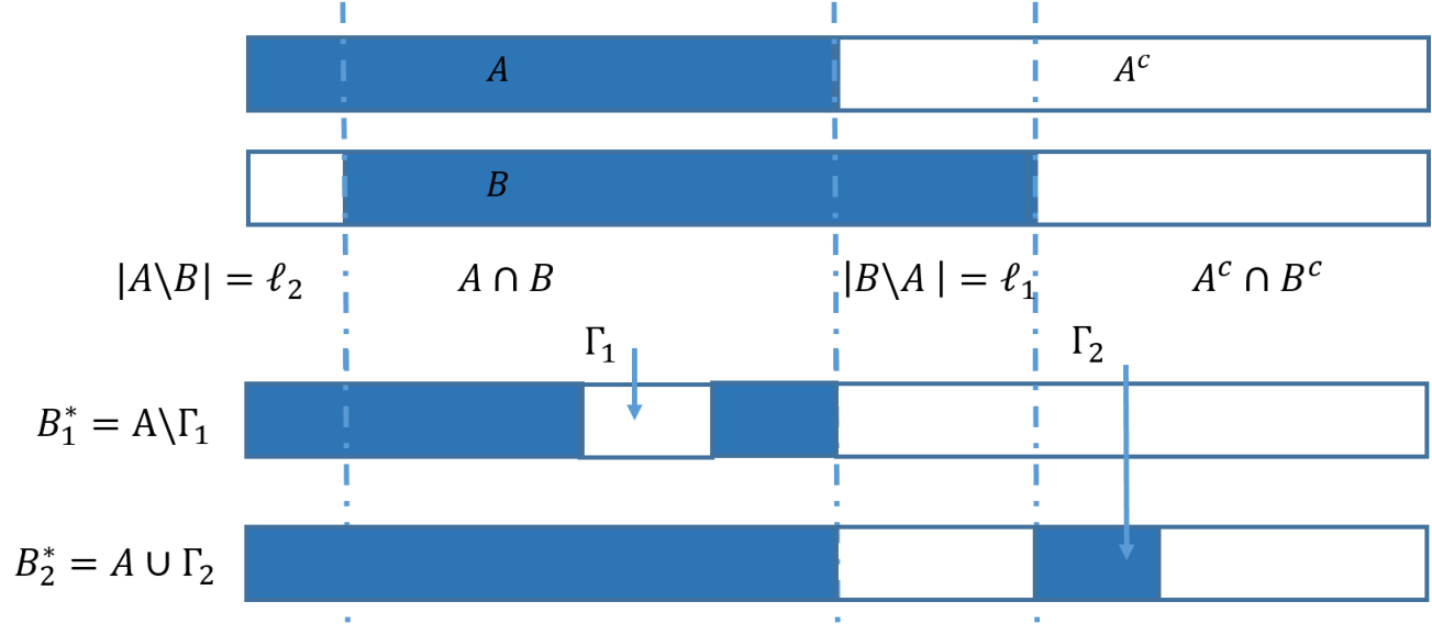
Refer to caption
Fig 9: The solid area are the streams with signal. The whole set [J][J] is partitioned into four disjoint sets: A∖BA\setminus B, A∩BA\cap B, B∖AB\setminus A, Ac∩BcA^{c}\cap B^{c}. If B∈𝒰k1,k2​(A)B\in\mathcal{U}_{k_{1},k_{2}}(A), then ℓ1<k1\ell_{1}<k_{1} and ℓ2<k2\ell_{2}<k_{2}.

C.4 Proof of Theorem 4.3

As explained in the discussion following Theorem 4.3, it suffices to show that for any A⊂[J]A\subset[J], as α,β→0\alpha,\beta\to 0,

NA∗​(k1,k2,α,β)≥LA​(k1,k2,α,β)​(1−o⁡(1)).N_{A}^{*}(k_{1},k_{2},\alpha,\beta)\geq L_{A}(k_{1},k_{2},\alpha,\beta)\,(1-o(1)).

Since k1,k2k_{1},k_{2} are fixed integers, in order to simplify the notation in this subsection we write

L⁡(A,α,β)​ for ​LA​(k1,k2,α,β).L(A;\alpha,\beta)\;\;\text{ for }\;\;L_{A}(k_{1},k_{2},\alpha,\beta).

Fix A⊂[J]A\subset[J]. By the same argument as in the proof of Theorem 3.2, it suffices to show for every q∈(0,1)q\in(0,1) we have:

lim infα,β→0inf(T,D)∈Δk1,k2​(α,β)𝖯A​(T≥q​L​(A,α,β))≥1.\displaystyle\liminf_{\alpha,\beta\to 0}\inf_{(T,D)\in\Delta_{k_{1},k_{2}}(\alpha,\beta)}{\sf P}_{A}\left(T\geq qL(A;\alpha,\beta)\right)\geq 1.

Fix q∈(0,1)q\in(0,1) and let (T,D)(T,D) be any procedure in Δk1,k2​(α,β)\Delta_{k_{1},k_{2}}(\alpha,\beta). Then, by the definition of the class 𝒰k1,k2​(A)\mathcal{U}_{k_{1},k_{2}}(A) in (53) we have

1−(α+β)≤𝖯A​(D∈𝒰k1,k2​(α,β))=∑B∈𝒰k1,k2​(α,β)𝖯A​(D=B).1-(\alpha+\beta)\leq{\sf P}_{A}\left(D\in\mathcal{U}_{k_{1},k_{2}}(\alpha,\beta)\right)=\sum_{B\in\mathcal{U}_{k_{1},k_{2}}(\alpha,\beta)}{\sf P}_{A}(D=B).

Fix B∈𝒰k1,k2​(α,β)B\in\mathcal{U}_{k_{1},k_{2}}(\alpha,\beta), and let η>0\eta>0. First, we assume that |B|≥k1|B|\geq k_{1} and |Bc|≥k2|B^{c}|\geq k_{2}. Then 𝖯A​(D=B){\sf P}_{A}(D=B) is upper bounded by I+II\text{I}+\text{II}, where

I=𝖯A​(λA,B1∗​(T)<log⁡(ηα),D=B)+𝖯A​(λA,B2∗​(T)<log⁡(ηβ),D=B)\displaystyle\text{I}={\sf P}_{A}\left(\lambda^{A,B_{1}^{*}}(T)<\log(\frac{\eta}{\alpha}),D=B\right)+{\sf P}_{A}\left(\lambda^{A,B_{2}^{*}}(T)<\log(\frac{\eta}{\beta}),D=B\right)
II=𝖯A​(λA,B1∗​(T)≥log⁡(ηα),λA,B2∗​(T)≥log⁡(ηβ),D=B),\displaystyle\text{II}={\sf P}_{A}\left(\lambda^{A,B_{1}^{*}}(T)\geq\log(\frac{\eta}{\alpha}),\lambda^{A,B_{2}^{*}}(T)\geq\log(\frac{\eta}{\beta}),D=B\right),

where the sets B1∗B_{1}^{*} and B2∗B_{2}^{*} are selected to satisfy the conditions in Case 1 of Lemma C.2. Then, |B∖B1∗|≥k1|B\setminus B_{1}^{*}|\geq k_{1} and |B2∗∖B|≥k2|B_{2}^{*}\setminus B|\geq k_{2}, and consequently

𝖯B1∗​(D=B)≤α​ and ​𝖯B2∗​(D=B)≤β.\displaystyle{\sf P}_{B_{1}^{*}}(D=B)\leq\alpha\;\text{ and }\;{\sf P}_{B_{2}^{*}}(D=B)\leq\beta.

Thus, by change of measure 𝖯A→𝖯B1∗{\sf P}_{A}\rightarrow{\sf P}_{B_{1}^{*}} and 𝖯A→𝖯B2∗{\sf P}_{A}\rightarrow{\sf P}_{B_{2}^{*}}, we have

𝖯A​(λA,Bi∗​(T)<log⁡(ηα),D=B)\displaystyle{\sf P}_{A}\left(\lambda^{A,B_{i}^{*}}(T)<\log\left(\frac{\eta}{\alpha}\right),D=B\right) ≤η, for i=1,2\displaystyle\leq\eta,\;\text{ for }\;i=1,2

which shows that I≤2​η\text{I}\leq 2\eta. Moreover, it is obvious that

II≤ϵα,βB​(T)+𝖯A​(T≥q​L​(A,α,β),D=B),where​ϵα,βB​(T):=\displaystyle\text{II}\leq\epsilon^{B}_{\alpha,\beta}(T)+{\sf P}_{A}(T\geq qL(A;\alpha,\beta),\;D=B),\quad\text{where}\epsilon^{B}_{\alpha,\beta}(T)\;:=
𝖯A​(T<q​L​(A,α,β),λA,B1∗​(T)≥log⁡(ηα),λA,B2∗​(T)≥log⁡(ηβ)).\displaystyle{\sf P}_{A}\left(T<qL(A;\alpha,\beta),\;\lambda^{A,B_{1}^{*}}(T)\geq\log\left(\frac{\eta}{\alpha}\right),\lambda^{A,B_{2}^{*}}(T)\geq\log\left(\frac{\eta}{\beta}\right)\right).

But by the construction of B1∗B_{1}^{*} and B2∗B_{2}^{*} we have

L⁡(A,α,β)≤ℓα,β:=|log⁡(α)|ℐA,B1∗​⋁|log⁡(β)|ℐA,B2∗,L(A;\alpha,\beta)\leq\ell_{\alpha,\beta}:=\frac{|\log(\alpha)|}{\mathcal{I}^{A,B_{1}^{*}}}\bigvee\frac{|\log(\beta)|}{\mathcal{I}^{A,B_{2}^{*}}},

consequently

ϵα,βB​(T)≤𝖯A​(T<q​ℓα,β,λA,B1∗​(T)≥log⁡(ηα),λA,B2∗​(T)≥log⁡(ηβ)),\displaystyle\epsilon^{B}_{\alpha,\beta}(T)\leq{\sf P}_{A}\left(T<q\ell_{\alpha,\beta},\;\;\lambda^{A,B_{1}^{*}}(T)\geq\log\left(\frac{\eta}{\alpha}\right),\lambda^{A,B_{2}^{*}}(T)\geq\log\left(\frac{\eta}{\beta}\right)\right),

and from Lemma F.1 it follows that ϵα,βB​(T)→0\epsilon^{B}_{\alpha,\beta}(T)\to 0 as α,β→0\alpha,\beta\to 0 uniformly in TT.

Putting everything together, we have

𝖯A​(D=B)≤2​η+ϵα,βB​(T)+𝖯A​(T≥q​L​(A,α,β),D=B).{\sf P}_{A}(D=B)\leq 2\eta+\epsilon^{B}_{\alpha,\beta}(T)+{\sf P}_{A}(T\geq qL(A;\alpha,\beta),D=B). (54)

In a similar way we can show that equation (54) remains valid when |B|<k1|B|<k_{1} or |Bc|<k2|B^{c}|<k_{2}. Thus summing over B∈𝒰k1,k2​(A)B\in\mathcal{U}_{k_{1},k_{2}}(A) we have

𝖯A​(D∈𝒰k1,k2​(A))\displaystyle{\sf P}_{A}(D\in\mathcal{U}_{k_{1},k_{2}}(A)) ≤2​Q​η+ϵα,β​(T)+𝖯A​(T≥q​L​(A,α,β),D∈𝒰k1,k2​(A)),\displaystyle\leq 2Q\eta+\epsilon_{\alpha,\beta}(T)+{\sf P}_{A}(T\geq qL(A;\alpha,\beta),D\in\mathcal{U}_{k_{1},k_{2}}(A)),

where Q=|𝒰k1,k2​(A)|Q=|\mathcal{U}_{k_{1},k_{2}}(A)| is a constant, and ϵα,β​(T)=∑B∈𝒰k1,k2​(A)ϵα,βB​(T).\epsilon_{\alpha,\beta}(T)=\sum_{B\in\mathcal{U}_{k_{1},k_{2}}(A)}\epsilon^{B}_{\alpha,\beta}(T). Since each summand goes to 00, we have ϵα,β​(T)→0\epsilon_{\alpha,\beta}(T)\to 0 as α,β→0\alpha,\beta\to 0 uniformly in TT. Therefore,

𝖯A​(T≥q​L​(A,α,β))≥1−(α+β)−2​Q​η−ϵα,β​(T)\displaystyle{\sf P}_{A}(T\geq qL(A;\alpha,\beta))\geq 1-(\alpha+\beta)-2Q\eta-\epsilon_{\alpha,\beta}(T)

The proof is complete after taking the infimum over the class Δk1,k2​(α,β)\Delta_{k_{1},k_{2}}(\alpha,\beta), letting α,β→0\alpha,\beta\to 0 and letting η→0\eta\to 0. ∎

C.5 Proof of Corollary 4.4

The error control for δ0\delta_{0} follows by setting ℓ=0\ell=0 in Lemma C.1. The error control for the Intersection rule δI\delta_{I} can be established by a simple modification of the proof of Lemma C.1. If assumptions (11) and (12) hold, then from (4.4) it follows that for every A⊂[J]A\subset[J] we have

LA​(k1,k1,α,α)=|log⁡(α)|k1​ℐ.\displaystyle L_{A}(k_{1},k_{1},\alpha,\alpha)=\frac{|\log(\alpha)|}{k_{1}\mathcal{I}}.

Further, setting ℓ=0\ell=0 for τ0\tau_{0}, and k=1k=1 for TIT_{I} in the first inequality of Lemma 4.2, we have as b→∞b\to\infty

𝖤A​[τ0​(b,b)]≤bk1​ℐ​(1+o⁡(1)),𝖤A​[τI​(b,b)]≤bℐ​(1+o⁡(1)).\displaystyle{\sf E}_{A}\left[\tau_{0}(b,b)\right]\;\leq\frac{b}{k_{1}\mathcal{I}}(1+o(1)),\quad{\sf E}_{A}\left[\tau_{I}(b,b)\right]\;\leq\frac{b}{\mathcal{I}}(1+o(1)).

Thus, if bb is selected as in the statement of the corollary, then the quantity LA​(k1,k1,α,α)L_{A}(k_{1},k_{1},\alpha,\alpha) provides an asymptotic power bound for both 𝖤A​[τ0]{\sf E}_{A}\left[\tau_{0}\right] and 𝖤A​[τI]{\sf E}_{A}\left[\tau_{I}\right]. Thus, the proof is complete. ∎

C.6 Proof of Theorem 4.5

Since k1,dk_{1},d are fixed, for simplicity we write n∗​(β)n^{*}(\beta) and n^​(β)\widehat{n}(\beta) for n∗​(k1,k1,βd,β)n^{*}(k_{1},k_{1},\beta^{d},\beta) and n^N​P​(k1,k1,βd,β)\widehat{n}_{NP}(k_{1},k_{1},\beta^{d},\beta), respectively.

(i) Let us first focus on n∗​(β)n^{*}(\beta). By its definition (13), there exists some

D∗​(β)∈Δf​i​x​(n∗​(β))∩Δk1,k1​(βd,β).D^{*}(\beta)\in\Delta_{fix}(n^{*}(\beta))\cap\Delta_{k_{1},k_{1}}(\beta^{d},\beta).

Fix any A⊂[J]A\subset[J] such that |A|=2​k1−1|A|=2k_{1}-1. Denote 𝖯{\sf P} the probability measure for data in all streams, and consider the simple versus simple testing problem (52) and the following procedure D~∗​(β):={0​ if ​|D∗​(β)|<k11​ if ​|D∗​(β)|≥k1.\widetilde{D}^{*}(\beta):=\begin{cases}0\;\;\text{ if }|D^{*}(\beta)|<k_{1}\\ 1\;\;\text{ if }|D^{*}(\beta)|\geq k_{1}.\end{cases} Then, by definition of D∗​(β)D^{*}(\beta) we have

𝖯∅​(D~∗​(β)=1)=𝖯∅​(|D∗​(β)|≥k1)≤α=βd,\displaystyle{\sf P}_{\emptyset}(\widetilde{D}^{*}(\beta)=1)={\sf P}_{\emptyset}(|D^{*}(\beta)|\geq k_{1})\leq\alpha=\beta^{d},
𝖯A​(D~∗​(β)=0)=𝖯A​(|D∗​(β)|<k1)≤β,\displaystyle{\sf P}_{A}(\widetilde{D}^{*}(\beta)=0)={\sf P}_{A}(|D^{*}(\beta)|<k_{1})\leq\beta,

and by the generalized Chernoff’s Lemma G.1,

lim infβ→0log⁡(β)n∗​(β)\displaystyle\liminf_{\beta\to 0}\frac{\log(\beta)}{n^{*}(\beta)} ≥lim infβ→01n∗​(β)​log⁡(12​𝖯∅1/d​(D~∗​(β)=1)+12​𝖯A​(D~∗​(β)=0))\displaystyle\geq\liminf_{\beta\to 0}\frac{1}{n^{*}(\beta)}\log\left(\frac{1}{2}{\sf P}_{\emptyset}^{1/d}(\widetilde{D}^{*}(\beta)=1)+\frac{1}{2}{\sf P}_{A}(\widetilde{D}^{*}(\beta)=0)\right)
≥−ΦA​(h~dA)d.\displaystyle\geq-\frac{\Phi^{A}(\widetilde{h}_{d}^{A})}{d}.

where h~dA\widetilde{h}_{d}^{A} is a solution to ΦA​(z)/d=ΦA​(z)−z\Phi^{A}(z)/d=\Phi^{A}(z)-z, and for any z∈ℝz\in{\mathbb{R}}

ΦA​(z)\displaystyle\Phi^{A}(z) :=supθ∈ℝ{z​θ−∑j∈Alog⁡(𝖤0j​[eθ​λj​(1)])}\displaystyle:=\sup_{\theta\in{\mathbb{R}}}\left\{z\theta-\sum_{j\in A}\log\left({\sf E}_{0}^{j}\left[e^{\theta\lambda^{j}(1)}\right]\right)\right\}
=supθ∈ℝ{z​θ−|A|​log⁡(𝖤01​[eθ​λ1​(1)])}=|A|​Φ​(z/|A|).\displaystyle=\sup_{\theta\in{\mathbb{R}}}\left\{z\theta-|A|\log\left({\sf E}_{0}^{1}\left[e^{\theta\lambda^{1}(1)}\right]\right)\right\}=|A|\,\Phi(z/|A|).

Here, the second equality is due to homogeneity (34). By definition (36), Φ⁡(hd)/d=Φ⁡(hd)−hd{\Phi({h}_{d})}/{d}=\Phi({h}_{d})-{h}_{d}, which implies

ΦA​(|A|​hd)/d=ΦA​(|A|​hd)−(|A|​hd).{\Phi^{A}(|A|{h}_{d})}/{d}=\Phi^{A}(|A|{h}_{d})-(|A|{h}_{d}).

Thus, h~dA=|A|​hd\widetilde{h}_{d}^{A}=|A|{h}_{d}, and

ΦA​(h~dA)/d=|A|​Φ​(hd)/d=2​k1−1d​Φ​(hd),{\Phi^{A}(\widetilde{h}_{d}^{A})}/{d}=|A|\Phi({h}_{d})/{d}=\frac{2k_{1}-1}{d}\Phi({h}_{d}),

which completes the proof of (i).

(ii) We now focus on n^​(β)\widehat{n}(\beta). By definition, there exists hβ∈ℝh_{\beta}\in{\mathbb{R}} such that

(n^​(β),D^​(β))∈Δk1,k1​(βd,β), where ​D^​(β):=DN​P​(n^​(β),hβ​𝟏J),(\widehat{n}(\beta),\widehat{D}(\beta))\in\Delta_{k_{1},k_{1}}(\beta^{d},\beta),\text{ where }\widehat{D}(\beta):=D_{NP}(\widehat{n}(\beta),h_{\beta}\mathbf{1}_{J}),

where 𝟏J∈ℝJ\mathbf{1}_{J}\in{\mathbb{R}}^{J} is a vector of all ones. Due to homogeneity (34), set

pβ:=𝖯01​(D^1​(β)=1)=𝖯01​(λ1​(n^​(β))>hβ​n^​(β)),\displaystyle p_{\beta}:={\sf P}_{0}^{1}(\widehat{D}^{1}(\beta)=1)={\sf P}_{0}^{1}\left(\lambda^{1}(\widehat{n}(\beta))>h_{\beta}\,\widehat{n}(\beta)\right),
qβ:=𝖯11​(D^1​(β)=0)=𝖯11​(λ1​(n^​(β))≤hβ​n^​(β)).\displaystyle q_{\beta}:={\sf P}_{1}^{1}(\widehat{D}^{1}(\beta)=0)={\sf P}_{1}^{1}\left(\lambda^{1}(\widehat{n}(\beta))\leq h_{\beta}\,\widehat{n}(\beta)\right).

For any A⊂[J]A\subset[J] such that |A|=k1(=k2)|A|=k_{1}(=k_{2}),

βd\displaystyle\beta^{d} ≥𝖯∅(⋂j∈A{D~(α)j=1})=(pβ)k1,\displaystyle\geq{\sf P}_{\emptyset}\left(\bigcap_{j\in A}\{\tilde{D}(\alpha)^{j}=1\}\right)=(p_{\beta})^{k_{1}},\;\;
β\displaystyle\beta ≥𝖯[J](⋂j∈A{D~(α)j=0})=(qβ)k1,\displaystyle\geq{\sf P}_{[J]}\left(\bigcap_{j\in A}\{\tilde{D}(\alpha)^{j}=0\}\right)=(q_{\beta})^{k_{1}},

which implies that

1n^​(β)​log⁡(β)k1≥1n^​(β)​log⁡(12​pβ1/d+12​qβ).\displaystyle\frac{1}{\widehat{n}(\beta)}\frac{\log(\beta)}{k_{1}}\geq\frac{1}{\widehat{n}(\beta)}\log\left(\frac{1}{2}p_{\beta}^{1/d}+\frac{1}{2}q_{\beta}\right).

Then, again by the generalized Chernoff’s lemma G.1 we have

liminfβ→0n^​(β)|log⁡(β)|=dk1​Φ​(hd).\displaystyle\lim\inf_{\beta\to 0}\frac{\widehat{n}(\beta)}{|\log(\beta)|}=\frac{d}{k_{1}\Phi({h}_{d})}.

Further, the same argument shows that the equality is obtained with h=hdh={h}_{d}, which completes the proof of (ii). ∎

D Sequential multiple testing with composite hypotheses

In this section, we prove Theorem 6.1 in Section 6. We first establish a universal asymptotic lower bound on the expected sample size of procedures that control generalized familywise error rates under composite hypotheses (Subsec. D.1). Then, we show that this lower bound is achieved by the Leap rule with the adaptive log-likelihood statistics in (38) (Subsec. D.2 and D.3). Further, we demonstrate numerically that the Intersection rule (10) and the asymmetric Sum-Intersection rule (23) with the adaptive statistics fail to achieve asymptotic optimality in the composite case (Subsec. D.4). We conclude this section with a discussion on the adaptive statistics and alternative local test statistics (Subsec. D.5).

D.1 Lower bound on the expected sample size

Fix any A⊂[J]A\subset[J] and 𝛉=(θ1,…,θJ)∈𝚯A\boldsymbol{\uptheta}=(\theta^{1},\ldots,\theta^{J})\in\boldsymbol{\Theta}_{A}.

Case 1: Assume for now that the infima in (40) are attained, i.e., there exists 𝛉~=(θ~1,…,θ~J)∈𝚯Ac\widetilde{\boldsymbol{\uptheta}}=(\widetilde{\theta}^{1},\ldots,\widetilde{\theta}^{J})\in\boldsymbol{\Theta}_{A^{c}} such that

ℐ0j​(θj)=Ij​(θj,θ~j)​ for every ​j∈Ac,\displaystyle\mathcal{I}_{0}^{j}(\theta^{j})=I^{j}(\theta^{j},\widetilde{\theta}^{j})\text{ for every }j\in A^{c},
ℐ1j​(θj)=Ij​(θj,θ~j)​ for every ​j∈A.\displaystyle\mathcal{I}_{1}^{j}(\theta^{j})=I^{j}(\theta^{j},\widetilde{\theta}^{j})\text{ for every }j\in A.

Any procedure (T,D)∈Δk1,k2c​o​m​p​(α,β)(T,D)\in\Delta_{k_{1},k_{2}}^{comp}(\alpha,\beta) controls the generalized familywise error rates below α\alpha and β\beta when applied to the multiple testing problem with the following simple hypotheses for each stream:

𝖧0j:γj=θj​ versus ​𝖧1j:γj=θ~j,j∈Ac,\displaystyle{\sf{H}}_{0}^{j}\;:\gamma^{j}=\theta^{j}\;\;\text{ versus }\;\;{\sf{H}}_{1}^{j}\;:\gamma^{j}=\widetilde{\theta}^{j},\quad j\in A^{c},
𝖧0j:γj=θ~j​ versus ​𝖧1j:γj=θj,j∈A,\displaystyle{\sf{H}}_{0}^{j}\;:\gamma^{j}=\widetilde{\theta}^{j}\;\;\text{ versus }\;\;{\sf{H}}_{1}^{j}\;:\gamma^{j}=\theta^{j},\quad j\in A,

where we write γj\gamma^{j} for the generic local parameter in j-th stream to distinguish it from the j-th component of 𝛉\boldsymbol{\uptheta}.

Then, under assumptions (39) and (41), by Theorem 4.3 we have

lim infα,β→0NA,𝛉∗​(k1,k2,α,β)/LA,𝛉​(k1,k2,α,β)≥1,\displaystyle\liminf_{\alpha,\beta\to 0}\;N^{*}_{A,\boldsymbol{\uptheta}}(k_{1},k_{2},\alpha,\beta)/L_{A,\boldsymbol{\uptheta}}(k_{1},k_{2},\alpha,\beta)\geq 1, (55)

where

LA,𝛉​(k1,k2,α,β):=min⁡{min0≤ℓ<k1⁡L^A,𝛉​(ℓ,α,β),min0≤ℓ<k2⁡ ^LA,𝛉​(ℓ,α,β)},L^A,𝛉​(ℓ,α,β):=max⁡{|log⁡(α)|𝒟1​(A,𝛉,1,k1−ℓ),|log⁡(β)|𝒟0​(Ac,𝛉,ℓ+1,ℓ+k2)}, ^LA,𝛉​(ℓ,α,β):=max⁡{|log⁡(α)|𝒟1​(A,𝛉,ℓ+1,ℓ+k1),|log⁡(β)|𝒟0​(Ac,𝛉,1,k2−ℓ)},𝒟1(A,𝛉;ℓ,u)=∑j=ℓuℐ(j)1(A,𝛉),𝒟0(Ac,𝛉;ℓ,u)=∑j=ℓuℐ(j)0(Ac,𝛉),\displaystyle\begin{split}&L_{A,\boldsymbol{\uptheta}}(k_{1},k_{2},\alpha,\beta):=\min\left\{\min_{0\leq\ell<k_{1}}\widehat{L}_{A,\boldsymbol{\uptheta}}(\ell;\alpha,\beta)\;,\;\min_{0\leq\ell<k_{2}}{\mathchoice{{\vtop{\halign{#\cr\hbox{\raise 7.09259pt\hbox{\scalebox{1}[-1]{\lower 7.09259pt\hbox{$\displaystyle\widehat{\vrule width=0.0pt,height=6.83331pt\vrule height=0.0pt,width=6.80557pt}$}}}}\cr\hbox{$\displaystyle L$}\crcr}}}}{{\vtop{\halign{#\cr\hbox{\raise 7.09259pt\hbox{\scalebox{1}[-1]{\lower 7.09259pt\hbox{$\textstyle\widehat{\vrule width=0.0pt,height=6.83331pt\vrule height=0.0pt,width=6.80557pt}$}}}}\cr\hbox{$\textstyle L$}\crcr}}}}{{\vtop{\halign{#\cr\hbox{\raise 6.40926pt\hbox{\scalebox{1}[-1]{\lower 6.40926pt\hbox{$\scriptstyle\widehat{\vrule width=0.0pt,height=4.78334pt\vrule height=0.0pt,width=5.48615pt}$}}}}\cr\hbox{$\scriptstyle L$}\crcr}}}}{{\vtop{\halign{#\cr\hbox{\raise 5.9537pt\hbox{\scalebox{1}[-1]{\lower 5.9537pt\hbox{$\scriptscriptstyle\widehat{\vrule width=0.0pt,height=3.41667pt\vrule height=0.0pt,width=4.77783pt}$}}}}\cr\hbox{$\scriptscriptstyle L$}\crcr}}}}}_{A,\boldsymbol{\uptheta}}(\ell;\alpha,\beta)\right\},\\ &\widehat{L}_{A,\boldsymbol{\uptheta}}(\ell;\alpha,\beta):=\max\left\{\frac{|\log(\alpha)|}{\mathcal{D}_{1}(A,\boldsymbol{\uptheta};1,k_{1}-\ell)}\;,\;\frac{|\log(\beta)|}{\mathcal{D}_{0}(A^{c},\boldsymbol{\uptheta};\ell+1,\ell+k_{2})}\right\},\\ &{\mathchoice{{\vtop{\halign{#\cr\hbox{\raise 7.09259pt\hbox{\scalebox{1}[-1]{\lower 7.09259pt\hbox{$\displaystyle\widehat{\vrule width=0.0pt,height=6.83331pt\vrule height=0.0pt,width=6.80557pt}$}}}}\cr\hbox{$\displaystyle L$}\crcr}}}}{{\vtop{\halign{#\cr\hbox{\raise 7.09259pt\hbox{\scalebox{1}[-1]{\lower 7.09259pt\hbox{$\textstyle\widehat{\vrule width=0.0pt,height=6.83331pt\vrule height=0.0pt,width=6.80557pt}$}}}}\cr\hbox{$\textstyle L$}\crcr}}}}{{\vtop{\halign{#\cr\hbox{\raise 6.40926pt\hbox{\scalebox{1}[-1]{\lower 6.40926pt\hbox{$\scriptstyle\widehat{\vrule width=0.0pt,height=4.78334pt\vrule height=0.0pt,width=5.48615pt}$}}}}\cr\hbox{$\scriptstyle L$}\crcr}}}}{{\vtop{\halign{#\cr\hbox{\raise 5.9537pt\hbox{\scalebox{1}[-1]{\lower 5.9537pt\hbox{$\scriptscriptstyle\widehat{\vrule width=0.0pt,height=3.41667pt\vrule height=0.0pt,width=4.77783pt}$}}}}\cr\hbox{$\scriptscriptstyle L$}\crcr}}}}}_{A,\boldsymbol{\uptheta}}(\ell;\alpha,\beta):=\max\left\{\frac{|\log(\alpha)|}{\mathcal{D}_{1}(A,\boldsymbol{\uptheta};\ell+1,\ell+k_{1})}\;,\;\frac{|\log(\beta)|}{\mathcal{D}_{0}(A^{c},\boldsymbol{\uptheta};1,k_{2}-\ell)}\right\},\\ &\mathcal{D}_{1}(A,\boldsymbol{\uptheta};\ell,u)=\sum_{j=\ell}^{u}\mathcal{I}^{(j)}_{1}(A,\boldsymbol{\uptheta}),\quad\mathcal{D}_{0}(A^{c},\boldsymbol{\uptheta};\ell,u)=\sum_{j=\ell}^{u}\mathcal{I}^{(j)}_{0}(A^{c},\boldsymbol{\uptheta}),\end{split} (56)

and

ℐ1(1)​(A,𝛉)≤…≤ℐ1(|A|)​(A,𝛉)\mathcal{I}^{(1)}_{1}(A,\boldsymbol{\uptheta})\leq\ldots\leq\mathcal{I}^{(|A|)}_{1}(A,\boldsymbol{\uptheta})

is the increasingly ordered sequence of {ℐ1j​(θj),j∈A}\{\mathcal{I}_{1}^{j}(\theta^{j}),j\in A\}, and

ℐ0(1)​(Ac,𝛉)≤…≤ℐ0(|Ac|)​(Ac,𝛉)\mathcal{I}^{(1)}_{0}(A^{c},\boldsymbol{\uptheta})\leq\ldots\leq\mathcal{I}^{(|A^{c}|)}_{0}(A^{c},\boldsymbol{\uptheta})

is the increasingly ordered sequence of {ℐ0j​(θj),j∈Ac}\{\mathcal{I}_{0}^{j}(\theta^{j}),j\in A^{c}\}. As before, the convention is that

ℐ1(j)​(A,𝛉)=∞​ if ​j>|A|,ℐ0(j)​(Ac,𝛉)=∞​ if ​j>|Ac|.\mathcal{I}^{(j)}_{1}(A,\boldsymbol{\uptheta})=\infty\;\text{ if }j>|A|,\quad\mathcal{I}^{(j)}_{0}(A^{c},\boldsymbol{\uptheta})=\infty\;\text{ if }j>|A^{c}|.

Case 2: In general, the infima in (40) are not attained. However, under the separability assumption (41), for any ϵ>0\epsilon>0 there exists 𝛉~ϵ=(θ~ϵ1,…,θ~ϵJ)∈𝚯Ac\widetilde{\boldsymbol{\uptheta}}_{\epsilon}=(\widetilde{\theta}^{1}_{\epsilon},\ldots,\widetilde{\theta}^{J}_{\epsilon})\in\boldsymbol{\Theta}_{A^{c}} such that

Ij​(θj,θ~ϵj)≤(1+ϵ)​ℐ0j​(θj)​ for any ​j∈Ac,\displaystyle I^{j}(\theta^{j},\widetilde{\theta}_{\epsilon}^{j})\leq(1+\epsilon)\,\mathcal{I}_{0}^{j}(\theta^{j})\text{ for any }j\in A^{c},
Ij​(θj,θ~ϵj)≤(1+ϵ)​ℐ1j​(θj)​ for any ​j∈A.\displaystyle I^{j}(\theta^{j},\widetilde{\theta}_{\epsilon}^{j})\leq(1+\epsilon)\,\mathcal{I}_{1}^{j}(\theta^{j})\text{ for any }j\in A.

Applying again Theorem 4.3 to the following multiple testing problem with simple hypotheses:

𝖧0j:γj=θj​ versus ​𝖧1j:γj=θ~ϵj,j∈Ac,\displaystyle{\sf{H}}_{0}^{j}\;:\gamma^{j}=\theta^{j}\;\;\text{ versus }\;\;{\sf{H}}_{1}^{j}\;:\gamma^{j}=\widetilde{\theta}_{\epsilon}^{j},\quad j\in A^{c},
𝖧0j:γj=θ~ϵj​ versus ​𝖧1j:γj=θj,j∈A,\displaystyle{\sf{H}}_{0}^{j}\;:\gamma^{j}=\widetilde{\theta}_{\epsilon}^{j}\;\;\text{ versus }\;\;{\sf{H}}_{1}^{j}\;:\gamma^{j}=\theta^{j},\quad j\in A,

we have

lim infNA,𝛉∗​(k1,k2,α,β)/LA,𝛉​(k1,k2,α,β)≥1/(1+ϵ).\liminf\;N^{*}_{A,\boldsymbol{\uptheta}}(k_{1},k_{2},\alpha,\beta)/L_{A,\boldsymbol{\uptheta}}(k_{1},k_{2},\alpha,\beta)\geq 1/(1+\epsilon).

Since ϵ\epsilon is arbitrary, (55) still holds.

Above discussions leads to the following theorem.

Theorem D.1.

If (39) and (41) hold, then (55) holds for every A⊂[J]A\subset[J] and 𝛉∈𝚯A\boldsymbol{\uptheta}\in\boldsymbol{\Theta}_{A}.

D.2 Error control of the Leap rule with adaptive log-likelihood ratios

We start with the following observation.

Lemma D.2.

Fix A⊂[J]A\subset[J], 𝛉=(θ1,…,θJ)∈ΘA\boldsymbol{\uptheta}=(\theta^{1},\ldots,\theta^{J})\in\Theta_{A}. For each j∈[J]j\in[J],

Lnj:=exp⁡(ℓ∗j​(n)−ℓj​(n,θj)),n∈ℕL_{n}^{j}:=\exp\left({\ell}^{j}_{*}(n)-\ell^{j}(n,\theta^{j})\right),\;\;n\in\mathbb{N}

is an {ℱn}\{\mathcal{F}_{n}\}-martingale under 𝖯A,𝛉{\sf P}_{A,\boldsymbol{\uptheta}} with expectation 11.

By definition,

Lnj=Ln−1j⋅pθ^n−1jj​(Xj​(n)|ℱn−1j)pθjj​(Xj​(n)|ℱn−1j).\displaystyle L_{n}^{j}=L^{j}_{n-1}\cdot\frac{p^{j}_{\widehat{\theta}_{n-1}^{j}}\left(X^{j}(n)|\mathcal{F}^{j}_{n-1}\right)}{p^{j}_{\theta^{j}}\left(X^{j}(n)|\mathcal{F}^{j}_{n-1}\right)}\;\;.

Clearly, Lnj∈ℱnL_{n}^{j}\in\mathcal{F}_{n} for any n∈ℕn\in\mathbb{N}. Further, since θ^n−1j∈ℱn−1\widehat{\theta}_{n-1}^{j}\in\mathcal{F}_{n-1},

𝖤A,𝛉[pθ^n−1jj​(Xj​(n)|ℱn−1j)pθjj​(Xj​(n)|ℱn−1j)|ℱn−1]=∫pθ^n−1jj​(z|ℱn−1j)pθjj​(z|ℱn−1j)pθjj(z|ℱn−1j)=1,\displaystyle{\sf E}_{A,\boldsymbol{\uptheta}}\left[\left.\frac{p^{j}_{\widehat{\theta}_{n-1}^{j}}\left(X^{j}(n)|\mathcal{F}^{j}_{n-1}\right)}{p^{j}_{\theta^{j}}\left(X^{j}(n)|\mathcal{F}^{j}_{n-1}\right)}\right|\mathcal{F}_{n-1}\right]=\int\,\frac{p^{j}_{\widehat{\theta}_{n-1}^{j}}\left(z|\mathcal{F}^{j}_{n-1}\right)}{p^{j}_{\theta^{j}}\left(z|\mathcal{F}^{j}_{n-1}\right)}p^{j}_{\theta^{j}}\left(z|\mathcal{F}^{j}_{n-1}\right)=1,

which implies 𝖤A,𝛉​[Lnj|ℱn−1]=Ln−1j{\sf E}_{A,\boldsymbol{\uptheta}}[L^{j}_{n}|\mathcal{F}_{n-1}]=L^{j}_{n-1}. Further, since 𝛉^0\widehat{\boldsymbol{\uptheta}}_{0} is deterministic, 𝖤A,𝛉​[L1j]=1{\sf E}_{A,\boldsymbol{\uptheta}}[L^{j}_{1}]=1, which completes the proof. ∎

By Lemma D.2 and due to independence across streams, for any subset M⊂[J]M\subset[J], there exists a probability measure QA,𝛉,MQ_{A,\boldsymbol{\uptheta},M} such that for any n∈ℕn\in\mathbb{N},

d​QA,𝛉,Md​𝖯A,𝛉​(ℱn)=∏j∈Mexp⁡(ℓ∗j​(n)−ℓj​(n,θj)).\frac{dQ_{A,\boldsymbol{\uptheta},M}}{d{\sf P}_{A,\boldsymbol{\uptheta}}}(\mathcal{F}_{n})\;=\;\prod_{j\in M}\exp\left({\ell}^{j}_{*}(n)-\ell^{j}(n,\theta^{j})\right). (57)

Next, we establish the error control of the Leap rule with adaptive log-likelihood ratios. The proof is almost identical to Theorem 4.1.

Theorem D.3.

Assume (40) and (41) hold. For any α,β∈(0,1)\alpha,\beta\in(0,1) we have that the Leap rule δL∗​(a,b)∈Δk1,k2c​o​m​p​(α,β)\delta_{L}^{*}(a,b)\in\Delta_{k_{1},k_{2}}^{comp}(\alpha,\beta) when the thresholds are selected as follows:

a=|log⁡(β)|+log⁡(2k2​Ck2J),b=|log⁡(α)|+log⁡(2k1​Ck1J).a=|\log(\beta)|+\log(2^{k_{2}}C^{J}_{k_{2}}),\quad b=|\log(\alpha)|+\log(2^{k_{1}}C^{J}_{k_{1}}).

Just as Theorem 4.1 follows from Lemma C.1 (see the proof in Appendix C.1), in the same way Theorem D.3 follows by the next Lemma. ∎

Lemma D.4.

Assume (40), (41) hold. Fix A⊂[J]A\subset[J], 𝛉=(θ1,…,θJ)∈𝚯A\boldsymbol{\uptheta}=(\theta^{1},\ldots,\theta^{J})\in\boldsymbol{\Theta}_{A}. Let B1⊂AcB_{1}\subset A^{c} with |B1|=k1|B_{1}|=k_{1}, and B2⊂AB_{2}\subset A with |B2|=k2|B_{2}|=k_{2}.

  1. (i)

    Fix any 0≤ℓ<k10\leq\ell<k_{1}. For any event Γ∈ℱτ^ℓ\Gamma\in\mathcal{F}_{\widehat{\tau}_{\ell}}, we have

    𝖯A,𝛉​(B1⊂D^ℓ∗)≤Cℓk1​e−b,𝖯A,𝛉​(B2⊂(D^ℓ∗)c,Γ)≤e−a​QA,𝛉,B2​(Γ).{\sf P}_{A,\boldsymbol{\uptheta}}(B_{1}\subset\widehat{D}^{*}_{\ell})\leq C_{\ell}^{k_{1}}e^{-b},\quad{\sf P}_{A,\boldsymbol{\uptheta}}(B_{2}\subset(\widehat{D}^{*}_{\ell})^{c},\,\Gamma)\leq e^{-a}Q_{A,\boldsymbol{\uptheta},B_{2}}(\Gamma).
  2. (ii)

    Fix any 0≤ℓ<k20\leq\ell<k_{2}. For any event Γ∈ℱ
     

     ^

     
    τ
    ℓ
    \Gamma\in\mathcal{F}_{{\mathchoice{{\vtop{\halign{#\cr\hbox{\raise 5.81944pt\hbox{\scalebox{1}[-1]{\lower 5.81944pt\hbox{$\displaystyle\widehat{\vrule width=0.0pt,height=3.01389pt\vrule height=0.0pt,width=3.68787pt}$}}}}\cr\hbox{$\displaystyle\tau$}\crcr}}}}{{\vtop{\halign{#\cr\hbox{\raise 5.81944pt\hbox{\scalebox{1}[-1]{\lower 5.81944pt\hbox{$\textstyle\widehat{\vrule width=0.0pt,height=3.01389pt\vrule height=0.0pt,width=3.68787pt}$}}}}\cr\hbox{$\textstyle\tau$}\crcr}}}}{{\vtop{\halign{#\cr\hbox{\raise 5.51805pt\hbox{\scalebox{1}[-1]{\lower 5.51805pt\hbox{$\scriptstyle\widehat{\vrule width=0.0pt,height=2.10971pt\vrule height=0.0pt,width=2.14204pt}$}}}}\cr\hbox{$\scriptstyle\tau$}\crcr}}}}{{\vtop{\halign{#\cr\hbox{\raise 5.31712pt\hbox{\scalebox{1}[-1]{\lower 5.31712pt\hbox{$\scriptscriptstyle\widehat{\vrule width=0.0pt,height=1.50694pt\vrule height=0.0pt,width=1.53003pt}$}}}}\cr\hbox{$\scriptscriptstyle\tau$}\crcr}}}}}_{\ell}}
    , we have

    𝖯A,𝛉​(B1⊂
     

     ^

     
    D
    ℓ∗
    ,Γ)
    ≤e−b​QA,𝛉,B1​(Γ)
    ,𝖯A,𝛉​(B2⊂(
     

     ^

     
    D
    ℓ∗
    )
    c
    )
    ≤Cℓk2​e−a
    .
    {\sf P}_{A,\boldsymbol{\uptheta}}(B_{1}\subset{\mathchoice{{\vtop{\halign{#\cr\hbox{\raise 7.09259pt\hbox{\scalebox{1}[-1]{\lower 7.09259pt\hbox{$\displaystyle\widehat{\vrule width=0.0pt,height=6.83331pt\vrule height=0.0pt,width=8.55695pt}$}}}}\cr\hbox{$\displaystyle D$}\crcr}}}}{{\vtop{\halign{#\cr\hbox{\raise 7.09259pt\hbox{\scalebox{1}[-1]{\lower 7.09259pt\hbox{$\textstyle\widehat{\vrule width=0.0pt,height=6.83331pt\vrule height=0.0pt,width=8.55695pt}$}}}}\cr\hbox{$\textstyle D$}\crcr}}}}{{\vtop{\halign{#\cr\hbox{\raise 6.40926pt\hbox{\scalebox{1}[-1]{\lower 6.40926pt\hbox{$\scriptstyle\widehat{\vrule width=0.0pt,height=4.78334pt\vrule height=0.0pt,width=6.75377pt}$}}}}\cr\hbox{$\scriptstyle D$}\crcr}}}}{{\vtop{\halign{#\cr\hbox{\raise 5.9537pt\hbox{\scalebox{1}[-1]{\lower 5.9537pt\hbox{$\scriptscriptstyle\widehat{\vrule width=0.0pt,height=3.41667pt\vrule height=0.0pt,width=5.72299pt}$}}}}\cr\hbox{$\scriptscriptstyle D$}\crcr}}}}}^{*}_{\ell},\,\Gamma)\leq e^{-b}Q_{A,\boldsymbol{\uptheta},B_{1}}(\Gamma),\quad{\sf P}_{A,\boldsymbol{\uptheta}}(B_{2}\subset({\mathchoice{{\vtop{\halign{#\cr\hbox{\raise 7.09259pt\hbox{\scalebox{1}[-1]{\lower 7.09259pt\hbox{$\displaystyle\widehat{\vrule width=0.0pt,height=6.83331pt\vrule height=0.0pt,width=8.55695pt}$}}}}\cr\hbox{$\displaystyle D$}\crcr}}}}{{\vtop{\halign{#\cr\hbox{\raise 7.09259pt\hbox{\scalebox{1}[-1]{\lower 7.09259pt\hbox{$\textstyle\widehat{\vrule width=0.0pt,height=6.83331pt\vrule height=0.0pt,width=8.55695pt}$}}}}\cr\hbox{$\textstyle D$}\crcr}}}}{{\vtop{\halign{#\cr\hbox{\raise 6.40926pt\hbox{\scalebox{1}[-1]{\lower 6.40926pt\hbox{$\scriptstyle\widehat{\vrule width=0.0pt,height=4.78334pt\vrule height=0.0pt,width=6.75377pt}$}}}}\cr\hbox{$\scriptstyle D$}\crcr}}}}{{\vtop{\halign{#\cr\hbox{\raise 5.9537pt\hbox{\scalebox{1}[-1]{\lower 5.9537pt\hbox{$\scriptscriptstyle\widehat{\vrule width=0.0pt,height=3.41667pt\vrule height=0.0pt,width=5.72299pt}$}}}}\cr\hbox{$\scriptscriptstyle D$}\crcr}}}}}^{*}_{\ell})^{c})\leq C_{\ell}^{k_{2}}e^{-a}.

The proof is similar to that of Lemma C.1. We only indicate the differences by working out the first inequality in (i).

As in the proof of Lemma C.1, by definition, D^ℓ∗\widehat{D}^{*}_{\ell} rejects the nulls in the ℓ\ell streams with the least significant non-positive LLR, in addition to the nulls in the streams with positive LLR. Thus,

{B1⊂D^ℓ∗}⊂⋃M⊂B1,|M|=k1−ℓΠM, where ΠM:={λ∗j(τ^ℓ)>0∀j∈M},\{B_{1}\subset\widehat{D}^{*}_{\ell}\}\subset\bigcup_{M\subset B_{1},|M|=k_{1}-\ell}\Pi_{M}\;,\quad\text{ where }\;\Pi_{M}:=\{\lambda^{j}_{*}(\widehat{\tau}_{\ell})>0\;\;\forall j\;\in M\},

and by Boole’s inequality it suffices to show that 𝖯A,𝛉​(ΠM)≤e−b{\sf P}_{A,\boldsymbol{\uptheta}}(\Pi_{M})\leq e^{-b} for every M⊂B1M\subset B_{1} with |M|=k1−ℓ|M|=k_{1}-\ell.

By definition, for any j∈M⊂B1⊂Acj\in M\subset B_{1}\subset A^{c}, since θj∈Θ0j\theta^{j}\in\Theta^{j}_{0},

ℓ0j​(n)≥ℓj​(n,θj)​ for any ​n∈ℕ.{\ell}^{j}_{0}(n)\geq\ell^{j}(n,\theta^{j})\;\;\text{ for any }n\in\mathbb{N}.

Then, by the definition of the adaptive log-likelihood ratio statistics (38), we have

ΠM⊂{∑j∈M(ℓ∗j(τ^ℓ)−ℓ0j(τ^ℓ))≥b}⊂{∑j∈M(ℓ∗j(τ^ℓ)−ℓj(τ^ℓ,θj))≥b}.\Pi_{M}\;\subset\;\left\{\sum_{j\in M}\left({\ell}^{j}_{*}(\widehat{\tau}_{\ell})-{\ell}^{j}_{0}(\widehat{\tau}_{\ell})\right)\geq b\right\}\;\subset\;\left\{\sum_{j\in M}\left({\ell}^{j}_{*}(\widehat{\tau}_{\ell})-\ell^{j}(\widehat{\tau}_{\ell},\theta^{j})\right)\geq b\right\}.

By the above observation, the definition of QA,𝛉,MQ_{A,\boldsymbol{\uptheta},M} (57), and likelihood ratio identity, on the event ΠM\Pi_{M},

d​QA,𝛉,Md​𝖯A,𝛉​(ℱτ^ℓ)≥eb,\frac{dQ_{A,\boldsymbol{\uptheta},M}}{d{\sf P}_{A,\boldsymbol{\uptheta}}}(\mathcal{F}_{\widehat{\tau}_{\ell}})\geq e^{b},

and the proof is complete by changing the measure from 𝖯A,𝛉{\sf P}_{A,\boldsymbol{\uptheta}} to QA,𝛉,MQ_{A,\boldsymbol{\uptheta},M}. ∎

D.3 Asymptotic optimality of the Leap rule with adaptive log-likelihood ratios

The asymptotic optimality follows after we establish an asymptotic upper bound on the expected sample size of the Leap rule. The following result is similar to Lemma 4.2.

Lemma D.5.

Assume (41) and (42) hold. For any A⊂[J]A\subset[J] and 𝛉∈ΘA\boldsymbol{\uptheta}\in\Theta_{A}, as a,b→∞a,b\to\infty,

𝖤A,𝛉​[τ^ℓ]\displaystyle{\sf E}_{A,\boldsymbol{\uptheta}}[\widehat{\tau}_{\ell}] ≤max⁡{b⁡(1+o⁡(1))𝒟1​(A,𝛉,1,k1−ℓ),a⁡(1+o⁡(1))𝒟0​(Ac,𝛉,ℓ+1,ℓ+k2)},0≤ℓ<k1,\displaystyle\leq\max\left\{\frac{b(1+o(1))}{\mathcal{D}_{1}(A,\boldsymbol{\uptheta};1,k_{1}-\ell)}\;,\;\frac{a(1+o(1))}{\mathcal{D}_{0}(A^{c},\boldsymbol{\uptheta};\ell+1,\ell+k_{2})}\right\},0\leq\ell<k_{1},
𝖤A,𝛉​[ ^τℓ]\displaystyle{\sf E}_{A,\boldsymbol{\uptheta}}[{\mathchoice{{\vtop{\halign{#\cr\hbox{\raise 6.25pt\hbox{\scalebox{1}[-1]{\lower 6.25pt\hbox{$\displaystyle\widehat{\vrule width=0.0pt,height=4.30554pt\vrule height=0.0pt,width=4.37154pt}$}}}}\cr\hbox{$\displaystyle\tau$}\crcr}}}}{{\vtop{\halign{#\cr\hbox{\raise 6.25pt\hbox{\scalebox{1}[-1]{\lower 6.25pt\hbox{$\textstyle\widehat{\vrule width=0.0pt,height=4.30554pt\vrule height=0.0pt,width=4.37154pt}$}}}}\cr\hbox{$\textstyle\tau$}\crcr}}}}{{\vtop{\halign{#\cr\hbox{\raise 5.81944pt\hbox{\scalebox{1}[-1]{\lower 5.81944pt\hbox{$\scriptstyle\widehat{\vrule width=0.0pt,height=3.01389pt\vrule height=0.0pt,width=3.68787pt}$}}}}\cr\hbox{$\scriptstyle\tau$}\crcr}}}}{{\vtop{\halign{#\cr\hbox{\raise 5.53241pt\hbox{\scalebox{1}[-1]{\lower 5.53241pt\hbox{$\scriptscriptstyle\widehat{\vrule width=0.0pt,height=2.15277pt\vrule height=0.0pt,width=3.40804pt}$}}}}\cr\hbox{$\scriptscriptstyle\tau$}\crcr}}}}}_{\ell}] ≤max⁡{b⁡(1+o⁡(1))𝒟1​(A,𝛉,ℓ+1,ℓ+k1),a⁡(1+o⁡(1))𝒟0​(Ac,𝛉,1,k2−ℓ)},0≤ℓ<k2,\displaystyle\leq\max\left\{\frac{b(1+o(1))}{\mathcal{D}_{1}(A,\boldsymbol{\uptheta};\ell+1,\ell+k_{1})}\,,\,\frac{a(1+o(1))}{\mathcal{D}_{0}(A^{c},\boldsymbol{\uptheta};1,k_{2}-\ell)}\right\},0\leq\ell<k_{2},

where the denominators are defined in (56).

Under assumption (42), the proof uses the same argument as in that for Lemma 4.2 in Subsection C.2. ∎

Now Theorem 6.1 follows from Theorem D.1, Lemma D.3 and Lemma D.5.

D.4 Simulations for composite case

Here we consider a “homogeneous” multiple testing problem on the normal means with known variance. Specifically, we assume that for each j∈[J]j\in[J], the observations in the jj-th stream, {Xj​(n):n∈ℕ}\{X^{j}(n):n\in\mathbb{N}\}, are i.i.d. with common distribution 𝒩⁡(θj,1)\mathcal{N}(\theta^{j},1), and for a given constant μ>0\mu>0, that does not depend on jj, we want to test

𝖧0j:θj≤0​ versus ​𝖧1j:θj≥μ.\displaystyle{\sf{H}}_{0}^{j}:\;\theta^{j}\leq 0\;\;\text{ versus }\;\;{\sf{H}}_{1}^{j}:\;\theta^{j}\geq\mu. (58)

Using 𝒩⁡(0,1)\mathcal{N}(0,1) as our reference measure, for each j∈[J]j\in[J] we have

ℓj​(n,θj)=n⁡(θj​X¯j​(n)−12​(θj)2), where ​X¯j​(n):=1n​∑i=1nXj​(i).\ell^{j}(n,\theta^{j})=n\left(\theta^{j}\,\overline{X}^{j}(n)-\frac{1}{2}(\theta^{j})^{2}\right),\quad\text{ where }\overline{X}^{j}(n):=\frac{1}{n}\sum_{i=1}^{n}X^{j}(i). (59)

Further, for any θj,θ~j\theta^{j},\widetilde{\theta}^{j}, we have Ij​(θj,θ~j)=12​(θj−θ~j)2I^{j}(\theta^{j},\widetilde{\theta}^{j})=\frac{1}{2}(\theta^{j}-\widetilde{\theta}^{j})^{2}, and

I0j​(θj)=12​(θj−μ)2​ for ​θj≤0,I1j​(θj)=12​(θj)2​ for ​θj≥μ.I^{j}_{0}(\theta^{j})=\frac{1}{2}(\theta^{j}-\mu)^{2}\text{ for }\theta^{j}\leq 0,\qquad I^{j}_{1}(\theta^{j})=\frac{1}{2}(\theta^{j})^{2}\text{ for }\theta^{j}\geq\mu.

Clearly, the null and the alternative hypotheses are separated in the sense of (41). Further, condition (39) is satisfied due to [19].

The adaptive log-likelihood process (37) for the j-th stream in this context takes the following form: ℓ0j=0\ell^{j}_{0}=0, and for n≥1n\geq 1,

ℓ∗j​(n)=∑i=1n(Xj​(i)​θ^i−1j−12​(θ^i−1j)2).\ell^{j}_{*}(n)=\sum_{i=1}^{n}\left({X}^{j}(i)\,\widehat{\theta}_{i-1}^{j}-\frac{1}{2}(\widehat{\theta}_{i-1}^{j})^{2}\right). (60)

If we choose to use the maximum likelihood estimators {𝛉^n}\{\widehat{\boldsymbol{\uptheta}}_{n}\} in above definition, i.e., θ^nj=X¯j​(n)\widehat{\theta}^{j}_{n}=\overline{X}^{j}(n), the one-sided complete convergence condition (42) is established in [39] (Page 278-279). Thus, by Theorem 6.1, the Leap rule is asymptotically optimal in this setup.

To distinguish from the simulations in the simple versus simple setup, we refer to the Leap rule with adaptive statistics as “Leap*” rule. We will compare the Leap* rule with the following procedures:

  1. 1.

    Asymmetric Sum-Intersection* rule: replace the log-likelihood ratio statistics λj​(n)\lambda^{j}(n), in the definition of the asymmetric Sum-Intersection rule (23), by the adaptive version λ∗j​(n)\lambda_{*}^{j}(n) (37).

  2. 2.

    Intersection* rule: replace the log-likelihood ratio statistics λj​(n)\lambda^{j}(n), in the definition of the Intersection rule (10), by the adaptive version λ∗j​(n)\lambda_{*}^{j}(n) (37).

  3. 3.

    MNP rule: for a fixed-sample size nn, in each stream, we run the Neyman-Pearson rule with the same threshold h>0h>0, which is the most powerful test for each stream due to the monotone likelihood ratio property. Formally,

    δN​P​(n,h):=(n,DN​P​(n,h)),DN​P​(n,h):={j∈[J]:X¯j​(n)>h},\displaystyle\delta_{NP}(n,h):=(n,D_{NP}(n,h)),\;\;D_{NP}(n,h):=\{j\in[J]:\overline{X}^{j}(n)>h\},

For simulation purposes, we assume that the tolerance on the two types of mistakes is the same, in the sense that (12) holds. As in Section 6, we denote the true parameter as (A,𝛉)(A,\boldsymbol{\uptheta}), where 𝛉=(θ1,…,θJ)∈𝚯A\boldsymbol{\uptheta}=(\theta^{1},\ldots,\theta^{J})\in\boldsymbol{\Theta}_{A}.

D.4.1 Thresholds selection via simulation

For each j∈[J]j\in[J] and θj≤0\theta^{j}\leq 0 the distribution of {λ∗j​(n):n∈ℕ}\{\lambda^{j}_{*}(n):n\in\mathbb{N}\} under 𝖯μ−θjj{\sf P}^{j}_{\mu-\theta^{j}} is the same as the distribution of {−λ∗j​(n):n∈ℕ}\{-\lambda^{j}_{*}(n):n\in\mathbb{N}\} under 𝖯θjj{\sf P}^{j}_{\theta^{j}}. Since (12) holds, we should equate the thresholds aa and bb in the Leap* rule. Further, we only need to focus on the generalized familywise error rate of Type I.

For a fixed parameter aa (=b=b), we use simulation to find out the maximal probability of the Leap* rule committing k1k_{1} false positive mistakes, i.e.

max(A,𝛉):A⊂[J],𝛉∈𝚯A𝖯A,𝛉(|DL∗∖A|≥k1).\max_{(A,\boldsymbol{\uptheta}):A\subset[J],\boldsymbol{\uptheta}\in\boldsymbol{\Theta}_{A}}{\sf P}_{A,\boldsymbol{\uptheta}}(|D_{L}^{*}\setminus A|\geq k_{1}).

Then we try different values for aa and select the one for which the above quantity is equal to α\alpha. Note that the maximum is over 𝛉∈𝚯\boldsymbol{\uptheta}\in\boldsymbol{\Theta}. However, for θj≤θj~\theta^{j}\leq\widetilde{\theta^{j}}, {λ∗j​(n):n∈ℕ}\{\lambda^{j}_{*}(n):n\in\mathbb{N}\} under 𝖯θ~j{\sf P}_{\widetilde{\theta}^{j}} is stochastically larger than {λ∗j​(n):n∈ℕ}\{\lambda^{j}_{*}(n):n\in\mathbb{N}\} under 𝖯θj{\sf P}_{{\theta}^{j}}, in the sense that for any n∈ℕn\in\mathbb{N} and x∈ℝx\in{\mathbb{R}},

𝖯θjj​(λ∗j​(n)≤x)≥𝖯θ~jj​(λ∗j​(n)≤x).{\sf P}_{{\theta}^{j}}^{j}(\lambda^{j}_{*}(n)\leq x)\;\geq\;{\sf P}^{j}_{\widetilde{\theta}^{j}}(\lambda^{j}_{*}(n)\leq x).

As a result, the maximal probability is achieved by the boundary cases, i.e., 𝛉∈{0,μ}J\boldsymbol{\uptheta}\in\{0,\mu\}^{J}.

The same discussion applies to the other two sequential procedures. For the MNP rule, (12) implies that h=12​μh=\frac{1}{2}\mu, and for a fixed nn, the maximal probability of making k1k_{1} false positives is also achieved by 𝛉∈{0,μ}J\boldsymbol{\uptheta}\in\{0,\mu\}^{J}.

D.4.2 Practical considerations

The first few estimators of 𝛉\boldsymbol{\uptheta} will typically be quite noisy, since they are estimated based on only a few observations. However, from (37) or (60) we observe that their effect will persist. Thus, in practice it is preferable to take an initial sample of fixed size, say n0n_{0}, and use these observations only to obtain good initial estimates of the unknown parameter.

Specifically, we assume that for each j∈[J]j\in[J], Xj​(−n0),…,Xj​(−1)X^{j}(-n_{0}),\ldots,X^{j}(-1) are i.i.d. with distribution 𝒩⁡(θj,1)\mathcal{N}(\theta^{j},1), and we define for n≥0n\geq 0 the following maximum likelihood estimator

θ^nj:=∑i=−n0−1Xj​(i)+∑i=1nXj​(i)n0+n,\widehat{\theta}^{j}_{n}:=\frac{\sum_{i=-n_{0}}^{-1}X^{j}(i)+\sum_{i=1}^{n}X^{j}(i)}{n_{0}+n},

which includes the initial samples. The definitions of the log-likelihood process (59) and the adaptive log-likehood process (60) remain unchanged. By taking an initial sample of fixed size, the asymptotic expected sample size of the Leap* rule is not affected. Further, if we enlarge the σ\sigma-field by including the initial samples, i.e.,

ℱ~n:=ℱn∨σ(Xj(i):j∈[J],i∈{−n0,…,−1}),\widetilde{\mathcal{F}}_{n}:=\mathcal{F}_{n}\;\vee\;\sigma\left(X^{j}(i):j\in[J],i\in\{-n_{0},\ldots,-1\}\right),

then the key Lemma D.2, used to establish the error control of Leap* rule, still holds. Thus, taking an initial sample does not affect the asymptotic optimality of the Leap* rule.

D.4.3 Simulation results

We consider the problem (58) with J=20J=20, μ=0.2\mu=0.2, k1=k2=2k_{1}=k_{2}=2 and the initial sample size n0=10n_{0}=10. Based on the previous discussion, we set a=ba=b for the sequential methods. For a fixed threshold aa, we use simulation to find out the maximal probability (over 𝛉∈𝚯\boldsymbol{\uptheta}\in\boldsymbol{\Theta}) of committing k1k_{1} false positives (Err), and the expected sample size (ESS) under a particular 𝖯A,𝛉{\sf P}_{A,\boldsymbol{\uptheta}}, where A={1,…,10}A=\{1,\ldots,10\} and

𝛉=(θ1,…,θJ),θj={0.7 if ​j=1,…,10−0.3​ if ​j=11,…,190 if ​j=20.\boldsymbol{\uptheta}=(\theta^{1},\ldots,\theta^{J}),\;\;\theta^{j}=\begin{cases}0.7\;\;\;\;\;\text{ if }j=1,\ldots,10\\ -0.3\;\;\text{ if }j=11,\ldots,19\\ 0\;\;\;\;\;\;\;\;\text{ if }j=20.\end{cases} (61)

For the MNP rule, we set h=12​μh=\frac{1}{2}\mu, and use simulation to find out the maximal probability of committing k1k_{1} false positives for each fixed n∈ℕn\in\mathbb{N}. The results are shown in Figure 10.

From Figure 10, we observe that the other procedures have a different “slope” compared to the asymptotically optimal Leap* rule, which indicates that they fail to be asymptotically optimal. Further, since sequential methods are adaptive to the true 𝛉\boldsymbol{\uptheta}, the gains over fixed-sample size procedures increase as 𝛉\boldsymbol{\uptheta} is farther from the boundary cases.

Refer to caption
(a)
Refer to caption
(b)
Fig 10: The testing problem (58) with J=20,μ=0.2,k1=k2=2J=20,\mu=0.2,k_{1}=k_{2}=2 and the initial sample size n0=10n_{0}=10. The x-axis in both graphs is |log10⁡(Err)||\log_{10}(\text{Err})|. The y-axis is the corresponding ESS under 𝛉\boldsymbol{\uptheta} given by (61). The second figure plots two of the lines in the first figure. Note that for the sequential procedures, the initial sample size n0n_{0} is added to the ESS.

D.5 Discussion on the local test statistics

When there is only one stream (i.e. J=1J=1), the adaptive log-likelihood ratio statistic (38) was first proposed in [31] in the context of power one tests, and later extended by [28] to sequential multi-hypothesis testing. There are two other popular choices for the local test statistics in the case of composite hypotheses.

The first one is to follow the approach suggested by Wald [42] and replace λj​(n)\lambda^{j}(n) in the Leap rule (24) by the following mixture log-likelihood ratio statistic:

log⁡(∫Θ1jexp⁡(ℓ⁡(n,θj))​ω1j​(d​θj)∫Θ0jexp⁡(ℓ⁡(n,θj))​ω0j​(d​θj)),\log\left(\frac{\int_{\Theta^{j}_{1}}\,\exp\left(\ell(n,\theta^{j})\right)\;\omega_{1}^{j}(d\theta^{j})}{\int_{\Theta^{j}_{0}}\,\exp\left(\ell(n,\theta^{j})\right)\;\omega_{0}^{j}(d\theta^{j})}\right),

where ω0j,ω1j\omega^{j}_{0},\omega^{j}_{1} are two probability measures on Θ0j\Theta^{j}_{0} and Θ1j\Theta^{j}_{1} respectively. The second is to replace λj​(n)\lambda^{j}(n) in the Leap rule (24) by the generalized log-likelihood ratio (GLR) statistic ℓ1j​(n)−ℓ0j​(n){\ell}^{j}_{1}(n)-{\ell}^{j}_{0}(n). When there is only one stream (i.e. J=1J=1), the corresponding sequential test has been studied in [25] for one-parameter exponential family, in [7] for multi-parameter exponential family, and in [23] for separate families of hypotheses.

We have chosen the adaptive log-likelihood ratio statistics (38) in this paper mainly because they allow for explicit and universal error control. Indeed, with this choice of statistics, the upper bounds on the error probabilities rely on a change-of-measure argument, in view of Lemma D.2, whereas this argument breaks down when we use GLR or mixture statistics.

E Sequential testing of two composite hypotheses in exponential family

In this section, we show that (42) holds if each stream has i.i.d. observations from an exponential family distribution, both the null and alternative parameter spaces are compact, and the maximal likelihood estimator is used in the adaptive log-likelihood statistics (38). Note that (42) is a condition on each individual stream, thus in this section we drop the superscript jj.

Let {Xn:n∈ℕ}\{X_{n}:n\in\mathbb{N}\} be a sequence of i.i.d. random vectors in ℝd{\mathbb{R}}^{d} with common density

pθ​(x)=exp⁡(θT​x−b⁡(θ))p_{\theta}(x)=\exp\left(\theta^{T}x-b(\theta)\right)

with respect to some measure ν\nu, where superscript TT means transpose. We assume that the natural parameter space

Θ:={θ∈ℝd:∫pθ​(x)​ν​(𝑑x)<∞}\Theta:=\{\theta\in{\mathbb{R}}^{d}:\int p_{\theta}(x)\nu(dx)<\infty\}

is an open subset of ℝd{\mathbb{R}}^{d}. For any θ,θ~∈Θ\theta,\widetilde{\theta}\in\Theta, the Kullback-Leibler divergence between pθp_{\theta} and pθ~p_{\widetilde{\theta}} is denoted by

I(θ,θ~):=𝖤θ[logpθ​(X1)pθ~​(X1)]=(θ−θ~)T∇b(θ)−(b(θ)−b(θ~)),I(\theta,\widetilde{\theta}):={\sf E}_{\theta}\left[\log\frac{p_{\theta}(X_{1})}{p_{\widetilde{\theta}}(X_{1})}\right]=(\theta-\widetilde{\theta})^{T}\nabla b(\theta)-(b(\theta)-b(\widetilde{\theta})),

where ∇\nabla stands for the gradient. We denote by {ℓ⁡(n,θ):n∈ℕ}\{\ell(n,\theta):n\in\mathbb{N}\} the log-likelihood process:

ℓ⁡(n,θ):=∑i=1nlog⁡pθ​(Xi)=∑i=1n(θT​Xi−b⁡(θ)) for ​n∈ℕ.\ell(n,\theta):=\sum_{i=1}^{n}\log p_{\theta}(X_{i})=\sum_{i=1}^{n}(\theta^{T}X_{i}-b(\theta))\quad\text{ for }n\in\mathbb{N}.

We assume that Θ0,Θ1\Theta_{0},\Theta_{1} are two disjoint, compact subsets of Θ\Theta, and denote by

θ^n:=arg⁡maxθ∈Θ0∪Θ1⁡ℓ⁡(n,θ)\widehat{\theta}_{n}:=\arg\max_{\theta\in\Theta_{0}\cup\Theta_{1}}\ell(n,\theta)

the maximum likelihood estimator based on the data up to time nn over the set Θ0∪Θ1\Theta_{0}\cup\Theta_{1}. Picking any deterministic θ^0∈Θ\widehat{\theta}_{0}\in\Theta, we define

ℓ∗​(n):=∑i=1nlog⁡pθ^i−1​(Xi)=∑i=1n(θ^i−1T​Xi−b⁡(θ^i−1)) for ​n∈ℕ.\ell_{*}(n):=\sum_{i=1}^{n}\log p_{\widehat{\theta}_{i-1}}(X_{i})=\sum_{i=1}^{n}(\widehat{\theta}_{i-1}^{T}X_{i}-b(\widehat{\theta}_{i-1}))\quad\text{ for }n\in\mathbb{N}.

The main result of this subsection is summarized in the following theorem.

Theorem E.1.

Let θ∈Θ1\theta\in\Theta_{1} and set I⁡(θ):=infθ0∈Θ0I⁡(θ,θ0)I(\theta):=\inf_{\theta_{0}\in\Theta_{0}}I(\theta,\theta_{0}). Then, for any ϵ>0\epsilon>0,

∑n=1∞𝖯θ​(ℓ∗​(n)−ℓ0​(n)n−I⁡(θ)<ϵ)<∞,\sum_{n=1}^{\infty}{\sf P}_{\theta}\left(\frac{\ell_{*}(n)-\ell_{0}(n)}{n}-I(\theta)<\epsilon\right)<\infty,

where ℓ0​(n):=supθ0∈Θ0ℓ⁡(n,θ0)\ell_{0}(n):=\sup_{\theta_{0}\in\Theta_{0}}\ell(n,\theta_{0}).

Observe that for any θ0∈Θ0\theta_{0}\in\Theta_{0},

ℓ∗​(n)−ℓ⁡(n,θ0)=ℓ∗​(n)−ℓ⁡(n,θ)+ℓ⁡(n,θ)−ℓ⁡(n,θ0)−n​I​(θ,θ0)+n​I​(θ,θ0),\ell_{*}(n)-\ell(n,\theta_{0})=\ell_{*}(n)-\ell(n,\theta)+\ell(n,\theta)-\ell(n,\theta_{0})-nI(\theta,\theta_{0})+nI(\theta,\theta_{0}),

which implies that

ℓ∗​(n)−ℓ0​(n)\displaystyle\ell_{*}(n)-\ell_{0}(n)
=\displaystyle=\; ℓ∗​(n)−ℓ⁡(n,θ)+infθ0∈Θ0(ℓ⁡(n,θ)−ℓ⁡(n,θ0)−n​I​(θ,θ0)+n​I​(θ,θ0))\displaystyle\ell_{*}(n)-\ell(n,\theta)+\inf_{\theta_{0}\in\Theta_{0}}\left(\ell(n,\theta)-\ell(n,\theta_{0})-nI(\theta,\theta_{0})+nI(\theta,\theta_{0})\right)
≥\displaystyle\geq\; ℓ∗​(n)−ℓ⁡(n,θ)+infθ0∈Θ0(ℓ⁡(n,θ)−ℓ⁡(n,θ0)−n​I​(θ,θ0))+n​I​(θ).\displaystyle\ell_{*}(n)-\ell(n,\theta)+\inf_{\theta_{0}\in\Theta_{0}}\left(\ell(n,\theta)-\ell(n,\theta_{0})-nI(\theta,\theta_{0})\right)+nI(\theta).

As a result, it suffices to show that

1n​(ℓ∗​(n)−ℓ⁡(n,θ))→n→∞𝖯θ​ completely 0,\displaystyle\frac{1}{n}(\ell_{*}(n)-\ell(n,\theta))\xrightarrow[n\to\infty]{{\sf P}_{\theta}\text{ completely }}0, (62)
1n​infθ0∈Θ0(ℓ⁡(n,θ)−ℓ⁡(n,θ0)−n​I​(θ,θ0))→n→∞𝖯θ​ completely 0,\displaystyle\frac{1}{n}\inf_{\theta_{0}\in\Theta_{0}}\left(\ell(n,\theta)-\ell(n,\theta_{0})-nI(\theta,\theta_{0})\right)\xrightarrow[n\to\infty]{{\sf P}_{\theta}\text{ completely }}0, (63)

which are the content of the next two lemmas. ∎

Remark E.1.

The sequence in (62) concerns the behavior of the maximal likelihood estimator for the exponential family distribution, while the sequence in (63) concerns the uniform behavior over Θ0\Theta_{0}.

Lemma E.2.

For any θ∈Θ\theta\in\Theta, as n→∞n\to\infty, 1n​(ℓ∗​(n)−ℓ⁡(n,θ))\frac{1}{n}(\ell_{*}(n)-\ell(n,\theta)) converges completely to zero under 𝖯θ{\sf P}_{\theta}.

Since Θ0\Theta_{0} and Θ1\Theta_{1} are compact, there exists K>0K>0 such that

max⁡{∥θ~∥,I⁡(θ,θ~)}<K​ for any ​θ~∈Θ0∪Θ1,\max\{\lVert\widetilde{\theta}\rVert,\;I(\theta,\widetilde{\theta})\}<K\;\;\text{ for any }\widetilde{\theta}\in\Theta_{0}\cup\Theta_{1},

where we use ∥⋅∥\lVert\cdot\rVert to denote the Euclidean distance.

Observe that 1n​(ℓ∗​(n)−ℓ⁡(n,θ))=1n​Mn−1n​Rn\frac{1}{n}(\ell_{*}(n)-\ell(n,\theta))=\frac{1}{n}M_{n}-\frac{1}{n}R_{n}, where

Mn:=ℓ∗​(n)−ℓ⁡(n,θ)+∑i=1nI⁡(θ,θ^i−1)=∑i=1n(θ^i−1−θ)T​(Xi−∇b​(θ)),\displaystyle M_{n}:=\ell_{*}(n)-\ell(n,\theta)+\sum_{i=1}^{n}I(\theta,\widehat{\theta}_{i-1})=\sum_{i=1}^{n}(\widehat{\theta}_{i-1}-\theta)^{T}(X_{i}-\nabla b(\theta)),
Rn:=∑i=1nI⁡(θ,θ^i−1)\displaystyle R_{n}:=\sum_{i=1}^{n}I(\theta,\widehat{\theta}_{i-1})

Denote ℱn:=σ⁡(X1,…,Xn)\mathcal{F}_{n}:=\sigma(X_{1},\ldots,X_{n}) the σ\sigma-field generated by the first nn observations. Then {Mn:n∈ℕ}\{M_{n}:n\in\mathbb{N}\} is an {ℱn}\{\mathcal{F}_{n}\}-martingale, since 𝖤​[X1]=∇b​(θ){\sf E}[X_{1}]=\nabla b(\theta) due to the property of the exponential family and θ^n−1∈ℱn−1\widehat{\theta}_{n-1}\in\mathcal{F}_{n-1}. Further, the martingale difference sequence {(θ^i−1−θ)T​(Xi−∇b​(θ)):i∈ℕ}\{(\widehat{\theta}_{i-1}-\theta)^{T}(X_{i}-\nabla b(\theta)):i\in\mathbb{N}\} is bounded in LpL^{p} for any p>2p>2. Indeed, by Cauchy–-Schwarz inequality,

supi∈ℕ𝖤​|(θ^i−1−θ)T​(Xi−∇b​(θ))|p≤(2​K)p​𝖤​∥X1−∇b​(θ)∥p<∞.\sup_{i\in\mathbb{N}}{\sf E}|(\widehat{\theta}_{i-1}-\theta)^{T}(X_{i}-\nabla b(\theta))|^{p}\leq(2K)^{p}{\sf E}\lVert X_{1}-\nabla b(\theta)\rVert^{p}<\infty.

Then by [36], we conclude 1n​Mn\frac{1}{n}M_{n} converges completely to zero under 𝖯θ{\sf P}_{\theta}.

It remains to show that 1n​Rn\frac{1}{n}R_{n} converges completely to zero under 𝖯θ{\sf P}_{\theta}. Fix any ϵ>0\epsilon>0. Since I⁡(θ,θ~)I(\theta,\widetilde{\theta}) is continuous in θ~\widetilde{\theta}, there exists δ>0\delta>0 such that if ∥θ~−θ∥≤δ\lVert\widetilde{\theta}-\theta\rVert\leq\delta, I⁡(θ,θ~)≤ϵ/2I(\theta,\widetilde{\theta})\leq\epsilon/2. Define three random times

η1\displaystyle\eta_{1} :=sup{n∈ℕ:|Rn|>n​ϵ},\displaystyle:=\sup\{n\in\mathbb{N}:|R_{n}|>n\,\epsilon\},
η2\displaystyle\eta_{2} :=sup{n∈ℕ:|I⁡(θ,θ^n)|>ϵ/2},η3:=sup{n∈ℕ:∥θ^n−θ∥>δ}\displaystyle:=\sup\{n\in\mathbb{N}:|I(\theta,\widehat{\theta}_{n})|>\epsilon/2\},\quad\eta_{3}:=\sup\{n\in\mathbb{N}:\lVert\widehat{\theta}_{n}-\theta\rVert>\delta\}

By Theorem 5.1 in [28], there exist constant c1c_{1} and c2c_{2} such that 𝖯θ​(η3>n)≤c1​exp⁡(−c2​n){\sf P}_{\theta}(\eta_{3}>n)\leq c_{1}\exp(-c_{2}n) for any n∈ℕn\in\mathbb{N}. In particular,

𝖤θ​[η3]<∞.{\sf E}_{\theta}[\eta_{3}]<\infty.

Clearly, η2≤η3\eta_{2}\leq\eta_{3}, which implies that 𝖤θ​[η2]<∞{\sf E}_{\theta}[\eta_{2}]<\infty. We next show that η1≤2​ϵ​K​η2\eta_{1}\leq 2\epsilon K\eta_{2}. Indeed, for n≥2​K​η2/ϵn\geq 2K\eta_{2}/\epsilon,

1n​|Rn|≤1n​(∑i=1η2I⁡(θ,θ^i−1)+∑i=η2+1nI⁡(θ,θ^i−1))≤K​η2+n​ϵ/2n≤ϵ.\frac{1}{n}|R_{n}|\leq\frac{1}{n}\left(\sum_{i=1}^{\eta_{2}}I(\theta,\widehat{\theta}_{i-1})+\sum_{i=\eta_{2}+1}^{n}I(\theta,\widehat{\theta}_{i-1})\right)\leq\frac{K\eta_{2}+n\,\epsilon/2}{n}\leq\epsilon.

Thus 𝖤θ​[η1]<∞{\sf E}_{\theta}[\eta_{1}]<\infty, which implies 1n​Rn\frac{1}{n}R_{n} converges to zero quickly. (See Chapter 2.4.3 in [39] for formal definition of quick convergence.) Due to Lemma 2.4.1 in [39], quick convergence implies complete convergence, and thus 1n​Rn\frac{1}{n}R_{n} converges to zero completely. ∎

Lemma E.3.

Assume the conditions in Theorem E.1 hold. Then

1n​infθ0∈Θ0(ℓ⁡(n,θ)−ℓ⁡(n,θ0)−n​I​(θ,θ0))→n→∞𝖯θ​ completely 0.\frac{1}{n}\inf_{\theta_{0}\in\Theta_{0}}\left(\ell(n,\theta)-\ell(n,\theta_{0})-nI(\theta,\theta_{0})\right)\xrightarrow[n\to\infty]{{\sf P}_{\theta}\text{ completely }}0.

By definition, we have

1n​infθ0∈Θ0(ℓ⁡(n,θ)−ℓ⁡(n,θ0)−n​I​(θ,θ0))\displaystyle\frac{1}{n}\inf_{\theta_{0}\in\Theta_{0}}\left(\ell(n,\theta)-\ell(n,\theta_{0})-nI(\theta,\theta_{0})\right)
=\displaystyle=\; 1n​infθ0∈Θ0∑i=1n(θ−θ0)T​(Xi−∇b​(θ))\displaystyle\frac{1}{n}\inf_{\theta_{0}\in\Theta_{0}}\sum_{i=1}^{n}(\theta-\theta_{0})^{T}(X_{i}-\nabla b(\theta))
=\displaystyle=\; infθ0∈Θ0(θ−θ0)T​(1n​∑i=1n(Xi−∇b​(θ))).\displaystyle\inf_{\theta_{0}\in\Theta_{0}}(\theta-\theta_{0})^{T}(\frac{1}{n}\sum_{i=1}^{n}(X_{i}-\nabla b(\theta))).

Denote θj\theta_{j}, θ0,j\theta_{0,j}, Xi,jX_{i,j} and ∇jb​(θ)\nabla_{j}b(\theta) the jt​hj^{th} dimension of the ℝd{\mathbb{R}}^{d} vectors θ\theta, θ0\theta_{0}, XiX_{i} and ∇b​(θ)\nabla b(\theta). Since Θ0,Θ1\Theta_{0},\Theta_{1} is compact, there exists K>0K>0 such that

|θj|,|θ0,j|≤K, for any ​1≤j≤d,θ0∈Θ0.|\theta_{j}|,|\theta_{0,j}|\leq K,\text{ for any }1\leq j\leq d,\;\;\theta_{0}\in\Theta_{0}.

By triangle inequality,

|1n​infθ0∈Θ0(ℓ⁡(n,θ)−ℓ⁡(n,θ0)−n​I​(θ,θ0))|≤  2​K​∑j=1d|1n​∑i=1d(Xi,j−∇jb​(θ))|.\displaystyle\left|\frac{1}{n}\inf_{\theta_{0}\in\Theta_{0}}\left(\ell(n,\theta)-\ell(n,\theta_{0})-nI(\theta,\theta_{0})\right)\right|\leq\;\;2K\sum_{j=1}^{d}\left|\frac{1}{n}\sum_{i=1}^{d}(X_{i,j}-\nabla_{j}b(\theta))\right|.

But for each 1≤j≤d1\leq j\leq d, since 𝖤θ​[Xi,j2]<∞{\sf E}_{\theta}[X_{i,j}^{2}]<\infty, by [19],

1n​∑i=1d(Xi,j−∇jb​(θ))→n→∞𝖯θ​ completely 0,\frac{1}{n}\sum_{i=1}^{d}(X_{i,j}-\nabla_{j}b(\theta))\xrightarrow[n\to\infty]{{\sf P}_{\theta}\text{ completely }}0,

which completes the proof. ∎

F Two renewal-type lemmas

In this section, we present two renewal-type lemmas about general discrete stochastic process, which may be of independent interest.

Lemma F.1.

Let {ξi​(n):n∈ℕ}\{\xi_{i}(n):n\in\mathbb{N}\} (i=1,2i=1,2) be two stochastic processes on some probability space (Ω,ℱ,𝖯)(\Omega,\mathcal{F},{\sf P}). Suppose that for some positive μ1,μ2\mu_{1},\mu_{2},

𝖯⁡(limn→∞1n​ξi​(n)=μi)=1 for ​i=1,2.{\sf P}\left(\lim_{n\to\infty}\;\frac{1}{n}\xi_{i}(n)=\mu_{i}\right)=1\quad\text{ for }\;i=1,2.

Let cc be a fixed constant. Then for any q∈(0,1)q\in(0,1),

limb→∞\displaystyle\lim_{b\to\infty}\; supT𝖯⁡(T≤q​bμ1,ξ1​(T)≥b+c)=0,\displaystyle\sup_{T}\;{\sf P}\left(T\leq q\frac{b}{\mu_{1}},\;\xi_{1}(T)\geq b+c\right)=0, (64)
lima,b→∞\displaystyle\lim_{a,\,b\to\infty}\; supT𝖯⁡(T≤q⁡(aμ1​⋁bμ2),ξ1​(T)≥a+c,ξ2​(T)≥b+c)=0.\displaystyle\sup_{T}\;{\sf P}\left(T\leq q(\frac{a}{\mu_{1}}\bigvee\frac{b}{\mu_{2}}),\;\xi_{1}(T)\geq a+c,\;\xi_{2}(T)\geq b+c\right)=0. (65)

where the supremum is taken over all random time TT.

Since cc is fixed, we assume c=0c=0 without loss of generality. Denote Nb=⌊q​bμ1⌋N_{b}=\lfloor q\frac{b}{\mu_{1}}\rfloor, and ϵq=1q−1>0\epsilon_{q}=\frac{1}{q}-1>0. Notice that 𝖯⁡(T≤q​bμ1,ξ1​(T)≥b){\sf P}(T\leq q\frac{b}{\mu_{1}},\;\xi_{1}(T)\geq b) is upper bounded by

𝖯⁡(max1≤n≤Nb⁡ξ1​(n)≥b)≤𝖯⁡(1Nb​max1≤n≤Nb​ξ1​(n)≥(1+ϵq)​μ1)→0\displaystyle{\sf P}\left(\max_{1\leq n\leq N_{b}}\xi_{1}(n)\geq b\right)\;\leq\;{\sf P}\left(\frac{1}{N_{b}}\max_{1\leq n\leq N_{b}}\xi_{1}(n)\geq(1+\epsilon_{q})\mu_{1}\right)\to 0

where the convergence follows directly from [13, Lemma A.1]. Thus, the proof of (64) is complete.

For the second part, assume (65) does not hold. Then, there exists some ϵ>0\epsilon>0 and a sequence (an,bn)(a_{n},b_{n}) with an,bn→∞a_{n},b_{n}\to\infty such that pn≥ϵp_{n}\geq\epsilon for large n∈ℕn\in\mathbb{N}, where

pn:=supT𝖯⁡(T≤q⁡(anμ1​⋁bnμ2),ξ1​(T)≥an,ξ2​(T)≥bn).p_{n}:=\sup_{T}{\sf P}\left(T\leq q(\frac{a_{n}}{\mu_{1}}\bigvee\frac{b_{n}}{\mu_{2}}),\,\xi_{1}(T)\geq a_{n},\,\xi_{2}(T)\geq b_{n}\right).

We can assume an/μ1≥bn/μ2a_{n}/\mu_{1}\geq b_{n}/\mu_{2} for every n∈ℕn\in\mathbb{N}, since otherwise we can take a subsequence and the following argument will still go through. Thus,

ϵ≤pn≤supT𝖯⁡(T≤q​anμ1,ξ1​(T)≥an),\epsilon\;\leq\;p_{n}\;\leq\;\sup_{T}{\sf P}\left(T\leq q\frac{a_{n}}{\mu_{1}},\xi_{1}(T)\geq a_{n}\right),

which contradicts with (64). Thus the proof is complete. ∎

Remark F.1.

Note that in (65) there is no restriction on the way a,ba,\,b approach infinity, and that TT is not required to be a stopping time.

The next lemma provides an upper bound on the expectation of the first time when multiple processes simultaneous cross given thresholds.

Lemma F.2.

Let L≥2L\geq 2 and {ξℓ​(n):n∈ℕ}ℓ∈[L]\{\xi_{\ell}(n):n\in\mathbb{N}\}_{\ell\in[L]} be LL stochastic processes on some probability space (Ω,ℱ,𝖯)(\Omega,\mathcal{F},{\sf P}). Define the stopping time

ν⁡(b→):=inf{n≥1:ξℓ​(n)≥bℓ​ for every ​ℓ∈[L]}\nu(\vec{b})\;:=\;\inf\{n\geq 1:\;\xi_{\ell}(n)\geq b_{\ell}\;\text{ for every }\;\ell\in[L]\}

where b→={b1,…,bL}\vec{b}=\{b_{1},\ldots,b_{L}\}. Then for some positive μ1,…,μL\mu_{1},\ldots,\mu_{L}, we have

𝖤⁡[ν⁡(b→)]≤maxℓ∈[L]⁡{bℓμℓ}​(1+o⁡(1))​ as ​minℓ∈[L]​{bℓ}→∞\displaystyle{\sf E}[\nu(\vec{b})]\;\leq\;\max_{\ell\in[L]}\;\left\{\frac{b_{\ell}}{\mu_{\ell}}\right\}(1+o(1))\;\text{ as }\;\min_{\ell\in[L]}\{b_{\ell}\}\to\infty (66)

if one of the following conditions holds: (i). For each ℓ∈[L]\ell\in[L] and any ϵ>0\epsilon>0,

∑n=1∞𝖯⁡(|1n​ξℓ​(n)−μℓ|≥ϵ)<∞.\sum_{n=1}^{\infty}{\sf P}\left(\big|\frac{1}{n}\xi_{\ell}(n)-\mu_{\ell}\big|\geq\epsilon\right)<\infty.

(ii). For each ℓ∈[L]\ell\in[L], {ξℓ​(n):n∈ℕ}\{\xi_{\ell}(n):n\in\mathbb{N}\} has independent and identically distributed increment, and

𝖯⁡(limn→∞1n​ξℓ​(n)=μℓ)=1.{\sf P}\left(\lim_{n\to\infty}\;\frac{1}{n}\xi_{\ell}(n)=\mu_{\ell}\right)=1.

Denote N⁡(b→)=maxℓ∈[L]⁡{bℓ/μℓ}N(\vec{b})=\max_{\ell\in[L]}\left\{b_{\ell}/\mu_{\ell}\right\}, and b→m​i​n=min⁡{b1,…,bL}\vec{b}_{min}=\min\{b_{1},\ldots,b_{L}\}.

First, assume condition (i) holds. Fix ϵ∈(0,1)\epsilon\in(0,1), and denote Nϵ​(b→)=⌊N⁡(b→)/(1−ϵ)⌋N_{\epsilon}(\vec{b})=\big\lfloor N(\vec{b})/(1-\epsilon)\big\rfloor. By definition of ν⁡(b→)\nu(\vec{b}), we have

{ν(b→)>n}⊂⋃ℓ∈[L]{ξℓ(n)<bℓ}\{\nu(\vec{b})>n\}\;\subset\;\bigcup_{\ell\in[L]}\{\xi_{\ell}(n)<b_{\ell}\}

By Boole’s inequality, for n>Nϵ​(b→)n>N_{\epsilon}(\vec{b}),

𝖯⁡(ν⁡(b→)>n)\displaystyle{\sf P}(\nu(\vec{b})>n) ≤∑ℓ∈[L]𝖯⁡(ξℓ​(n)<bℓ)≤∑ℓ∈[L]𝖯⁡(1n​ξℓ​(n)<bℓNϵ​(b→)+1)\displaystyle\leq\sum_{\ell\in[L]}{\sf P}(\xi_{\ell}(n)<b_{\ell})\leq\sum_{\ell\in[L]}{\sf P}\left(\frac{1}{n}\xi_{\ell}(n)<\frac{b_{\ell}}{N_{\epsilon}(\vec{b})+1}\right)
≤∑ℓ∈[L]𝖯⁡(1n​ξℓ​(n)<(1−ϵ)​μℓ)\displaystyle\leq\sum_{\ell\in[L]}{\sf P}\left(\frac{1}{n}\xi_{\ell}(n)<(1-\epsilon)\mu_{\ell}\right)
≤∑ℓ∈[L]𝖯⁡(|1n​ξℓ​(n)−μℓ|>ϵ​μℓ),\displaystyle\leq\sum_{\ell\in[L]}{\sf P}\left(\big|\frac{1}{n}\xi_{\ell}(n)-\mu_{\ell}|>\epsilon\mu_{\ell}\right),

where we used the fact that n≥Nϵ​(b→)+1≥N⁡(b→)1−ϵ≥bℓ(1−ϵ)​μℓn\geq N_{\epsilon}(\vec{b})+1\geq\frac{N(\vec{b})}{1-\epsilon}\geq\frac{b_{\ell}}{(1-\epsilon)\mu_{\ell}}. Thus

𝖤⁡[ν⁡(b→)]\displaystyle{\sf E}[\nu(\vec{b})] =∫0∞𝖯⁡(ν⁡(b→)>t)​𝑑t≤Nϵ​(b→)+1+∑n>Nϵ​(b→)𝖯⁡(ν⁡(b→)>n)\displaystyle=\int_{0}^{\infty}{\sf P}(\nu(\vec{b})>t)\,dt\;\leq N_{\epsilon}(\vec{b})+1+\sum_{n>N_{\epsilon}(\vec{b})}{\sf P}(\nu(\vec{b})>n)
≤Nϵ​(b→)+1+∑ℓ∈[L]∑n>Nϵ​(b→)𝖯⁡(|1n​ξℓ​(n)−μℓ|>ϵ​μℓ)\displaystyle\leq N_{\epsilon}(\vec{b})+1+\sum_{\ell\in[L]}\sum_{n>N_{\epsilon}(\vec{b})}{\sf P}\left(\big|\frac{1}{n}\xi_{\ell}(n)-\mu_{\ell}\big|>\epsilon\mu_{\ell}\right)

Due to condition (i), we have

lim supb→m​i​n→∞𝖤⁡[ν⁡(b→)]N⁡(b→)=lim supb→m​i​n→∞(1−ϵ)​𝖤⁡[ν⁡(b→)]Nϵ​(b→)≤ 1−ϵ\displaystyle\limsup_{\vec{b}_{min}\to\infty}\;\frac{{\sf E}[\nu(\vec{b})]}{N(\vec{b})}\;=\;\limsup_{\vec{b}_{min}\to\infty}\;(1-\epsilon)\frac{{\sf E}[\nu(\vec{b})]}{N_{\epsilon}(\vec{b})}\;\leq\;1-\epsilon

Since ϵ∈(0,1)\epsilon\in(0,1) is arbitrary, (66) holds.

Now assume that condition (ii) holds. Clearly, ν⁡(b→)≥νℓ​(bℓ)\nu(\vec{b})\geq\nu_{\ell}(b_{\ell}), where

νℓ​(bℓ):=inf{n≥1:ξℓ​(n)≥bℓ}​ for ​ℓ∈[L].\nu_{\ell}(b_{\ell}):=\inf\{n\geq 1:\xi_{\ell}(n)\geq b_{\ell}\}\;\text{ for }\;\ell\in[L].

Due to condition (ii), we have

lim infbℓ→∞ν⁡(b→)bℓ/μℓ≥limbℓ→∞νℓ​(bℓ)bℓ/μℓ=1​ for ​ℓ∈[L],\liminf_{b_{\ell}\to\infty}\,\frac{\nu(\vec{b})}{b_{\ell}/\mu_{\ell}}\;\geq\;\lim_{b_{\ell}\to\infty}\frac{\nu_{\ell}(b_{\ell})}{b_{\ell}/\mu_{\ell}}=1\;\text{ for }\;\ell\in[L],

which implies lim infb→m​i​n→∞ν⁡(b→)/N⁡(b→)≥1\liminf_{\vec{b}_{min}\to\infty}\nu(\vec{b})/N(\vec{b})\geq 1. On the other hand, by the definition of ν⁡(b→)\nu(\vec{b}), there exists ℓ′∈[L]\ell^{\prime}\in[L] such that

ξℓ′​(ν⁡(b→)−1)<bℓ′⇔ξℓ′​(ν⁡(b→))−bℓ′ν⁡(b→)​μℓ′≤ξℓ′​(ν⁡(b→))−ξℓ′​(ν⁡(b→)−1)ν⁡(b→)​μℓ′.\displaystyle\xi_{\ell^{\prime}}(\nu(\vec{b})-1)<b_{\ell^{\prime}}\;\iff\;\frac{\xi_{\ell^{\prime}}(\nu(\vec{b}))-b_{\ell^{\prime}}}{\nu(\vec{b})\mu_{\ell^{\prime}}}\leq\frac{\xi_{\ell^{\prime}}(\nu(\vec{b}))-\xi_{\ell^{\prime}}(\nu(\vec{b})-1)}{\nu(\vec{b})\mu_{\ell^{\prime}}}.

Taking the minimum on the l.h.s., and maximum on the right, we have

minℓ∈[L]⁡ξℓ​(ν⁡(b→))−bℓν⁡(b→)​μℓ≤maxℓ∈[L]⁡ξℓ​(ν⁡(b→))−ξℓ​(ν⁡(b→)−1)ν⁡(b→)​μℓ.\displaystyle\min_{\ell\in[L]}\frac{\xi_{\ell}(\nu(\vec{b}))-b_{\ell}}{\nu(\vec{b})\mu_{\ell}}\leq\max_{\ell\in[L]}\frac{\xi_{\ell}(\nu(\vec{b}))-\xi_{\ell}(\nu(\vec{b})-1)}{\nu(\vec{b})\mu_{\ell}}.

which implies

N⁡(b→)ν⁡(b→)=maxℓ∈[L]⁡bℓν⁡(b→)​μℓ≥minℓ∈[L]⁡ξℓ​(ν​(b→))ν⁡(b→)​μℓ−maxℓ∈[L]⁡ξℓ​(ν⁡(b→))−ξℓ​(ν⁡(b→)−1)ν⁡(b→)​μℓ\displaystyle\frac{N(\vec{b})}{\nu(\vec{b})}\,=\,\max_{\ell\in[L]}\frac{b_{\ell}}{\nu(\vec{b})\mu_{\ell}}\,\geq\,\min_{\ell\in[L]}\frac{\xi_{\ell}(\nu(\vec{b}))}{\nu(\vec{b})\mu_{\ell}}-\max_{\ell\in[L]}\frac{\xi_{\ell}(\nu(\vec{b}))-\xi_{\ell}(\nu(\vec{b})-1)}{\nu(\vec{b})\mu_{\ell}}

where the last term will goes to 11 as b→m​i​n→∞\vec{b}_{min}\to\infty due to condition (ii). Thus, lim infN⁡(b→)/ν⁡(b→)≥1\liminf N(\vec{b})/\nu(\vec{b})\geq 1 as b→m​i​n→∞\vec{b}_{min}\to\infty, which together with previous reverse inequality, shows that ν⁡(b→)/N⁡(b→)→1\nu(\vec{b})/N(\vec{b})\to 1 almost surely as b→m​i​n→∞\vec{b}_{min}\to\infty. Thus, the proof would be complete if we can show the following:

(∗)𝒞1={ν⁡(b→)N⁡(b→):b1,…,bL>0}is uniformly integrable\displaystyle(*)\quad\quad\mathcal{C}_{1}=\left\{\frac{\nu(\vec{b})}{N(\vec{b})}:\;b_{1},\ldots,b_{L}>0\right\}\;\text{is uniformly integrable}

Define μm​a​x=max⁡{μ1,…,μL}>0\mu_{max}=\max\{\mu_{1},\ldots,\mu_{L}\}>0, bm​a​x=max⁡{b1,…,bL}b_{max}=\max\{b_{1},\ldots,b_{L}\} and

ν′​(c)=inf{n≥1:ξℓ≥c​for every ​ℓ∈[L]}​ for ​c>0.\nu^{\prime}(c)=\inf\{n\geq 1:\xi_{\ell}\geq c\;\;\text{for every }\;\ell\in[L]\}\;\text{ for }\;c>0.

By Theorem 3 of [12], 𝒞2={ν′​(c)/c:c>0}\mathcal{C}_{2}=\{\nu^{\prime}(c)/c:c>0\} is uniformly integrable. Observe that

ν⁡(b→)≤ν′​(bm​a​x),N⁡(b→)≥bm​a​xμm​a​x⇒ν⁡(b→)N⁡(b→)≤μm​a​x​ν′​(bm​a​x)bm​a​x∈μm​a​x​𝒞2.\nu(\vec{b})\leq\nu^{\prime}(b_{max})\;,\;N(\vec{b})\geq\frac{b_{max}}{\mu_{max}}\;\Rightarrow\;\frac{\nu(\vec{b})}{N(\vec{b})}\,\leq\,\mu_{max}\frac{\nu^{\prime}(b_{max})}{b_{max}}\;\in\;\mu_{max}\;\mathcal{C}_{2}.

Since μm​a​x\mu_{max} is a constant, 𝒞1\mathcal{C}_{1} is dominated by a uniformly integrable family. Thus condition (∗)(*) holds, and the proof is complete. ∎

G Generalized Chernoff’s lemma

In this section we present a generalization of Chernoff’s lemma [11, Corollary 3.4.6] that allows for different requirements on the type I and type II errors. Let {Xn,n∈ℕ}\{X_{n},n\in\mathbb{N}\} be a sequence of independent random variables with common density ff relative to some σ\sigma-finite measure ν\nu and consider the following simple versus simple testing problem:

𝖧𝟢:f=f0 vs. 𝖧𝟣:f=f1.{\sf{H}_{0}}:f=f_{0}\quad\text{ vs. }\quad{\sf{H}_{1}}:f=f_{1}.

Let 𝒮n\mathcal{S}_{n} be the class of ℱn\mathcal{F}_{n}-measurable random variables taking value in {0,1}\{0,1\}, where ℱn=σ⁡(X1,…,Xn)\mathcal{F}_{n}=\sigma(X_{1},\ldots,X_{n}). For any procedure Dn∈𝒮nD_{n}\in\mathcal{S}_{n}, denote

pn​(Dn):=𝖯0​(Dn=1),qn​(Dn):=𝖯1​(Dn=0),p_{n}(D_{n}):={\sf P}_{0}(D_{n}=1),\quad q_{n}(D_{n}):={\sf P}_{1}(D_{n}=0),

where 𝖯i{\sf P}_{i} is the probability measure under 𝖧𝗂\sf{H}_{i} for i=0,1i=0,1. Further, denoting Y:=f1​(X1)/f0​(X1)Y:={f_{1}(X_{1})}/{f_{0}(X_{1})}, we define

Φ⁡(z):=supθ∈ℝ{z​θ−log⁡(𝖤0​[Yθ])},I0:=𝖤0​[−log⁡(Y)],I1:=𝖤1​[log⁡(Y)],\Phi(z):=\sup_{\theta\in{\mathbb{R}}}\left\{z\theta-\log\left({\sf E}_{0}[Y^{\theta}]\right)\right\},\;I_{0}:={\sf E}_{0}[-\log(Y)],\;I_{1}:={\sf E}_{1}[\log(Y)],

with the possibility that either I0I_{0} or I1I_{1} is equal to ∞\infty. We assume that there exists hd∈(−I0,I1)h_{d}\in(-I_{0},I_{1}) such that

Φ⁡(hd)/d=Φ⁡(hd)−hd.\Phi(h_{d})/d=\Phi(h_{d})-h_{d}. (67)

In particular, if d=1d=1, we can set hd=0h_{d}=0.

Lemma G.1.

(Generalized Chernoff’s Lemma) For any d>0d>0,

limn→∞infDn∈𝒮n1n​log⁡(pn1/d​(Dn)+qn​(Dn))=−Φ⁡(hd)d.\lim_{n\to\infty}\inf_{D_{n}\in\mathcal{S}_{n}}\frac{1}{n}\log\left(p_{n}^{1/d}(D_{n})+q_{n}(D_{n})\right)=-\frac{\Phi(h_{d})}{d}.
Remark G.1.

When d=1d=1, since we can select hd=0h_{d}=0, it reduces to Chernoff’s Lemma [11, Corollary 3.4.6]. For d≠1d\neq 1, the proof is essentially the same, and we present it here for completeness.

For fixed n∈ℕn\in\mathbb{N}, due to the Neyman-Pearson Lemma, it suffices to consider the tests of the following form:

δn​(h):=1⇔1n​λ​(n)≥h,whereλ⁡(n):=∑i=1nlog⁡f1​(Xi)f0​(Xi).\delta_{n}(h):=1\;\;\Leftrightarrow\;\;\frac{1}{n}\lambda(n)\geq h,\quad\text{where}\quad\lambda(n):=\sum_{i=1}^{n}\log\frac{f_{1}(X_{i})}{f_{0}(X_{i})}.

Then, we have

infDn∈𝒮nlog⁡(pn1/d​(Dn)+qn​(Dn))=infh∈ℝlog⁡(pn1/d​(δn​(h))+qn​(δn​(h)))\inf_{D_{n}\in\mathcal{S}_{n}}\log\left(p_{n}^{1/d}(D_{n})+q_{n}(D_{n})\right)=\inf_{h\in{\mathbb{R}}}\log\left(p_{n}^{1/d}(\delta_{n}(h))+q_{n}(\delta_{n}(h))\right)

Since pn​(δn​(h))p_{n}(\delta_{n}(h)) is decreasing in hh and qn​(δn​(h))q_{n}(\delta_{n}(h)) increasing in hh, for any h∈ℝh\in{\mathbb{R}},  either ​pn​(δn​(h))≥pn​(δn​(hd))​ or ​qn​(δn​(h))≥qn​(δn​(hd))\text{ either }p_{n}(\delta_{n}(h))\geq p_{n}(\delta_{n}(h_{d}))\text{ or }q_{n}(\delta_{n}(h))\geq q_{n}(\delta_{n}(h_{d})). Thus

infDn∈𝒮nlog⁡(pn1/d​(Dn)+qn​(Dn))≥log⁡min⁡{pn1/d​(δn​(hd)),qn​(δn​(hd))}.\displaystyle\inf_{D_{n}\in\mathcal{S}_{n}}\log\left(p_{n}^{1/d}(D_{n})+q_{n}(D_{n})\right)\geq\log\min\left\{p_{n}^{1/d}(\delta_{n}(h_{d})),q_{n}(\delta_{n}(h_{d}))\right\}.

By [11, Theorem 3.4.3], as n→∞n\to\infty,

1nlog(pn1/d(δn(hd))→−Φ⁡(hd)d,1nlog(qn(δn(hd)))→−(Φ(hd)−hd).\displaystyle\frac{1}{n}\log(p_{n}^{1/d}(\delta_{n}(h_{d}))\to-\frac{\Phi(h_{d})}{d},\quad\frac{1}{n}\log(q_{n}(\delta_{n}(h_{d})))\to-(\Phi(h_{d})-h_{d}).

Thus, by the definition of hdh_{d} in (67) and letting n→∞n\to\infty we obtain

lim infn→∞infDn∈𝒮n1n​log⁡(pn1/d​(Dn)+qn​(Dn))≥−Φ⁡(hd)d.\liminf_{n\to\infty}\inf_{D_{n}\in\mathcal{S}_{n}}\frac{1}{n}\log(p_{n}^{1/d}(D_{n})+q_{n}(D_{n}))\geq-\frac{\Phi(h_{d})}{d}.

Clearly, the lower bound is attained by the Neyman-Pearson rule with threshold hdh_{d}, δn​(hd)\delta_{n}(h_{d}), which completes the proof. ∎

Acknowledgements

This work was supported by the National Science Foundation under Grants CCF 1514245, DMS 1737962 and in part by the Simons Foundation under Grant C3663.

References

  • [1] [author] Bartroff, J.J. (2018). Multiple Hypothesis Tests Controlling Generalized Error Rates for Sequential Data. Statistica Sinica 28 363-398.
  • [2] [author] Bartroff, JayJ. and Lai, Tze LeungT. L. (2010). Multistage tests of multiple hypotheses. Communications in Statistics–Theory and Methods 39 1597–1607.
  • [3] [author] Bartroff, JayJ. and Song, JinlinJ. (2014). Sequential tests of multiple hypotheses controlling type I and II familywise error rates. Journal of statistical planning and inference 153 100–114.
  • [4] [author] Benjamini, YoavY. and Hochberg, YosefY. (1995). Controlling the false discovery rate: a practical and powerful approach to multiple testing. Journal of the Royal Statistical Society. Series B (Methodological) 57 289–300.
  • [5] [author] Benjamini, YoavY. and Yekutieli, DanielD. (2001). The control of the false discovery rate in multiple testing under dependency. Ann. Statist. 29 1165–1188. 10.1214/aos/1013699998
  • [6] [author] Bogdan, MałgorzataM., Chakrabarti, ArijitA., Frommlet, FlorianF. and Ghosh, Jayanta KJ. K. (2011). Asymptotic Bayes-optimality under sparsity of some multiple testing procedures. The Annals of Statistics 39 1551–1579.
  • [7] [author] Chan, Hock PengH. P. and Lai, Tze LeungT. L. (2000). Asymptotic approximations for error probabilities of sequential or fixed sample size tests in exponential families. Annals of statistics 28 1638–1669.
  • [8] [author] De, Shyamal KS. K. and Baron, MichaelM. (2012). Sequential Bonferroni methods for multiple hypothesis testing with strong control of family-wise error rates I and II. Sequential Analysis 31 238–262.
  • [9] [author] De, Shyamal KS. K. and Baron, MichaelM. (2012). Step-up and step-down methods for testing multiple hypotheses in sequential experiments. Journal of Statistical Planning and Inference 142 2059–2070.
  • [10] [author] De, Shyamal K.S. K. and Baron, MichaelM. (2015). Sequential tests controlling generalized familywise error rates. Statistical Methodology 23 88 - 102. http://dx.doi.org/10.1016/j.stamet.2014.10.001
  • [11] [author] Dembo, A.A. and Zeitouni, O.O. (1998). Large Deviations Techniques and Applications. Applications of mathematics. Springer-Verlag Berlin Heidelberg.
  • [12] [author] Farrell, R. H.R. H. (1964). Limit Theorems for Stopped Random Walks. Ann. Math. Statist. 35 1332–1343. 10.1214/aoms/1177703290
  • [13] [author] Fellouris, GeorgiosG. and Tartakovsky, AlexanderA. (2017). Multichannel Sequential Detection—Part I: Non-iid Data. IEEE Transactions on Information Theory 63 4551 - 4571.
  • [14] [author] Foresti, Gian LucaG. L., Regazzoni, Carlo SC. S. and Varshney, Pramod KP. K. (2003). Multisensor surveillance systems: the fusion perspective. Springer Science & Business Media.
  • [15] [author] Guo, WengeW., He, LiL., Sarkar, Sanat KS. K. et al. (2014). Further results on controlling the false discovery proportion. The Annals of Statistics 42 1070–1101.
  • [16] [author] Holm, StureS. (1979). A simple sequentially rejective multiple test procedure. Scandinavian journal of statistics 6 65–70.
  • [17] [author] Hommel, GerhardG. (1988). A stagewise rejective multiple test procedure based on a modified Bonferroni test. Biometrika 75 383–386.
  • [18] [author] Hommel, GerhardG. and Hoffmann, TT. (1988). Controlled uncertainty. In Multiple Hypothesenprüfung/Multiple Hypotheses Testing 154–161. Springer Berlin Heidelberg.
  • [19] [author] Hsu, Pao-LuP.-L. and Robbins, HerbertH. (1947). Complete convergence and the law of large numbers. Proceedings of the National Academy of Sciences 33 25–31.
  • [20] Kittur, A., Chi, E. H. and Suh, B. (2008). Crowdsourcing user studies with Mechanical Turk. In Proceedings of the SIGCHI conference on human factors in computing systems 453–456. ACM.
  • [21] [author] Lehmann, E. L.E. L. and Romano, Joseph P.J. P. (2005). Generalizations of the familywise error rate. Ann. Statist. 33 1138–1154. 10.1214/009053605000000084
  • [22] [author] Lehmann, E. L.E. L., Romano, Joseph P.J. P. and Shaffer, Juliet PopperJ. P. (2005). On optimality of stepdown and stepup multiple test procedures. Ann. Statist. 33 1084–1108. 10.1214/009053605000000066
  • [23] [author] Li, XiaoouX., Liu, JingchenJ. and Ying, ZhiliangZ. (2014). Generalized sequential probability ratio test for separate families of hypotheses. Sequential analysis 33 539–563.
  • [24] [author] Li, Y.Y., Nitinawarat, S.S. and Veeravalli, V. V.V. V. (2014). Universal Outlier Hypothesis Testing. IEEE Transactions on Information Theory 60 4066-4082. 10.1109/TIT.2014.2317691
  • [25] [author] Lorden, GaryG. (1973). Open-Ended Tests for Koopman-Darmois Families. Ann. Statist. 1 633–643. 10.1214/aos/1176342459
  • [26] [author] Malloy, Matthew LM. L. and Nowak, Robert DR. D. (2014). Sequential testing for sparse recovery. Information Theory, IEEE Transactions on 60 7862–7873.
  • [27] [author] Marcus, RuthR., Eric, PeritzP. and Gabriel, K RubenK. R. (1976). On closed testing procedures with special reference to ordered analysis of variance. Biometrika 63 655–660.
  • [28] [author] Pavlov, IVI. (1991). Sequential procedure of testing composite hypotheses with applications to the Kiefer–Weiss problem. Theory of Probability & Its Applications 35 280–292.
  • [29] [author] Peña, Edsel A.E. A., Habiger, Joshua D.J. D. and Wu, WensongW. (2011). Power-enhanced multiple decision functions controlling family-wise error and false discovery rates. Ann. Statist. 39 556–583. 10.1214/10-AOS844
  • [30] [author] Rappaport, Theodore ST. S. et al. (1996). Wireless communications: principles and practice 2. prentice hall PTR New Jersey.
  • [31] [author] Robbins, H.H. and Siegmund, D.D. (1974). The Expected Sample Size of Some Tests of Power One. Ann. Statist. 2 415–436. 10.1214/aos/1176342704
  • [32] [author] Romano, Joseph PJ. P. and Shaikh, Azeem MA. M. (2006). Stepup procedures for control of generalizations of the familywise error rate. The Annals of Statistics 34 1850–1873.
  • [33] [author] Romano, Joseph PJ. P. and Wolf, MichaelM. (2007). Control of generalized error rates in multiple testing. The Annals of Statistics 35 1378–1408.
  • [34] Song, Y. and Fellouris, G. (2016). Logarithmically efficient simulation for misclassification probabilities in sequential multiple testing. In Winter Simulation Conference (WSC), 2016 314–325. IEEE.
  • [35] [author] Song, YangleiY. and Fellouris, GeorgiosG. (2017). Asymptotically optimal, sequential, multiple testing procedures with prior information on the number of signals. Electronic Journal of Statistics 11 338–363.
  • [36] [author] Stoica, GeorgeG. (2007). Baum–Katz–Nagaev type results for martingales. Journal of Mathematical Analysis and Applications 336 1489–1492.
  • [37] [author] Storey, John DJ. D. (2007). The optimal discovery procedure: a new approach to simultaneous significance testing. Journal of the Royal Statistical Society: Series B (Statistical Methodology) 69 347–368.
  • [38] [author] Sun, WenguangW. and Cai, Tony TT. T. (2009). Large-scale multiple testing under dependence. Journal of the Royal Statistical Society: Series B (Statistical Methodology) 71 393–424.
  • [39] [author] Tartakovsky, AlexanderA., Nikiforov, IgorI. and Basseville, MichèleM. (2014). Sequential analysis: Hypothesis testing and changepoint detection. CRC Press.
  • [40] [author] Tartakovsky, Alexander GA. G. (1998). Asymptotic Optimality of Certain Multihypothesis Sequential Tests: Non-iid Case. Statistical Inference for Stochastic Processes 1 265–295.
  • [41] [author] Tartakovsky, Alexander GA. G., Li, X RongX. R. and Yaralov, GeorgeG. (2003). Sequential detection of targets in multichannel systems. IEEE Transactions on Information Theory 49 425–445.
  • [42] [author] Wald, AbrahamA. (1945). Sequential tests of statistical hypotheses. The Annals of Mathematical Statistics 16 117–186.