Retrieving the saddle-splay elastic constant $K_{24}$ of nematic liquid crystals from an algebraic approach

Classical geometrical optics can be summed up by the Fermat principle of least time, which states that light propagates along lines of shortest optical length. Usual nematic liquid crystals are generally uniaxial, which means that dielectric properties along the director’s orientation (refractive index $n_{e}$) differ from those in a direction orthogonal to $\mathbf{n}$ (refractive index $n_{o}$). This leads to the well-known phenomenon of birefringence, i.e. UNLC support two kinds of electromagnetic waves: ordinary rays (that experience only $n_{o}$) and extraordinary rays (that experience a refractive index combining $n_{o}$ and $n_{e}$). Whereas ordinary light paths are trivial (as $n_{o}$ is a constant), extraordinary light paths present more interesting properties. Indeed, electromagnetic energy conveyed by extraordinary light propagates according to a generalized form of Fermat principle [32]

where $dl$ is the euclidean element of arc length and $N_{r}$ is the extraordinary ray index defined as

Here $\beta$ denotes the local angle between the director $\mathbf{n}$ and the unit vector $\mathbf{T}$ tangent to the curves along which extraordinary energy is conveyed, and $\mathbf{n}\cdot\mathbf{T}=\cos\beta$ [16].

A very elegant and powerful approach to study light propagation in matter was first introduced by Gordon [33]. It was shown that a refractive medium acts on light in a similar fashion to a gravitational field: this is the core of the so-called analogue gravity models [34, 35, 36]. In this framework, optical paths correspond to the geodesics of an effective distorted geometry (technically a Riemannian manifold), so that one may identify the line element as [16]

where $g_{ij}$ stands for the effective metric tensor. In this expression and in the remainder of this work, we follow Einstein’s convention of summation over repeated indices. The curves along which light rays propagate are the solutions of the geodesic equations

where $t$ is an affine parameter along the geodesic and the $\Gamma_{jk}^{i}$ is the Christoffel connection symbol:

Knowing the metric and Christoffel symbols allows us to determine not only the light paths, but also more global properties of the manifold. For example, the Ricci scalar $R$, which is a fair indicator of the curvature of the effective geometry. For more details on the geometric informations that can be extracted from a metric tensor, we refer the reader to classical textbooks on general relativity such as [37, 38, 39].

To determine the line element associated to extraordinary light, we will follow the elegant procedure proposed by Sátiro and Moraes [16]. We begin by expressing the position vector of light wave front

and the unit tangent vector $\mathbf{T}$ (parallel to the Poynting vector) is

The director orientation lies in the plane $\rho-z$, such that

where $\chi=\chi(\rho)$ is the angle between the director and the z-axis. Remembering that $\mathbf{n}\cdot\mathbf{T}=\cos\beta$ and that $\mathbf{n}\bot\mathbf{\mathbf{\phi}}$, the tangent vector $\mathbf{T}$ simply writes, in the $\left\{\mathbf{n},\bm{\phi}\right\}$ basis, as

This way, the inner product $\mathbf{n}\cdot\mathbf{T}$ generates

The norm of (13) gives $T^{2}=1=\sin^{2}\beta+\cos^{2}\beta$, so that

Substituting (14)-(15) into (8) and then into (9), one obtains the following line element for the effective metric:

So this is the effective line element felt by the light near a escaped-radial disclination. As the angle $\chi$ depends on the kind of anchoring conditions (weak, strong) at the boundaries, these cases will be studied as follows.

In the case of very weak anchoring $\sigma<1$, then $\chi=0$ everywhere. This is the case of full escape into third dimension and it leads to simplest form of the metric:

The Ricci scalar associated to this metric vanishes, which means that the geometry is flat: this was expected, as the rescaling $\tilde{\rho}=n_{e}\rho$ and $\tilde{z}=n_{e}\>z$ gives the euclidean line element. Therefore, light propagates along straight lines and no specific behavior of extraordinary light rays is expected for this configuration.

In the case of weak anchoring $\sigma>1$ and one-constant approximation, then following Crawford [6], the orientation of the director field is given by:

with $\alpha=\arccos\frac{1}{\sigma}$ and

where $\sigma$ is given by $\left(\ref{eq:sigma-one}\right)$ and $\chi_{s}$ means the value of $\chi\left(\rho\right)$ at the surface of the tube. In the case of strong anchoring $\sigma\rightarrow\infty$, the previous expression for $\chi\left(\rho\right)$ results in

where

The effective line element is obtained by substituting $\left(\ref{eq:weak}\right)$ (weak anchoring) or $\left(\ref{eq:strong}\right)$ (strong anchoring) in $\left(\ref{line}\right)$. However, $\chi\left(\rho\right)$ in the strong anchoring limit does not depend on the curvature elastic constants (at most, we can obtain some knowledge about the refractive indices [17]). Thus the present study will be restricted to the case of weak anchoring.

We can obtain a generalization of $\left(\ref{eq:weak}\right)$ if $K_{11}\neq K_{33}$ (out of the one constant approximation). In such situation , $\chi\left(\rho\right)$ is the solution of

or

with

where $k=\frac{K_{33}}{K_{11}}$, $\Delta=\sqrt{1-\gamma^{2}\cos\text{\texttwosuperior}\chi\left(\rho\right)}$, $\gamma^{2}=\left|k-1\right|/k$, $\gamma^{\prime 2}=1/k$ and

The algebraic plot of $\left(\ref{eq:weak}\right)$ (in the one constant approximation) and the numeric plots of $\left(\ref{eq:chi-kplus1}\right)$ and $\left(\ref{eq:chi-kminus1}\right)$ (out of the one constant approximation) are shown in Fig. 3. Observe that there is a good agreement among them near the surface of the capillary tube. Thus, for the sake of simplicity, we will consider that the solutions of Eqs. $\left(\ref{eq:chi-kplus1}\right)$ and $\left(\ref{eq:chi-kminus1}\right)$ can be approximately expressed by $\left(\ref{eq:weak}\right)$ with $\left(\ref{eq:chi-s-general}\right)$ and $\left(\ref{sigma-general}\right)$.

The previous consideration is enough to enable an algebraic study of the behavior of light, despite the rough calculations that can emerge from it. To get tractable results, we focus on the regions of the capillary tube that scatter light with the maximum of intensity. For this purpose, we define these regions as those where the effective space is the most curved, as prescribed by the values taken by the Ricci scalar $R$ [38, 37, 39]. To localize those regions, we plot in Fig. 4 the Ricci scalar inside the capillary tube by substituting Eq. $\left(\ref{eq:weak}\right)$ into $\left(\ref{line}\right)$.

One observes that the Ricci scalar diverges near to the axis and close to the surface of the tube. The latter region is particularly relevant because, once

we can extract some information about $K_{24}$ through $\sigma$, using $\left(\ref{eq:chi-s-one}\right)$ for the one constant approximation or using $\left(\ref{eq:chi-s-general}\right)$ for a general case. In other words, we are interested in studying the light interfered by the liquid crystal at the cylinder surface with the angle between the director and the axis being $\chi(\rho=R_{0})=\chi_{s}$.

Besides, ought to the cylindrical symmetry of the escaped-radial disclination, we restrict the study to planes $z=const$. Therefore, the line element (16) degenerates into

where $B$ is a constant given by $B^{2}\equiv\left(n_{o}^{2}\sin^{2}\chi_{s}+n_{e}^{2}\cos^{2}\chi_{s}\right)$. Implementing the coordinate transformation $\tilde{\rho}=B\rho$ (which is equivalent to multiplying the line element by the conformal factor $B^{-2}$), the light trajectories and angles are preserved [39, 38], resulting in the following line element

with

Eq. (24) is the metric that will be used from now on to establish the light interference pattern due to the defect. It must be remarked that it is identical to the spatial segment of a global monopole’s spacetime line element [40] in the equatorial plane $\theta=\frac{\pi}{2}$ (written in spherical coordinates).

We can infer an algebraic expression for the angle of maximum interference in Fig. 5 by analyzing, following the steps shown in [17, 19], the light interference pattern created by the hedgehog topological defect with director $\hat{n}=\hat{r}$, in spherical coordinates, with effective spatial line element $ds^{2}=dr^{2}+\bar{b}^{2}r^{2}\left(d\theta^{2}+\sin^{2}\theta d\phi^{2}\right)$. Note the resemblance between this line element and the one in $\left(\ref{eq:cosmic}\right).$ In such situation, the scattering amplitude with spherical symmetry $f_{s}\left(\theta\right)$ (for a scalar wave propagating in the z direction) is [43]

and the phase shift for the hedgehog defect, $\delta_{l}^{h}$, is [17, 19]

For the case $\bar{b}\approx 1,$ we can expand $\left(\ref{eq:phase-b-hedgehog}\right)$ in terms of $a^{2}\equiv\frac{1-\bar{b}^{2}}{4}$, resulting in

where $\alpha\equiv 1-\frac{1}{\bar{b}}$ and $\gamma\equiv l+\frac{1}{2}$. Substituting $\left(\ref{eq:phase-b-expanded}\right)$ in $\left(\ref{eq:amplitude-spherical}\right)$ we obtain $f_{s}\left(\theta\right)=f_{s}^{\left(0\right)}\left(\theta\right)+f_{s}^{\left(1\right)}\left(\theta\right)+...$ , where [17, 19]

and

From the last two equations, we notice that they diverge at the angle

observing that they don’t depend on the wavelength $\lambda$ of the light source. Thus, $\theta_{0}$ is the angle of maximum intensity of the interfered light by the hedgehog defect.

Returning to the case of the escaped radial disclination, we notice that the angle of maximum interference, $\phi_{0}$, in Fig. 5 obeys the expression $\left(\ref{eq:angle-maximum-scattering-hedgehog}\right)$. Thus we will consider that the angle $\phi_{0}$ of the maximum interfered light due to the liquid crystal at the surface of the capillary tube is also expressed by

It is interesting to notice that our analytical procedure gives only the main peak position $\phi_{0}$, even though the numerical computation of Eq. $\left(\ref{eq:amplitude}\right)$ may be extended beyond $l=450$ in order to get a better view of the secondary (and further) peaks shown in Fig. 5, that is a consequence of regarding light as a scalar wave.

From now on, we restrict our analysis to the case of $K_{11}\neq K_{33}$, ruled by $\left(\ref{eq:chi-s-general}\right)$ and $\left(\ref{sigma-general}\right)$. In order to obtain the angle $\phi_{0}$ we need to feed the last equation with information found in the previous literature [15]. So, for the liquid crystal E7 confined in a capillary tube of radius $R_{0}=14.25\,\mu m$, we find $b=1.1759$ and $\phi_{0}=0.4699$ rad $\left(\approx 26.93\text{\textdegree}\right)$, which justifies the choice made in Fig. 5.

Once $\phi_{0}$ depends on the radius of the capillary tube, due to its dependence on $\sigma\left(R_{0}\right)$, we can plot $\phi_{0}\left(R_{0}\right)$ to analyze its behavior. A log-linear graph of it is shown in Fig. 6.

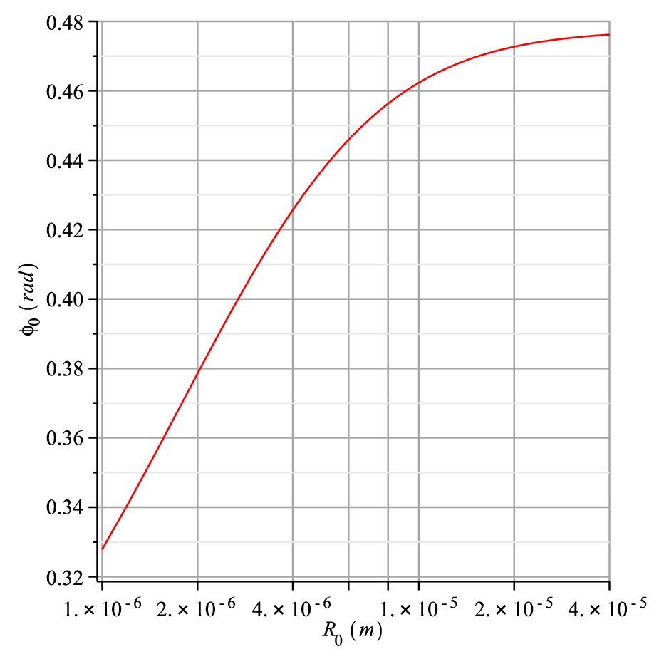
From Fig. 6, we observe a strong sensibility of $\phi_{0}$ in the range $R_{0}\in\left[1,\,6\right]\mu m$. Beyond that, specially in the range $R_{0}\in\left[10,\,40\right]\mu m$, we notice a weak modification on $\phi_{0}\in\left[0.46;\,0.48\right]\,rad.$ It is on the latter range that we can compare our algebraic results with experimental data.

In the published literature, we find the details on the obtaining the experimental data of optical birefringence pattern created by general nematic director fields in cylindrical capillaries [30, 45, 46, 47, 48, 49, 50] via optical polarizing microscopy and specifically by an escaped radial disclination [6, 15, 41, 51]. These birefringence patterns are produced for different orientations between the cylindrical axis and the polarization (analyzer) direction, represented by the angle $\alpha_{0}$ in Fig. 7.

Once our geometric approach for light propagation deals with scalar waves and it produces only one maximum of interference, we compare our analytic result with the experimental and numerically simulated data for liquid crystal E7 confined in capillary tubes of radius $R_{0}=14.25\,\mu m$ and $R_{0}=25.00\,\mu m$ [15]. The details of the experimental setup and of the numerical calculations can be found in [51]. For $R_{0}=14.25\,\mu m,$ we feed Eqs. $\left(\ref{sigma-general}\right)$, $\left(\ref{eq:b-expression}\right)$ and $\left(\ref{eq:angle-maximum-scattering}\right)$ with information found in [15], resulting in $\sigma=9.580$, $b=1.1759$ and our algebraic prevision of maximum interference at the angle $\phi_{0}\approx 26.93\text{\textdegree}$. Considering that the spatial scales of the experimental textures and numerically simulated ones shown in Figs. 8 and 9 refer to a screen positioned at the wall of the capillary tube of radius $R_{0}$, following the experimental arrangement shown in [51], we can infer the angle of each maximum in those interference patterns and localize, by red lines in those figures, our forecast angle of maximum of interference at $\phi_{0}=\pi\left(1-\frac{1}{b}\right)\approx 26.93\text{\textdegree}$ (the angular aperture from the center of the optical texture until the location of the forecast maximum of the differential scattering cross section). We observe that the calculated $\sigma=9.58$, where it were used the experimental data from [15], is different from the simulated one, $\sigma_{sim}=11$, needed to match the simulated texture with the experimental one. Once such discrepancy doesn’t occur for the capillary tube with $R_{0}=25\ \mu m$, as can be seen in the remaining of this section ($\sigma=15.2$ and $\sigma_{sim}=15$), we believe there was some mistype in [15] on the value of $\sigma_{sim}$ for $R_{0}=14.25\ \mu m$, that should be $\sigma_{sim}\approx 9.58$.

For wavelength $\lambda_{0}=435\,nm$ and $\alpha_{0}=45\text{\textdegree}$, one observes that our algebraically predicted angle $\phi_{0}$ is near to the outer end of the largest maximum of the experimental data (disregarding the central one) in Fig. 8a and it is near to the outer end of the correspondent computational predicted maximum in Fig. 8b. For wavelength $\lambda_{0}=589\,nm$ and $\alpha_{0}=45\text{\textdegree}$, the algebraically predicted angle $\phi_{0}$ is about at the middle point between two maxima of interference from the experimental data, as it can be seen in Fig. 8c, and it is near to outer end of the largest computational predicted maximum, as it can be seen in Fig. 8d. For $\alpha_{0}=0\text{\textdegree}$, independent of the used wavelengths, the algebraically predicted angle $\phi_{0}$ is far from any maximum of interference.

Before proceeding, a comment must be done about such results on the case of $\alpha_{0}=0\text{\textdegree}$. The lack of matching between our analytic prevision and the computational or experimental data can be explained as an effect of the polarizing of light by the liquid crystal at the surface of the tube. Using the data of the liquid crystal E7 weakly anchoring in a capillary tube of $R_{0}=14.25\,\mu m$, we obtain $\chi_{s}\approx 83\text{\textdegree\ }$, that is almost perpendicular to the analyzer filter, justifying the absence of light at our predicted angle using $\alpha_{0}=0\text{\textdegree}$. The same argument is valid for the next case, that uses a capillary tube of $R_{0}=25\ \mu m$. Beyond that, the difference between the experimental and simulated patterns for $\alpha_{0}=45\text{\textdegree}$ can be explained by the assumption made by the authors of [15, 51] in not considering the bend of light by the liquid crystal on the formation the interference pattern, as done in [17].

We implement another comparison using a capillary tube with $R_{0}=25\,\mu m$ with E7, as it can be seen in Fig. 9. Again, for $\alpha_{0}=0\text{\textdegree}$, there’s no matching between $\phi_{0}=\pi\left(1-\frac{1}{b}\right)\approx 27.19\text{\textdegree}$ ($\sigma=15.2$, $b=1.178$), and any of the maxima of light from experiment and simulation, independently of the used $\lambda_{0}$. For $\alpha_{0}=45\text{\textdegree}$ and $\lambda_{0}=435\,nm$, we see that the algebraically predicted angle $\phi_{0}$ is near to the inner final of the largest maximum of interference in Fig. 9a and is near to the outer final of the largest computational predicted maximum in Fig. 9b. For $\lambda_{0}=589\,nm$, the algebraically predicted angle $\phi_{0}$ it is near to the largest maximum of interference in Figs. 9c and 9d. The difference between Figs. 8 and 9 is a manifestation of the sensibility of the interference pattern on the radius $R_{0}$ of the capillary tube.

Finally the previous analysis allow one to define the approximate location of $\phi_{0}$ in the experimental pattern: near to the outer end of the largest maximum of interference pattern, using $\alpha_{0}=45\text{\textdegree}$. With that definition, we conclude that our single maximum of interfered light with angular position $\phi_{0}$ always occurs in the experimental results and computational simulations shown in Figs. 8 and 9, extracted from [15]. From $\phi_{0}$, one obtains the saddle-splay elastic constant $K_{24}$, as shown in the next subsection. Observe that this definition was deliberately chosen so that our algebraically calculated $K_{24}$ matches the value of the computationally obtained $K_{24}$ of [15], where the latter results are in agreement with their experimental measurements.

Starting with the one constant approximation, we can use the presented algebraic method for $\phi_{0}$ to determine $S_{0}$ and $K_{24}$ . For that, we need to substitute the equations $\left(\ref{eq:b-expression}\right)$, $\left(\ref{eq:chi-s-one}\right)$ and $\left(\ref{eq:sigma-one}\right)$ in $\left(\ref{eq:angle-maximum-scattering}\right)$ using the data of the studied liquid crystal, resulting in

Thus, the substitution of two different pairs of $R_{0}$ and $\phi_{0}$ (two experimental results of $\phi_{0}$ for two different values of $R_{0}$) in $\left(\ref{eq:extracting-k24-one-constant}\right)$ allows us to have a solvable system of two equations and two unknowns: $\frac{S_{0}}{K}$ and $\frac{K_{24}}{K}$. And if we have the value of $K$, (for example, through the approximation $K\approx\frac{K_{11}+K_{33}}{2}$ [15]), $S_{0}$ and $K_{24}$ become completely determined.

Out of the one constant approximation and to form our system of equations with unknowns $S_{0}$ and $K_{24}$ , we need additionally to know the values of the elastic constants $K_{11}$ and $K_{33}$ and to use the expressions $\left(\ref{eq:chi-s-general}\right)$ and $\left(\ref{sigma-general}\right)$. By this procedure, we would have an equivalent expression for $\left(\ref{eq:extracting-k24-one-constant}\right)$ and we expect a better precision on the value of $K_{24}$ (and eventually on $S_{0}$).

However, as we chose to study radii of the capillary tube in the range of weak sensibility on $\phi_{0}$, as shown in Fig. 6, there is a strong sensibility on the values of $K_{24}$ and $S_{0}$ due to the measured $\phi_{0}$ from the experimental data. A first way to bypass this problem is to use radii of capillary tubes smaller than $10\ \mu m$, which corresponds to the region of strong sensibility for $\phi_{0}\left(R_{0}\right)$. Another possibility consists of using more than two capillary tubes to attribute to $K_{24}$ and $S_{0}$ averaged values.

As a test of our approach, we use it to give the first reported estimation of $K_{24}$ for the lyotropic chromonic liquid crystal (LCLC) Sunset Yellow FCF (SSY) [52, 53, 54, 55]. From the light scattering data of wavelength $\lambda=650\ nm$ for 31.5% (wt/wt) SSY at 298.15 K forming a twisted and escaped radial disclination [54] (that has a director field close to the capillary walls similar to the one of the escaped radial disclination), for $0.99\ M$ SSY’s refractive indices at 303.15 K and wavelength $\lambda=633\ nm$ [55], our method gives $K_{24}=2.1\ pN$. Despite having used different temperatures, wavelengths and concentrations of SSY on this estimation, the calculated value of SSY’s $K_{24}$ still obeys Ericksen’s inequality $K_{22}+K_{24}\leq 2K_{11}$ [56] when using the experimental values of $K_{11}$ ($K_{11}=4.3\ pN$) and $K_{22}$ ($K_{22}=0.70\ pN$) found in [53]. We also report the first estimation of the the surface anchoring strength $S_{0}$ between SSY and parylene-N, material that was used in [54] to produce the homeotropic anchoring of the TER disclination: $S_{0}=5.5\cdot 10^{-10}\ J/m^{2}$.

References

- [1] D.-K. Yang and S.-T. Wu, Fundamentals of Liquid Crystal Devices, John Wiley, New Jersey, 2006.
- [2] R. Baetens, B. P. Jelle and A. Gustavsen, Solar Energy Materials and Solar Cells, 2010, 94, 87.
- [3] J. Doane, Liquid Crystals: Their Applications and Uses, World Scientific, New Jersey, 1990.
- [4] P. Oswald and P. Pieranski, Nematic and cholesteric liquid crystals: concepts and physical properties illustrated by experiments, CRC press, 2005.
- [5] D. S. Miller and N. L. Abbott, Soft Matter, 2013, 9, 374.
- [6] G. Crawford, D. W. Allender and J. Doane, Physical Review A, 1992, 45, 8693.
- [7] P. Boltenhagen, O. Lavrentovich and M. Kleman, J. Phys. II France, 1991, 1, 1233.
- [8] P. Boltenhagen, M. Kleman and O. D. Lavrentovich, J. Phys. II France, 1994, 4, 1439.
- [9] P. Boltenhagen, O. Lavrentovich and M. Kleman, Physical Review A, 1992, 46, R1743.
- [10] A. Sparavigna, O. D. Lavrentovich and A. Strigazzi, Phys. Rev. E, 1994, 49, 1344–1352.
- [11] E. Pairam, J. Vallamkondu, V. Koning, B. C. van Zuiden, P. W. Ellis, M. A. Bates, V. Vitelli and A. Fernandez-Nieves, PNAS, 2013, 110, 9295–9300.
- [12] P. Cladis and M. Kleman, J. Physique, 1972, 33, 591.
- [13] M. Kleman and O. D. Lavrentovich, Soft Matter Physics: an introduction, Springer-Verlag, New York, 2003.
- [14] P. A. Kossyrev and G. P. Crawford, Molecular Crystals and Liquid Crystals, 2000, 351, 379–385.
- [15] R. D. Polak, G. P. Crawford, B. C. Kostival, J. W. Doane and S. Zumer, Phys. Rev. E, 1994, 49, R978.
- [16] C. Sátiro and F. Moraes, Eur. Phys. J. E, 2006, 20, 173:1–6.
- [17] E. Pereira and F. Moraes, Liq. Crys., 2011, 38, 295–302.
- [18] E. R. Pereira and F. Moraes, Cent. Eur. J. Phys., 2011, 9, 1100–1105.
- [19] E. Pereira, S. Fumeron and F. Moraes, Physical Review E, 2013, 87, 022506.
- [20] S. Fumeron, B. Berche, F. Santos, E. Pereira and F. Moraes, Phys. Rev. A, 2015, 92, 063806.
- [21] S. Fumeron, E. Pereira and F. Moraes, Physica B, 2015, 476, 19–23.
- [22] S. Fumeron, E. Pereira and F. Moraes, Int. J. Therm. Sci., 2013, 67, 64–71.
- [23] S. Fumeron, E. Pereira and F. Moraes, Phys. Rev. E, 2014, 89, 020501.
- [24] D. Melo, I. Fernandes, F. Moraes, S. Fumeron and E. Pereira, Physics Letters A, 2016, 380, 3121 – 3127.
- [25] A. A. Joshi, J. K. Whitmer, O. Guzman, N. L. Abbott and J. J. de Pablo, Soft Matter, 2014, 10, 882–893.
- [26] R. R. A.J. Leadbetter and C. Colling, J. Phys. C1, 1975, 36, 37–43.
- [27] M. Kleman and L.Michel, Phys. Rev. Lett., 1978, 40, 1387–1390.
- [28] M. Kleman and G.Toulouse, J. Phys. Lettres, 1976, 37, 149–151.
- [29] G. Volovik and V. Mineev, Sov. Phys. JETP, 1977, 45, 1186–1196.
- [30] P. G. de Gennes and J. Prost, The Physics of Liquid Crystals, Claredon Press, Oxford, 2nd edn, 1992.
- [31] S. Burylov, Sov Phys JETP, 1997, 85, 873–886.
- [32] M. Born and E. Wolf, Principles of optics: electromagnetic theory of propagation, interference and diffraction of light, Cambridge university press, 1999.
- [33] W. Gordon, Annalen der Physik, 1923, 377, 421–456.
- [34] P. Alsing, American Journal of Physics, 1998, 66, 779–790.
- [35] M. Novello and J. M. Salim, Phys. Rev. D, 2001, 63, 083511.
- [36] U. Leonhardt and P. Piwnicki, Phys. Rev. Lett., 2000, 84, 822–825.
- [37] S. M. Carroll, Spacetime and geometry, Addison Wesley, San Francisco, 2003.
- [38] C. W. Misner, K. S. Thorne and J. A. Wheeler, Gravitation, W. H. Freeman and Company, San Francisco, 1973.
- [39] R. D’Inverno, Introducing Einstein’s Relativity, Oxford University Press, Oxford, 1998.
- [40] A. Vilenkin and E. Shellard, Cosmic strings and other topological defects, Cambridge University Press, Cambridge, 1994.
- [41] G. P. Crawford, J. A. Mitcheltree, E. P. Boyko, W. Fritz, S. Zumer and J. W. Doane, Appl. Phys. Lett., 1992, 60, 3226–3228.
- [42] D. W. Allender, G. Crawford and J. Doane, Physical review letters, 1991, 67, 1442.
- [43] C. Cohen-Tannnoudji, B. Diu and F. Laloe, Quantum Mechanics, Wiley-Interscience, New York, 1982, vol. 2.
- [44] G. B. Arfken, H. J. Weber and F. E. Harris, Mathematical methods for physicists: A comprehensive guide, Academic press, 7th edn, 2013.
- [45] R. B. Meyer, Philosophical Magazine, 1973, 27, 405.
- [46] C. Williams, P. Pieranski and P. E. Cladis, Phys. Rev. Lett., 1972, 29, 90.
- [47] C. E. Williams, P. E. Cladis and M. Kleman, Molecular Crystals and Liquid Crystals, 1973, 21, 355.
- [48] A. Saupe, Molecular Crystals and Liquid Crystals, 1973, 21, 211.
- [49] M. Kleman, Points, Lines and Walls in Liquid Crystals, Magnetic Systems and Ordered Media, Wiley, New York, 1988.
- [50] M. Kuzma and M. M. Labes, Molecular Crystals and Liquid Crystals, 1983, 100, 103.
- [51] A. Scharkowski, G. P. Crawford, S. Zumer and J. W. Doane, J. Appl. Phys., 1993, 73, 7280.
- [52] S.-W. Tam-Chang and L. Huang, Chemical Communications, 2008, 1957–1967.
- [53] S. Zhou, Y. A. Nastishin, M. Omelchenko, L. Tortora, V. Nazarenko, O. Boiko, T. Ostapenko, T. Hu, C. Almasan, S. Sprunt et al., Physical review letters, 2012, 109, 037801.
- [54] J. Jeong, L. Kang, Z. S. Davidson, P. J. Collings, T. C. Lubensky and A. Yodh, Proceedings of the National Academy of Sciences, 2015, 112, E1837–E1844.
- [55] V. R. Horowitz, L. A. Janowitz, A. L. Modic, P. A. Heiney and P. J. Collings, Physical Review E, 2005, 72, 041710.
- [56] J. Ericksen, Physics of Fluids (1958-1988), 1966, 9, 1205–1207.