USTC-ICTS-16-15
On Friedrichs Model with Two Continuum States
Abstract
The Friedrichs model with one discrete state coupled to more than one continuum is studied. The exact eigenstates for the full Hamiltonian can be solved explicitly. The discrete state is found to generate more than one virtual state pole or more than one pair of resonance poles in different Riemann sheets in different situations. The form factors could also generate new states on different sheets. All these states can appear in the generalized completeness relation.
I Introduction
Due to the intense experimental activities, more and more heavy quarkonium-like states were found these years in hadron spectroscopy as listed in the Particle Data Group Table [1]. However, many hadron states near or above the open-flavor thresholds can hardly be explained in the conventional “quenched” potential models, in which a meson state is regarded as the bound state of a quark and an anti-quark with a coulomb potential term at short distance and a linear confinement potential term at large distance, such as the Godfrey-Isgur (GI) model [2]. The discrepancies between the experiments and the potential model calculations seem to be made up by considering the couplings of the quark-antiquark bound states and the continuum hadronic states in different realizations, such as the coupled-channel model [3, 4, 5], and the screened potential model [6]. This mechanism also plays an important role when a discrete state is coupled strongly with more than one continuum states. Typically, the enigmatic and resonances in and scatterings [7, 8] can hardly be accommodated in the conventional quark model, because they are strongly coupled with the continuum states. In Ref. [9], most of the meson states below 2 GeV are found to be related to the resonance poles generated by a few bare states coupled with several thresholds, and some of the resonant states share the same origin of the bare state. In Ref. [10, 5], some of the charmed, charmed-strange, and charmonium-like states are discussed in the same spirit, where the inclusion of the hadron-loop effects causes the masses and widths of the states near or above the thresholds shifting from the GI’s prediction closer to the experimental data. With these coupling of the bare states and the continuum states, one would expect that the discrete bare states are no longer the eigenstate of the Hamiltonian and the resonance found in the experiments should be a linear superposition of the original discrete state and the continuum states. It would be desirable if one could describe the wave function of the resonance in terms of the discrete state and the continuum states.
The Friedrichs model [11, 12] is a kind of solvable model which couples a discrete state to a continuum state. The generalized eigenstates of the full interacting Hamiltonian, can be solved explicitly in terms of the original discrete state and the continuum states. The discrete state may become unstable and be described by Gamow states. These states can not be described by the vectors of the usual Hilbert space but by the ones in Rigged Hilbert Space (RHS)[13]. RHS is composed of a Gel’fand triplet , where is the usual Hilbert space of the normalizable states, is a nuclear space which is dense in , and is the space of the anti-linear continuous functionals on the nuclear space. Gamow states must be in the larger , since it is the generalized eigenstate of the full Hamiltonian with complex eigenvalues. The descriptions of the in-states and the out-states are using different Rigged Hilbert spaces, , where the subscript “” denotes the out-state space and “” denotes the in-state space. The triplet of state spaces can be mapped to the complex function spaces where , respectively, to form a representation. is the Schwarz space and is the so-called Hardy space in which the functions are analytic on and means restriction on . There are also two kinds of Gamow states, , denoting the decaying state and growing states which correspond to the lower and upper second sheet poles of the -matrix, respectively. For further detailed discussions on the mathematical foundation, the readers are referred to [14, 15].
In the original Friedrichs model where only one discrete and one continuum state are involved, the number of the discrete state poles generated from the original discrete state is doubled on the two-sheeted Riemann surface of the analytically continued -matrix. If the energy of the original discrete state is below the threshold, it will generate a bound state pole on the first sheet and a virtual state pole on the second sheet of the Riemann surface [16]. For the original discrete state with its mass higher than the threshold, it becomes a pair of resonance poles on the second sheet for small coupling. There can also be poles generated by the the form factor [17]. In our previous paper [16], we gave a general argument that for each simple pole of the form factor, there will be a second-sheet pole of the -matrix generated from this pole. The similar argument can also be applied to the exponential form factor and it can be demonstrated that there should be a virtual state pole generated from the minus infinity.
Some extensions of the original Friedrichs model to more than one system are made, most of which deals with more discrete states coupled with a continuum such as in Refs. [18, 19, 20, 21, 22]. It is also extended to include the fermion-boson interactions [23, 24]. In the present paper, we will extend the Friedrichs model to describe the process of coupling one discrete state with more than one continuum states with different thresholds, which is more relevant to the phenomenological studies of hadron spectroscopy, such as the hadron-loop models and the coupled-channel models. We mainly consider the scenario of including two continua, and then it is straightforward to generalize the result to the cases with more than two continua. The explicit solutions of the Friedrichs model with one discrete state coupled to two continua are presented, which is not found in the literature. Furthermore, in the two-continuum Friedrichs model, since the analytically continued -matrix is defined on a four-sheeted Riemann surface, the number of the discrete state poles will be doubled twice. For small couplings, we will discuss on which sheet the poles could be located in different conditions. These poles could be bound states on the first sheet or virtual states and resonances on the other sheets. All these states can be expressed as the superposition of the original discrete state and the continuum states. From the mathematical point of view, as in the single-continuum case, the singularity of the form factor can also generate states on different sheets.
In the original formulation of Friedrichs, only the continuum and the bound states could enter the completeness relation. However, Petrosky, Prigogine and Tasaki (PPT) [25] proposed a way to define the continuum in terms of a kind of complex distribution, in which the prescripted contour information of the energy are encoded in the continuum right eigenstates. In this formulation, the states corresponding to the unphysical sheet poles could also enter the completeness relation. We also generalize this kind of formulation to the multi-continuum cases, in which all the bound states, virtual states, and resonances are included in the completeness relation equally.
We organize the paper as follows: Section II gives the continuum solution to the Friedrichs model with one discrete state and two continua. Section III discusses the possible pole positions for small couplings. Section IV discusses the discrete states solutions in this model and the completeness relation. Section V generalizes the results to Friedrichs models with more than two continua. Section VI devotes to the conclusion and discussions.
II Solution to Friedrichs model with one discrete state and two continua
Suppose the full Hamiltonian is in which the free Hamiltonian has one discrete eigenstate and two kinds of continuum eigenstates, and , that is,
| (1) |
The continuum states are coupled to the discrete state with the coupling strength denoted by and respectively, and there is no direct interaction between the two continua. The interaction term of the Hamiltonian can be expressed as
| (2) | |||||
where and are the thresholds for the two continua in the energy representation with . Suppose the eigenstate of is expressed as
| (3) |
Then, a group of equations are obtained from the eigenequation ,
| (4) | |||||
| (5) | |||||
| (6) | |||||
To solve these equations, we distinguish three cases.
Case a) When , the solutions to Eqs. (5) and (6) are
| (7) | |||||
| (8) |
Inserting them into Eq.(4), we have the equation
| (9) |
where and . If this equation has solution on the real axis, the corresponding eigenvector will represent a bound state which is the renormalized state of the discrete unperturbed state . If this happens, since the two integrals are negative, must be less than , which means that the interaction pulls down the energy of the discrete state. A necessary condition for this to happen is
| (10) |
If it will guarantee that the system has a bound state. Moreover, the function can be analytically continued to a four-sheeted Riemann surface since it has two cuts. We will see that may also have zeroes on the second, third, and fourth sheets. In these cases, these zero points are complex generalized eigenvalues on different Riemann sheets and the corresponding generalized eigenstates can also be obtained. From Eq.(3), the eigenstate is recast into
| (11) |
These are generalized eigenstates with discrete eigenvalues which are zero points of the analytically continued . For bound states, the normalization can be chosen as such that . We will discuss more about these discrete states later.
Case b) When , since Eq.(6) only exists in , only can have function contribution
| (12) | |||||
| (13) |
We have inserted the in the denominator to avoid the singularity at . Inserting them into (4), we then have
| (14) |
If we define
| (15) |
can be expressed as
| (16) |
With the choice of the normalization such that , the eigenstate for eigenvalue can then be obtained
| (17) |
In Eqs. (15) and (17) the ’s in the last integrals has no effect for , but we keep them in order to extend these equations to case below.
Case c) Let us now look at . There are two degenerate states for the free Hamiltonian. We would expect that there are also two degenerate eigenstates of the full Hamiltonian for these eigenvalues. From Eq. (5) and Eq. (6), Eq. (12) is not changed and Eq. (13) becomes
| (18) |
It is obvious that the solution of Case b) is also the solution for this case with . If the couplings are turned off, this solution goes back to . There must be another solution which becomes as . We start with ansatz (18) and set in (12), and then have
| (19) |
Similar to Eq. (17), after choosing the suitable normalization such that , we then obtain the other solution for eigenvalue ,
| (20) |
It can be proved that .
In general, for eigenvalue , the eigenstate solution should be a superposition of Eqs. (17) and (20). is the in-state and is the out-state. The function defined in (9) and in (15) can be analytically continued to one function defined on a four-sheeted Riemann surface, which we also denote as , with and being the boundary functions on the upper rim and lower rim of the cut on the first sheet. From case a), the poles of on the different Riemann sheets are the discrete eigenvalues and the corresponding states may represent the bound states, virtual states, and resonant states for the full Hamiltonian. Before studying these solutions, we will first study the pole behaviors for for small couplings in the next section.
III Analysis of the pole positions for weak couplings
As in the discussion of the simplest Friedrichs model [16], we choose form factors and with , to illustrate the general behaviors of the poles for small couplings. The two thresholds for are at and with . The analytically continued -matrix or function will have four Riemann sheets and we define the second sheet to be the one analytically continued from the cut between and on the first sheet, the third sheet to be continued from the cut above on the first sheet, and the fourth sheet to be continued from the cut above on the second sheet or from the cut between and on the third sheet. See Fig. 1 for illustrations.


In the simplest Friedrichs model with one continuum, it was shown that the poles of the form factor always introduce poles of near these singularities on the unphysical sheet [16]. Now there are two form factors, we will see that the singularities of them will also generate different poles on different Riemann sheets. From the definition of , Eq. (15), there are two integrals in the definition. In each integral, the form factor provides a pole to the integrand, which introduces a pinch singularity of at on both the second sheet and the third sheet for the first integral, and a pinch singularity at on both the third sheet and fourth sheet for the second integral. In fact, the function on each sheet can be represented as,
| (21) | ||||
| (22) | ||||
| (23) |
in which and are analytically continued from the real axis to the first Riemann sheet, and , , , label the first, second, third, and fourth sheets, respectively. The analytically continued should satisfy the Schwartz reflection relation , which is the so-called real-analytic function. Thus, the analytically continued , which are proportional to the imaginary parts of the integral, should satisfy on each sheet, which will be called anti-real-analytic function here. From above equations, the poles in and/or in each equation are just the pinch singularities for the analytically continued on the corresponding sheet.
Similar to the argument in the single-continuum case in Ref. [16], near the pole of , i.e. near on the second sheet and the third sheet in our example, the form factor will generate a zero point of on each of these two sheets. The argument goes as follows: near , on the second sheet and the third sheet takes the form of
| (24) |
where and are real functions on the real axis below the lowest threshold and regular at . At limit both and are the solutions to the right equation and are first-order zero points, though, at exact , is not the solution for the left equation. When goes away from zero, on the real axis will still be real below the threshold and be deformed smoothly. So, the solutions originating from will not disappear and just moves away on the real axis. Similar argument can be applied to . Thus, each pole of the integral generated by the form factor on each sheet will introduce a virtual state near it for small couplings. To sum up, for small enough and , there are virtual state poles generated around on the second and the third sheets, and around on the third and fourth sheets. The typical shape of the on different sheet below the first threshold are shown in Fig. 2. This argument applies to the general form factors with simple poles below the lowest threshold or with a pair of simple poles on the complex plane. If the form factors has multi-poles, for example, a second-order pole below the threshold on the real axis, the poles on the unphysical sheet may also move away onto the complex plane becoming resonance poles by the similar argument. If in some accidental cases, , since on the third sheet the two poles of the integrals are combined together, Eq. (24) becomes
| (25) |
Thus, on the third sheet, there would be only one simple pole generated by the two form factors. See Fig. 3(a) for an illustration.


We then look at the poles generated from the original discrete state. For , at , has the solution . Similar to the virtual state poles generated by the form factors, as are turned on, since near both integrals in are real on each sheet, is only continuously corrected by a small real part on the negative axis on each sheet, and hence the original solution at is copied on each sheet and moves away from on the real axis. So, originating from the discrete state at , there are one bound state on the first sheet and one virtual state pole on each unphysical sheet for small enough couplings. See Fig. 2 for an illustration. Since these poles are below the lowest threshold, only the bound state pole and the virtual state pole on the second sheet are close to the physical region so that they may have observable effects in experiments.


Concerning the virtual state poles from the form factors, there could be another accidental case where and . In this case, Eq. (24) can also be used with . For the example form factors, it can be proved that . If we turn on first and then turn on slowly, the pole of generated by and the pole generated near on each sheet where both appear would go into the complex plane and become a pair of resonance poles symmetric with respect to the real axis. See Fig. 3 for an illustration. If for some form factors, , the two poles will separate on the real axis. If we turn on first and then turn on , the two virtual state poles would separate first on the real axis for small enough couplings. The other accidental case where and can also be discussed similarly. The most accidental case is that where Eq.(25) can also be used with . In this case, the two poles of the integrals from the form factors would combine as discussed previously and on each unphysical sheet the two solutions generated by and the form factors would go into the complex plane and become resonance poles if the right hand side of Eq.(25) is negative as for our example form factors (Fig. 4), otherwise they will separate on the real axis.


For , when , and small enough, we reduce to the single-continuum case, in which there is a bound state on the first sheet and a virtual state on the second sheet generated from [16]. Then when is turned on, the first sheet is duplicated to be the first and the second sheet and the old second sheet is duplicated to be the third and the fourth sheet. The old bound state on the first sheet will obtain finite decay width and move onto the second sheet becoming a pair of resonance poles as shown in Fig. 5. This can be understood as follows. The analytically continued on the first sheet and the second sheet can be represented as
| (26) | ||||
| (27) |
For on the upper plane (we take and of the same order here), the first integral term contributes a positive imaginary part to , . The second integral also gives a positive imaginary part . Since the integral in the only has a positive imaginary part near on the upper half plane, there could not be a solution on the first sheet as the couplings are turned on. However, the last term in of the second sheet provides a negative imaginary part around . So, the solution to must move from the original first sheet to the second sheet and for real analyticity, the solutions should be symmetric with respect of the real axis. This is consistent with the causality. This argument is independent of the specific form factors chosen.


Similarly, the original virtual state on the old second sheet when only is turned on will move to the third sheet for the chosen example form factors, which can be seen as follows. on the third and fourth sheet can be represented as
| (28) | ||||
| (29) |
For with imaginary part on the upper plane, will have imaginary part which can not cancel the imaginary part of . Only the on the third sheet can cancel the imaginary part and there can be solutions in the third sheet complex plane as is turned on. Thus, the pole will move onto the third sheet. This argument also applies for general form factors. This is because gives the imaginary part of the second integral, and should be real-analytic and has a cut starting from . Below the branch point of the cut, it is continuous and should be real by real-analyticity. So, for , the imaginary part of is always of . Thus, the above argument applies and in general the poles will move to the third sheet.
Alternatively, we could turn off , and turn on first, and the discrete state will move to the second sheet to be a pair of resonance poles in the reduced single-continuum case. Then when we turn on slowly, the first sheet will be doubled to become the first and the fourth sheet and the second sheet will be duplicated to be the second sheet and the third sheet with the resonance poles also copied to both sheets and corrected by . This argument also applies for other general form factors and the result is consistent with the one in the previous paragraph. Turning on which coupling first may give different trajectories though their final positions can be the same.
The last case is when the discrete state is above the second threshold . Similar to the above analysis, if , and is turned on, then the discrete state will move to the second sheet becoming a pair of resonance poles and will not appear on the first sheet. When we turn on , the old first sheet will be duplicated to be the first sheet and the fourth sheet. So, on these two sheets there is no pole originating from the discrete state for small enough . The second sheet will be duplicated to be the second sheet and the third sheet, both carrying the resonance poles originated from the discrete state. So, similar to above case, the discrete pole will generate one pair of resonance poles on the second sheet and another pair on the third sheet.
However, if we first turn on , the discrete state will become the resonance state on the second sheet. When we then turn on slowly, the old first sheet becomes the first and the second sheets, and thus there are no poles moving onto these two sheets for small enough . The old second sheet becomes the third and the fourth sheet carrying the resonance pole. Therefore, in this case the discrete state becomes the resonance states on the third and the fourth sheets as shown in Fig. 6. As becomes larger to some extent, the fourth sheet pole may run across the second cut moving to the second sheet as if we turn on first and then turn on . See Fig. 7 for an illustration.


From the above discussions, we have observed that when one bare discrete state is coupled to more than one continuum states with different thresholds, there could be more than one pair of resonance poles generated from this discrete state. We have two thresholds here and the number of the Riemann sheets is four which doubles the ones when there is only one continuum. The poles on the Riemann sheets will also be duplicated and thus the number of the poles will also be doubled.
IV Discrete states and the completeness relation
We have seen that there could also be poles on the second, third and fourth sheets. One can prove that the bound state if exists, and these two continuum states form a set of complete basis,
| (30) |
However the other discrete states on unphysical sheets do not enter the completeness relation.
In the simplest Friedrichs model, in Ref. [25], in order to solve the large Poincaré problem and based on two physical conditions: the decay of unstable state in the future and the emission of out-going wave, PPT take the continuum states as a complex functional and choose a kind of the integral contour for in the continuum states, and then all the discrete states enter the completeness equation equally. In their discussion, the original discrete state is defined to be a little above the real axis, and the integral path on the real axis is below the discrete state. After the coupling is turned on, the discrete state goes below the real axis to the second sheet complex plane, and the integral contour should also be deformed to the lower half plane, below the pole of the discrete state. In Ref. [16], we also found that all the second sheet poles could merge and separate, and these poles should not be treated differently, whether they are generated from the discrete state or from the form factor. The integral path for the continuum state should be deformed to the second sheet around all the poles on the lower half of the second sheet like the one in Fig. 8. After this modification to the continuum state, all the discrete states including the ones on the second sheet enter the completeness relation. Here, we can generalize this kind of definition to the two-continuum case.

In this spirit, we need to choose the integral contour for in the in for coupled channel cases. If we turn off one of the couplings, we come back to the single-continuum case and the contour should be the same as in the single-continuum case. So, the integral contour should go from the first sheet to each sheet around all poles and back to the first sheet along the positive real axis to the infinity as shown in Fig. 9. To be specific, if there are (, ) second (third , fourth) sheet poles, including the poles generated from the form factors, similar to [25], the in the continuum right eigenstate in Eqs. (17) and (20) should be modified to
| (31) |
This equation just means that we put the integral path information in the definition of through , where means the integral path of is continued as shown in Fig. 9, and means just the opposite.
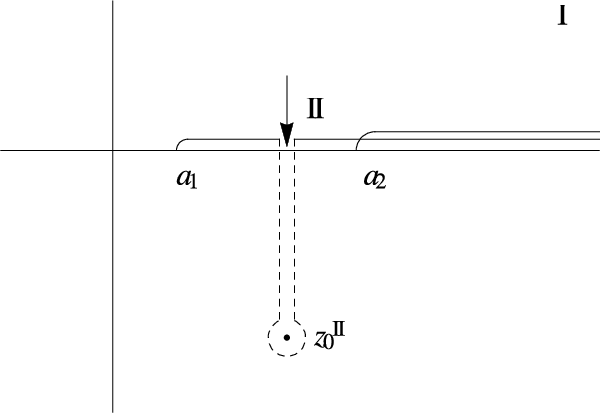


In the left eigenstates the definition of the integral path on the real axis is not modified, since there is no pole for continued downward from the lower edge of the cut on the first sheet to the lower half plane. As in [25], this kind of choice of the contour is consistent with two physical conditions, i.e., the decay of unstable state in the future and the emission of out-going wave. So the right and left continuum eigenstates can be expressed as
| (32) | |||
| (33) |
and orthogonal relations are not modified, .
We have shown that there will be more than one Gamow states corresponding to one original discrete state and could also be other states generated from the form factors. Since the poles can lie on the unphysical sheets, the integral in the expression of the states need to be analytically continued to different sheets and the integral path should be deformed accordingly, that is,
| (34) | ||||
| (35) | ||||
| (36) | ||||
| (37) |
which are the generalized eigenstates of with eigenvalue on the lower half plane of the -th sheet with , including the real axis below the lowest thresholds. Since the two integrals defines the two cuts independently, the integral path can be defines separately for each integral. The means the continuation from upper half of the Riemann sheet to the pole positions on the other Riemann sheets, through the first cut in the first integral or through the second cut in the second integral, which requires the integral paths to be deformed accordingly. For example, the third sheet is reached by going through both cuts above the second threshold; therefore both integral paths are deformed. To simplify notation, we encode the contour information into the pole position, denoted by , for , in which the subscript “” means continuation from upper to lower sheets and “” means the opposite, and from one can determine whether the continuation across the cut is needed or not. One can then unify the states in the four sheets to be
| (38) |
For example, if , only the first integral is continued downward and the second integral is not. It is easy to check directly that . The left eigenstates with the same eigenvalue as the corresponding right eigenstates can also be solved,
| (39) |
The normalization constants are chosen to be such that for . These states on different sheets can be proved to be orthogonal to each other, for .
As we stated, in the case with one continuum, after including the integral path into the continuum states, the resonance poles and the virtual state poles also enter the completeness relations [25, 16]. In two-continuum case, one discrete state is split onto different Riemann sheets to be different resonant states or virtual states. There are also other virtual states or resonances generated by the form factors. It is expected that all these discrete states enter into the completeness relation using the continuum states defined above. This can be proved as expected
| (40) |
where , for poles on the -th sheet. We consider only simple poles here. In [16], the poles are found to merge to be higher order poles and separate for larger couplings. Similar things could also happen here, and the same discussion in the one-continuum case also applies which will not be repeated here.
V More than two continuum states
We have discussed the solutions for Friedrichs model with two continuum states. It is straightforward to extend the solution to the model with more than two continua. Suppose that there are continuum states coupled to a discrete state without the direct couplings among the continua, described by the Hamiltonian
| (41) | |||||
The continuum state solutions for the full Hamiltonian can be obtained similar to Eqs. (17) and (20):
| (42) |
where
| (43) |
Whenever there is an additional continuum included, on each Riemann sheet there is a new cut and analytically continuation will double the Riemann sheets. Thus there are Riemann sheets. The discrete states also correspond to the zero points of the analytically continued and will be carried to the duplicated Riemann sheets and be renormalized separately. Thus, the number of the poles generated by the original discrete states will also be . The poles introduced by the form factors will also be copied on the duplicated Riemann sheets when the other continua channels are included, and hence the number for each such poles will be except some accidental cases as discussed in Sect. III. All the previous discussions can be extended to here without any difficulty. We will not repeat it here. Although there are so many poles on the unphysical sheets, only those near the physical region may have observable effects in the experiments.
VI Conclusion and discussions
In this paper we have first discussed the solution for the Friedrichs model with one discrete state coupled to two continuum states with different thresholds. The generalized eigenvalues for the full Hamiltonian include the continuum spectra and all the zero points for the on the four-sheeted Riemann surface. The generalized eigenstates for the continuum spectra are expressed in Eq. (17) and Eq. (20) which reduce to the original two continuum states when the couplings are switched off as expected. The original discrete state will generate poles on the four-sheeted Riemann surface of the analytically continued or -matrix. When the original discrete state is below the lowest threshold, it will become a bound state pole on the first sheet and three virtual state poles on the other three unphysical sheets for small couplings. When it is above the lowest threshold, it will move to the other unphysical sheets becoming two pairs of resonance poles on different sheets. There are also poles on different sheets generated by the form factors. From a mathematical point of view, for each simple pole of the form factor, there will be poles of generated on the unphysical sheets for small couplings except for some accidental cases. All these states can be expressed as the linear combinations of the original discrete states and continuum states explicitly. By generalizing the definitions of the continuum states of [25], these discrete states can also enter the completeness relation equally. All these discussions can then be generalized to Friedrichs model with more than two continuum states. For an -continuum model, the discrete state will generate poles while the number of the poles generated from the form factor will be . The bare discrete state may be viewed as the bound state at the more fundamental level such as the bound state of the quarks, which may be called “normal states”, whereas the states generated from the form factors can be viewed as bound states of the composite level such as the hadrons, which may represent the so called “molecular states”. So, we then have a theoretical criterion to distinguish the molecular states from the normal states, that is, the number of poles generated from the molecular state should be one half of the one for the normal state. This is consistent with the pole counting rule proposed by Morgan [26].
The poles on the different sheets with the same origins was noticed a long time ago by by Eden and Taylor when studying the property of the -Matrix, and these poles are called shadow poles[27]. However some of the shadow poles are too far away from the physical region and may not have observable effects in the experiments. Nevertheless, there could be cases that shadow poles may take effects in the experiments. In the last two cases in the analysis in Sect. III, when is near the second threshold, the resonances generated on the second sheet and third sheet could be close to the physical region and , respectively, and may both have observable effects in experiments. In fact, some shadow poles may have already been seen in the experiments. In recent years, we have seen more and more Quarkonium-like state and exotic state in the experiments, for example, , . In fact, in [28], a second sheet pole and a third sheet pole are found to be responsible for the and line shapes, and both poles originate from a common bound state. In [9] the low energy channel, a dozen of resonances are found to originate from only four bare states.
We expect that this discussion would be useful in studying the hadron spectrum, especially on the newly observed exotic states. In fact, the preliminary attempt has been made recently on the P-wave excited charmonium states and yielded good results [29]. Although our study was motivated by the phenomenology aspects in hadron interaction, the theory on resonances phenomenon can have much broader applications. Actually, the resonance phenomena are observed in different areas of modern physics, and there are also some variants of the Friedrichs model in various contexts. The Lee model [30] is a field theory realization of the Friedrichs model and there are other second quantized version of the Friedrichs model like in Refs. [31, 32]. In condense matter physics, the Fano-Anderson [33, 34] model is also similar to the Friedrichs model with a bounded continuum spectrum. Friedrichs-Fano-Anderson model is also used in atomic physics, quantum electrodynamics and statistical physics, such as in the study of the bound state in the continuum phenomena [35, 36, 37]. The results and the methods in our paper are rather general and may be helpful in understanding the diverse phenomena in these areas.
Acknowledgements.
Z.X. is supported by China National Natural Science Foundation under contract No. 11105138, 11575177 and 11235010.References
- [1] K. A. Olive et al. (Particle Data Group), Chin. Phys. C 38, 090001 (2014).
- [2] S. Godfrey and N. Isgur, Phys. Rev. D 32, 189 (1985).
- [3] M. R. Pennington and D. J. Wilson, Phys. Rev. D76, 077502 (2007), arXiv:0704.3384 [hep-ph] .
- [4] S. Coito, G. Rupp, and E. van Beveren, Eur. Phys. J. C73, 2351 (2013), arXiv:1212.0648 [hep-ph] .
- [5] Z.-Y. Zhou and Z. Xiao, Eur. Phys. J. A 50, 165 (2014), arXiv:1309.1949 [hep-ph] .
- [6] B.-Q. Li and K.-T. Chao, Phys. Rev. D79, 094004 (2009), arXiv:0903.5506 [hep-ph] .
- [7] Z. Xiao and H. Q. Zheng, Nucl. Phys. A695, 273 (2001), arXiv:hep-ph/0011260 [hep-ph] .
- [8] H. Q. Zheng, Z. Y. Zhou, G. Y. Qin, Z. Xiao, J. J. Wang, and N. Wu, Nucl. Phys. A733, 235 (2004), arXiv:hep-ph/0310293 [hep-ph] .
- [9] Z.-Y. Zhou and Z. Xiao, Phys. Rev. D 83, 014010 (2011a), arXiv:1007.2072 [hep-ph] .
- [10] Z.-Y. Zhou and Z. Xiao, Phys. Rev. D 84, 034023 (2011b), arXiv:1105.6025 [hep-ph] .
- [11] K. O. Friedrichs, Commun. Pure Appl. Math. 1, 361 (1948).
- [12] L. Horwitz and J. Marchand, Rocky Mountain J. Math. 1, 225 (1971).
- [13] I. E. Antoniou and I. Prigogine, Physica A: Statistical Mechanics and its Applications 192, 443 (1993).
- [14] A. Bohm and M. Gadella, Dirac Kets, Gamow Vectors and Gel’fand Triplets, edited by A. Bohm and J. D. Dollard, Lecture Notes in Physics, Vol. 348 (Springer Berlin Heidelberg, 1989).
- [15] O. Civitarese and M. Gadella, Phys. Rep. 396, 41 (2004).
- [16] Z. Xiao and Z.-Y. Zhou, Phys. Rev. D94, 076006 (2016), arXiv:1608.00468 [hep-ph] .
- [17] A. K. Likhoded and G. P. Pronko, Int. J. Theor. Phys. 36, 2335 (1997).
- [18] G. Stey and R. Gibberd, Physica 60, 1 (1972).
- [19] T. K. Bailey and W. C. Schieve, Il Nuovo Cimento A (1965-1970) 47, 231 (1978).
- [20] G. Ordonez and S. Kim, Phys. Rev. A 70, 032702 (2004).
- [21] I. Antoniou, E. Karpov, G. Pronko, and E. Yarevsky, International Journal of Theoretical Physics 42, 2403 (2003a).
- [22] M. Gadella and G. Pronko, Fortsch. Phys. 59, 795 (2011), arXiv:1106.5782 [math-ph] .
- [23] O. Civitarese and M. Gadella, Int. J. Mod. Phys. E15, 1273 (2006), arXiv:nucl-th/0703090 [nucl-th] .
- [24] O. Civitarese, M. Gadella, and G. P. Pronko, Int. J. Mod. Phys. E16, 169 (2007), arXiv:nucl-th/0703091 [nucl-th] .
- [25] T. Petrosky, I. Prigogine, and S. Tasaki, Physica 173A, 175 (1991).
- [26] D. Morgan, Nucl. Phys. A543, 632 (1992).
- [27] R. J. Eden and J. R. Taylor, Phys. Rev. 133, B1575 (1964).
- [28] Z.-Y. Zhou and Z. Xiao, Phys. Rev. D92, 094024 (2015), arXiv:1505.05761 [hep-ph] .
- [29] Z.-Y. Zhou and Z. Xiao, (2017), arXiv:1704.04438 [hep-ph] .
- [30] T. D. Lee, Phys. Rev. 95, 1329 (1954).
- [31] I. E. Antoniou, M. Gadella, J. Mateo, and G. P. Pronko, J. Phys. A36, 12109 (2003b).
- [32] E. Karpov, I. Prigogine, T. Petrosky, and G. Pronko, Journal of Mathematical Physics 41, 118 (2000), http://dx.doi.org/10.1063/1.533125 .
- [33] U. Fano, Phys. Rev. 124, 1866 (1961).
- [34] P. W. Anderson, Phys. Rev. 124, 41 (1961).
- [35] G. Duerinckx, Journal of Physics A: Mathematical and General 16, L289 (1983).
- [36] M. Miyamoto, Phys. Rev. A 72, 063405 (2005).
- [37] Longhi, S., Eur. Phys. J. B 57, 45 (2007).