Velocity segregation effects in galaxy clusters at
Abstract
Aims. Our study is meant to extend our knowledge of the galaxy color and luminosity segregation in velocity space (VCS and VLS, resp.), to clusters at intermediate and high redshift.
Methods. Our sample is a collection of 41 clusters in the redshift range, for a total of 4172 galaxies, 1674 member galaxies within 2 with photometric or spectroscopic information, as taken from the literature. We pay attention to perform homogeneous procedures to select cluster members, compute global cluster properties, in particular the LOS velocity dispersion , and separate blue from red galaxies.
Results. We find evidence of VCS in clusters out to (at the 97%-99.99% c.l., depending on the test), in the sense that the blue galaxy population has a 10-20% larger than the red galaxy population. Poor or no VCS is found in the High- sample at . For the first time, we detect VLS in non-local clusters and confirm that VLS only affects the very luminous galaxies, with brighter galaxies having lower velocities. The threshold magnitude of VLS is , where is the magnitude of the third brightest cluster galaxy, and current data suggest that the threshold value moves to fainter magnitudes at higher redshift. We also detect (marginal) evidence of VLS for blue galaxies.
Conclusions. We conclude that the segregation effects, when their study is extended to distant clusters, can be important tracers of the galaxy evolution and cluster assembly and discuss the poor/no evidence of VCS at high redshift.
Key Words.
galaxies: clusters: general – galaxies: kinematics and dynamics – galaxies: evolution – cosmology: observations1 Introduction
It is well established that the properties of cluster galaxies differ from those of field galaxies and that clusters are characterized by radial gradients. Galaxies in denser, central regions are usually of earlier morphological type, redder color, and lower star formation rate. This is the well-known phenomenon of the spatial segregation of spiral/elliptical galaxies and of blue/red galaxies in local and distant clusters (e.g., Melnick & Sargent 1977; Dressler 1980; Whitmore et al. 1993; Abraham et al. 1996; Dressler et al. 1999; Gerken et al. 2004). More recently, this effect is only questioned at very high redshift where some authors detect an inversion of the star formation rate vs. galaxy density (Tran et al. 2010; Santos et al. 2015, but see Ziparo et al. 2014). The spatial segregation is a basic observable in the framework of galaxy evolution and, in particular, of the connection between galaxy evolution and cluster environment.
A related phenomenon is the segregation of galaxies of different color/type in velocity space (hereafter VCS). Unfortunately, requiring a lot of observational effort to measure galaxy redshifts, this effect is far less known than the spatial segregation. Since the pioneering works of Tammann (1972) and Moss & Dickens (1977), several studies have reported significant differences in the velocity distributions of different galaxy populations. The velocity dispersion of the population of blue, star-forming galaxies is found to be larger than that of the population of red, passive galaxies (e.g., Sodré et al. 1989; Biviano et al. 1992; Scodeggio et al. 1995; Biviano et al. 1996; Colless & Dunn 1996; Mohr et al. 1996; Biviano et al. 1997; Adami et al. 1998; Dressler et al. 1999; Goto 2005).
Moss & Dickens (1977) suggested that VCS is an evidence of an infalling population of field galaxies into the clusters. Large data samples, obtained stacking galaxies of several clusters, have allowed to trace the velocity dispersion profiles (VDPs) and obtain new insights on the issue. Biviano et al. (1997) analyzed the ESO Nearby Abell Cluster Survey (ENACS – 107 clusters, see Katgert et al. 1996) and inferred that the kinematical segregation of the emission line galaxies (ELGs) with respect to the passive galaxy population reflects the time of infall rather than the virialized condition. In fact, they found that the VDP of ELGs is consistent with the fact that ELGs are on more radial orbits than passive galaxies. Carlberg et al. (1997) analyzed the Canadian Network for Observational Cosmology cluster sample (CNOC – 16 clusters at medium redshift , see Yee et al. 1996), finding that the blue galaxy population is characterized by a larger value of the global velocity dispersion than the red galaxy population and a different VDP. The difference in the VDP is an expected consequence of the fact that both populations trace the same cluster potential with different spatial density profiles. Biviano & Katgert (2004) have shown that early and late spectroscopic type galaxies of ENACS clusters are in equilibrium in the cluster potential and that late-type galaxies have more radially-elongated orbits. Some interesting papers have started to analyze cluster numerical simulations in the attempt to trace galaxies during their infall into clusters and relate galaxy properties to their position in the projected phase space or to the kinematical properties of the galaxy population, that is velocity distribution and velocity dispersion (e.g., Mahajan et al. 2011; Hernández-Fernández et al. 2014; Haines et al. 2015). In this context, VCS is therefore an important observational feature related to galaxy evolution during cluster assembly.
The presence of VCS is questioned in a few past and recent studies. Analyzing a sample of six clusters, Zabludoff & Franx (1993) found that the early- and late-type galaxies have no different velocity dispersions. The analysis of the Cluster and Infall Region Nearby Survey (CAIRNS – 8 clusters at , see Rines et al. 2003) have shown that the kinematics of star-forming galaxies in the infall region closely matches that of absorption-dominated galaxies (Rines et al. 2005). Hwang & Lee (2008) investigated the orbital difference between early-type and late-type galaxies in ten clusters using data extracted from SDSS and 2dFGRS data, in four of these they have not found any difference. Rines et al. (2013) analyzed the Hectospec Cluster Survey (HeCS – 58 clusters with ) obtaining that the determination of velocity dispersion and dynamical mass is insensitive to the inclusion of bluer members and that the velocity dispersion of the ensemble cluster of all galaxies is only 0.8% larger than that of the red-sequence galaxies.
The above-mentioned discrepancies can be probably understood taking into account that the analysis of VCS implies several difficulties and possible sources of confusion. The member selection is particularly critical since the effect of including typically blue, field galaxies can bias the velocity dispersion of the blue population towards higher values. Another difficulty is that the amount of VCS, detected so far, is quantitatively small, accounting for -20% (30% at most) of the value of the velocity dispersion. For a small velocity segregation, there is a strong spatial segregation and a decreasing trend of the VDP, in particular in the case of star-forming galaxies (Biviano & Katgert 2004). The last two effects combine in such way to hide the VCS effect when computing global values of the velocity dispersion, in spite of the positive detection in the VDP (e.g., Girardi et al. 2015). Indeed, most of the existing positive detections of VCS have been derived analyzing the VDPs of ensemble clusters obtained stacking together galaxies of many clusters. The price to be paid for the large gain in statistics when using ensemble clusters is that one averages away possible individual behaviors, that might explain the discrepancies above reported. Recent and ongoing cluster catalogs, based on hundreds of member galaxies per cluster (e.g., Owers et al. 2011), will allow us to study the VDP and VCS of individual clusters. MACS J1206.2-0847 is the first cluster of the CLASH-VLT survey (Rosati et al. 2014) where VCS has been analyzed (Girardi et al. 2015).
Moreover, to date, little is known about the velocity segregation in relation to cluster properties. For instance, the relation between VCS and cluster dynamical status has been explored in very few studies (Ribeiro et al. 2010; Ribeiro et al. 2013). The member selection might be particularly critical in very active clusters, and the scenario is made more complex by the fact that cluster mergers might also enhance star formation in galaxies (e.g., Caldwell & Rose 1997; Ferrari et al. 2005; Owen et al. 2005). The dependence of VCS with redshift is poorly investigated, too. The pioneering study of Biviano & Poggianti (2009), based on 18 clusters of the ESO Distant Cluster Survey (EDisCS – -0.8, see White et al. 2005), indicates that VCS is not as pronounced as in local ENACS clusters. Crawford et al. (2014) analyzed five distant clusters () finding that red sequence, blue cloud, and green valley galaxies have similar velocity distributions. To probe of VCS in distant clusters is on interest also in view of the spectroscopic survey to be provided by the ESA Euclid mission (Laureijs et al. 2011). Euclid will provide spectroscopic data for distant clusters at , but only for galaxies with H lines (Sartoris et al. 2016 and refs. therein). This raises the question as to how velocity dispersions measured using star forming galaxies compare with those usually measured with red galaxies. Understanding possible biases in the measurements of velocity dispersions using different galaxy populations has implication for cosmological applications of the distribution function of velocity dispersions (e.g., Borgani et al. 1997).
This paper is devoted to the study of VCS in distant clusters () and is based on the data of 41 clusters collected in the literature. To obtain further insights into the physical processes involved in the velocity segregation, we also analyzed the possible presence of luminosity segregation in velocity space (VLS) which is reported in the literature as a minor effect with respect to VCS (Chincarini & Rood 1977; Biviano et al. 1992 and refs. therein). In particular, Biviano et al. (1992) have found that only the most luminous galaxies are segregated in velocity, with brighter galaxies having lower velocities. This result has been confirmed in more recent papers (Adami et al. 1998; Goto 2005; Ribeiro et al. 2013) and in poor group environments (Girardi et al. 2003; Ribeiro et al. 2010). The observed phenomenology has been explained by physical processes that transfers kinetic energy from more massive galaxies to less massive ones. In particular, the dynamical friction (Sarazin 1986) is the most probable mechanism (Biviano et al. 1992; Mahajan et al. 2011).
The paper is organized as follows. We present our cluster catalog in Sect. 2. Sections 3 and 4 are devoted to the presentation of member selection, main cluster properties, and separation between red and blue galaxy populations. Section 5 concentrates on the analysis of the VCS and VLS effects, discussed in the following Sect. 6. We give our summary and conclusions in Sect. 7.
Unless otherwise stated, we give errors at the 68% confidence level (hereafter c.l.). Throughout this paper, we use km s-1 Mpc-1 in a flat cosmology with and .
2 Data sample
We collected data for clusters with redshift and sampled by at least galaxies with measured in the cluster field. In order to separate late-type/blue/star-forming galaxies from early-type/red/passive galaxies, we also required color or spectral information. In most cases we used the color information and, in the following, we refer to the two above classes of galaxies as blue and red galaxies. In the data collection we also made use of NED 11 1 The NASA/IPAC Extragalactic Database (NED) is operated by the Jet Propulsion Laboratory, California Institute of Technology, under contract with the National Aeronautics and Space Administration. looking for cluster data until 2015 June 5. We only considered clusters with homogeneous data samples, that is clusters coming from one author or one collaboration. Table 1 lists the 41 clusters which pass our requirements (see the end of Sect. 4). The cluster catalog samples the redshift range 0.39-1.46 with a median redshift of 0.58 (see Fig. 1) and is a collection of 4172 galaxies, 100 galaxies per cluster (median value).

|
||||||||||||||||||||||||||||||||||||||||||||||||||||||||||||||||||||||||||||||||||||||||||||||||||||||||||||||||||||||||||||||||||||||||||||||||||||||||||||||||||||||||||||||||||||||||||||||||||||||||||||||||||||||||||||||||||||||||||||||||||||||||||||||||||||
For each cluster, Table 1 lists the name of the cluster (Col. 1); the redshift as listed in the literature (Col. 2); the available magnitude information (Col. 3); the number of galaxies with measured redshift in the field, (Col. 4); the sampling radius , in units of (Col. 5); the redshift and magnitude references (Col. 6). The sampling radius, which is based on the estimates of the cluster center and the radius 33 3 The radius is the radius of a sphere with mass overdensity times the critical density at the redshift of the galaxy system. Correspondingly, is the total mass contained within this radius. computed in Sect. 3, is listed here to show the radial extension of the original cluster data sample.
Our cluster sample results from a collection of data from several sources which results in different sampling criteria related to the strategy used by the different observers to select spectroscopic targets. As a result, the data samples we use differ in their photometric properties and completeness limits. This is not expected to affect our results, which are based on kinematics and relative comparisons, but we suggest to be cautious in drawing other conclusions. For instance, we report the numbers of cluster galaxies only to stress the relative statistical weights of the different samples. Since these numbers are dependent on the different (and often poorly known) selection functions of the original data sources, they are not representative of the intrinsic relative fractions of the different cluster populations.
3 Member selection and global cluster properties
To select cluster members, we applied a two-step procedure introduced by Fadda et al. (1996) and called “peak+gap” (P+G) in more recent studies (Biviano et al. 2013; Girardi et al. 2015). The method is a combination of the 1D adaptive-kernel method DEDICA (Pisani 1993; see also the Appendix of Girardi et al. 1996) and the “shifting gapper” method, which uses both position and velocity information (Fadda et al. 1996). The 1D-DEDICA method is a non parametric, adaptive method of density reconstruction, optimized as described in Pisani (1993). It is used to detect the cluster peak in the redshift distribution and assign the respective galaxies. For each cluster, we detected a peak at the cluster redshift reported by the literature, that is with a difference , with high significant c.l. (i.e. , with the exception of RX J1716.6+6708 at the 98% c.l.). In the few cases where secondary peaks are also detected, we considered as belonging to the cluster those peaks 2500 km sapart from the main peak and having at least a of overlapping with the main peak. For each cluster, the preliminary cluster members are used to compute the center as the mean position in R.A. and Dec. of the galaxies using the biweight estimator (ROSTAT software, Beers et al. 1990). The “shifting gapper” procedure rejects galaxies that are too far in velocity from the main body of galaxies and within a fixed radial bin that shifts along the distance from the cluster center. The procedure is iterated until the number of cluster members converges to the final value. Following Fadda et al. (1996) we used a gap of km s– in the cluster rest-frame – and a bin of 0.6 Mpc, or large enough to include 15 galaxies.
For each cluster, we computed its global properties through a recursive procedure. First, we estimated the mean cluster redshift, using the biweight estimator, and the robust estimate of the LOS velocity dispersion. For robust estimate we mean that we used the biweight estimator and the gapper estimator for samples with or member galaxies, respectively, following the suggestions of Beers et al. (1990) and Girardi et al. (1993). In the computation of velocity dispersions we also applied the cosmological correction and the standard correction for velocity errors (Danese et al. 1980). To obtain a first estimate of the radius and the cluster mass there contained, we used the theoretical relation between mass and velocity dispersion of Munari et al. (2013; Eq. 1), which those authors verified on simulated clusters. We considered the galaxies within this first estimate of to recompute the galaxy properties and in particular the final estimate of and . Using galaxies within this fiducial estimate of , we estimated the final cluster properties, that are the cluster center, the mean redshift , and the velocity dispersion , as listed in Table 2. We do not list the errors on (resp. ) since its relative error is nominally equal (resp. three times) that on considering the scaling relation, (resp. ). An additional uncertainty on arises from the intrinsic scatter between and , as indicated by numerical simulations (Munari et al. 2013).
|
||||||||||||||||||||||||||||||||||||||||||||||||||||||||||||||||||||||||||||||||||||||||||||||||||||||||||||||||||||||||||||||||||||||||||||||||||||||||||||||||||||||||||||||||||||||||||||||||||||||||||||||||||||||||||||||||||||||||||||||||||||||||||||||||||||||||||||||||||||||||||||||||||||||||||||||||||||||||||||||||||||||||||||||||||||||||||||||||||||||||||||||||||||||||||||||||||||||||||||||
Note that, 23 clusters are not sampled out to (see Table 1). We used the other 18 well sampled clusters to verify that this undersampling does not introduce any bias in our estimate of the velocity dispersion and, consequently, of and . For these 18 clusters, we compared the distribution of the velocity dispersions computed within 0.5 and that within . We obtained no significant evidence of difference according to the Kolmogorov-Smirnov test (hereafter KS–test; see, e.g., Lederman 1984), and according to two more sensitive tests, the Sign and Wilcoxon Signed–ranks tests (hereafter S– and W–tests, e.g., Siegel 1956).
4 Populations of red and blue galaxies
In order to separate red/passive from blue/star-forming galaxies, we used a color based procedure. As much as possible, we considered the two magnitude bands in such way that the Balmer break at the cluster redshift lies roughly between the two filters (see Fig. 18 of Westra et al. 2010). The color distribution is analyzed using the Kaye’s mixture model (KMM) method, as implemented by Ashman et al. (1994), to detect the color bimodality and define the respective group partition and, consequently, the value of the color cut (see Fig. 2 as an example).

The KMM procedure fails in detecting a significant bimodality in eight clusters, typically those having very few available data, and we used alternative procedures. In four clusters, to define the color cut, we adopted the intermediate value between the typical color of red and blue galaxies at (Fukugita et al. 1995), conveniently shifted at the cluster redshift using the k- and evolutionary corrections by Poggianti (1997). In the four distant clusters, for which the magnitude corrections are less reliable, we preferred to use spectroscopic features to separate red/passive from blue/star-forming galaxies. We defined as star-forming galaxies those with the [OII] emission line in their spectrum. When EW[OII] measures were available, we defined as star-forming galaxies those with EW[OII] Å (see, e.g., Postman et al. 1998; Hammer et al. 1997). For the eleven clusters where both good magnitude and spectroscopic information are available, the location of ELGs in the color-mag diagram supports the good agreement of the photometric- and spectroscopic-based methods (see Fig. 2 – left panel – for an example). For each cluster, Table 3 lists: the number of member galaxies with measured magnitudes, (Col. 2); the color and magnitude used in our analysis (Cols. 3 and 4); the adopted color cut (Col. 5). In the case of the spectroscopic based separation, refers to the number of galaxies with available EW[OII] information. The relevant information about the reference sources of magnitudes is listed in Table 1.
|
|||||||||||||||||||||||||||||||||||||||||||||||||||||||||||||||||||||||||||||||||||||||||||||||||||||||||||||||||||||||||||||||||||||||||||||||||||||||||||||||||||||||||||||||||||||||||||||||||||||||||||||||||||||||||
We considered the cluster regions within 2. Out to 2 the cluster density and mass profiles are a reasonable extrapolation of those determined within (Biviano & Girardi 2003). A requirement of our catalog is that each cluster is sampled at least with four red and four blue galaxy members within 2. Generally, the clusters in our catalog are much better sampled (see Cols. 2 and 4 in Table 4), with 20 red galaxies and 14 blue galaxies per cluster (median values). Table 4 lists the velocity dispersions of the red and blue galaxies within 2. The values of and correlate at the c.l. according to the Spearman test (coefficient value of 0.70, see Fig. 3).
|
||||||||||||||||||||||||||||||||||||||||||||||||||||||||||||||||||||||||||||||||||||||||||||||||||||||||||||||||||||||||||||||||||||||||||||||||||||||||||||||||||||||||||||||||||||||||||||||||||||||||||||||||||||||||||||||

5 Analysis and results
5.1 Galaxy color segregation in velocity space
To investigate the relative kinematics of red and blue galaxy populations, we applied a set of tests. As for the individual clusters, we checked for different values of velocity dispersions of the two galaxy populations by applying the standard F–test (Press et al. 1992). We found that only 6 (9) of the 41 clusters show evidence of a kinematical difference at the 95% (90%) c.l.. In most of these cases, that is 5 (7) clusters, we found (see Table 5).
|
||||||||||||||||||||||||||
We compared the distribution and the distribution. According to the KS–test, the probability that the two distributions are drawn from the same parent distribution is , i.e. there is no evidence of a significant difference. The cumulative distributions are compared in Fig. 4 and the separation between the two distribution median values is 75 km s-1, that is of the median value of global . The availability of two measures, and , for each cluster, allows us to also apply the S– and W–tests, which are more sensitive tests than the KS–test, and to look for a possible systematic, even if small difference. According to the S– and W–tests, is larger than at the and c.ls., respectively. Out of 41 clusters, the number of those with is 27 (see inset in Fig. 3).

As a final test, we considered the projected phase space, that is the rest-frame velocities vs clustercentric distance , of two ensemble clusters, one for red and one for blue galaxies. These two ensemble cluster data are obtained by stacking all together the red (or blue) galaxies of each cluster normalizing the velocity and the clustercentric distance of each galaxy with the and values of the parent cluster. The result is shown in Fig. 5 (upper panel), where we also trace the limits due to the escape velocity in the cluster, assuming a typical cluster mass distribution described by a NFW density profile with a concentration parameter c=3.8, which is typical for halos of mass at , the median values in our sample (Dolag et al. 2004). The "trumpet shape" of the projected phase space data distribution and the good agreement with the escape velocity curves should be considered as a posteriori sanity check of the member selection procedure, which we made completely model-independent. In principle, the projection of possible non-member galaxies, likely blue field galaxies, onto the "trumpet shape" cannot be excluded. However, according to the analysis of N-body cosmological simulations (Biviano et al. 2006), their effect should be that of slightly decreasing the value of the velocity dispersion, that is an opposite effect with respect to the segregation effect reported in the present and previous studies.
The respective VDPs for red and blue galaxies are shown in the lower panel of Fig. 5. The VDPs are shown to decline, as expected, at least out to . In the outer regions, the uncertainties are very large and the fraction of possible interlopers, that is galaxies outside the theoretical escape velocity curves, survived to our member selection procedure, increases (see the upper panel of Fig. 5). Within the VDP of blue galaxies is higher than that of red galaxies and the difference is significant at the c.l. according to the –test applied to the values of the four bins, which combine a total of 936 red and 532 blue galaxies. Table 6 summarizes the results of all the tests we applied.

|
|||||||||||||||||||||||||||||||||||||||||||||||||||||||||||||||||||||||||||||||
To investigate the variation of the kinematical difference between red and blue galaxy populations at different redshifts, we divided the cluster sample in three subsamples, Low- sample with , Medium- with , High- with , having a roughly comparable number of clusters and galaxies. We applied the above-described set of tests to the three subsamples. Fig. 6 points out the relation between and separately for the three subsamples and shows that clusters of the High- sample are equally split by and values. Fig. 7 shows the variation of the normalized (and ) values with redshift, no difference is found for the High- sample. To apply the VDP –test, we considered data binned in three intervals within (see Fig. 8) for a total of 349 red and 224 blue galaxies in the Low- sample, 247 red and 160 blue galaxies in the Medium- sample, 369 red and 193 blue galaxies in the High- sample. The results of the whole set of tests are listed in Table 6. We find that in the High- sample there is no or poorer evidence of kinematical segregation with respect to the other two samples, in particular with respect to the Low- sample.


5.2 Galaxy luminosity segregation in velocity space
As in previous studies of VLS, our analysis is based on the ensemble cluster. We restricted our analysis to galaxies within . Because of the non homogeneity of the photometric data among different clusters in our sample, we adopted the same approach of Biviano et al. (1992) and normalized the magnitude of each galaxy with the magnitude of the third brightest galaxy (). We used one of the magnitude bands listed in Table 1 preferring red or NIR bands. We analyzed the behavior of vs and Figure 9 highlights the main results: i) the red galaxies have lower with respect to the blue galaxies, independent of their magnitudes; ii) both red and blue galaxies show evidence of velocity segregation. To statistically evaluate VLS, we also considered the correlation between and for galaxies having or , where mag is the threshold value suggested by the inspection of Fig. 9. For the red (blue) galaxies with we find that and correlate at the c.l. () according to the Spearman test. No significant correlation is found for red and blue galaxies with .
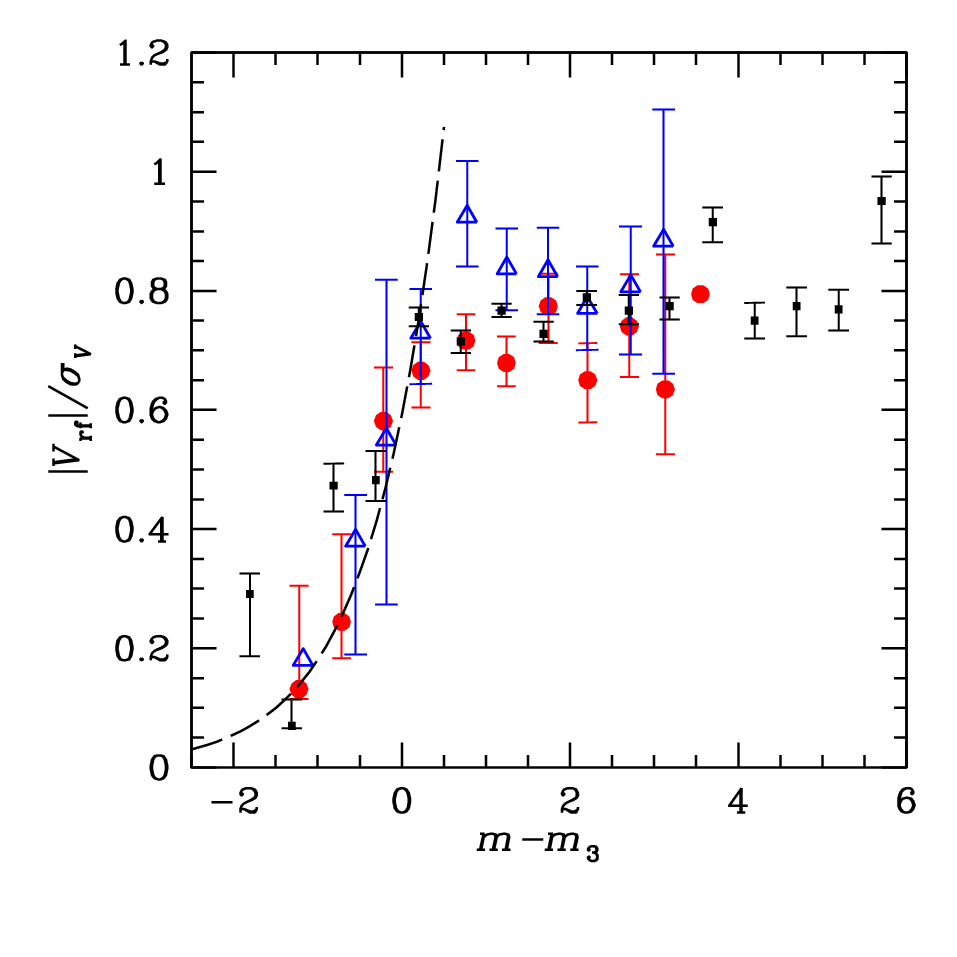
To investigate a possible dependence of VLS with redshift, we also show the results for the three redshift subsamples. Although current data are not sufficient to obtain firm conclusions, the visual inspection of Fig. 10 suggests that the threshold value of segregation in the Low- sample lies at brighter magnitudes than the values in the Medium- and High- samples.

6 Discussion
We find evidence of VCS in our sample of clusters. In our analysis, VCS is detected over the whole sampled galaxy luminosity range (see Fig 9). In particular, analyzing the clusters in three redshift ranges separately, Table 6 shows that the amount of VCS decreases with increasing redshift and that very poor or no evidence of segregation is found in the High- sample. Qualitatively, this is in agreement with the results of Biviano & Poggianti (2009) in EDisCS clusters at -0.8 (our Low-+Medium- samples), for which there is much less evidence of VCS when compared to local clusters. Crawford et al. (2014) found no evidence of VCS between red sequence and blue cloud galaxies in five distant cluster (), but they did not analyze a local sample for comparison.
We confirm that the effect of VCS is quantitatively small and, therefore, difficult to detect. For instance, according to the KS–test, the distributions of red and blue galaxies might derive from the same parent distribution. We had to resort to very sensitive tests such as the S– and W–tests to detect a significant difference in the distributions. Indeed, as most previous positive detections in the literature, our most significant detection is obtained stacking galaxies of all clusters. Quantitatively, the estimates of the difference in reported in the literature are of the order of 10-20%, 30% at most (Biviano et al. 1997; Carlberg et al. 1997; Adami et al. 1998; de Theije & Katgert 1999; Haines et al. 2015) and vary according to the selection of the two populations. In fact, when the population is selected according to higher values of star formation rate, its is higher (Haines et al. 2015). The values we obtained in our study are comparable with those reported in the literature. We estimated that of red and blue galaxies differ for 20% and 10% in the Low- and Medium- samples, and the median value of the ratios of the VDP binned values for blue and red galaxies is 1.2 (within , see Fig. 5).
Taking into account the difficulties related to the detection and measure of VCS, any result is more reliable when obtained through an homogeneous analysis rather than comparing results from different authors. In this context, it is interesting that our results are in line with that of Biviano & Poggianti (2009) on a decreasing amount of VCS at higher redshifts, although their claim holds for clusters at -0.8, while ours for clusters in the range. The poor evidence of VCS in high redshift clusters can be explained in a scenario where the segregation develops as the result of a continuous, regular smooth accretion of field blue galaxies, then possibly evolving in red galaxies, into the cluster. VCS is erased when cluster-cluster mergers drive violent relaxation, and the frequency of such mergers is expected to be higher at higher redshift.
Since our cluster sample spans a large range of masses, of about two orders of magnitudes (see Table 2) we also checked for a possible dependence of VCS with mass. We find no significant correlation of vs the cluster mass. This agrees with the fact that the evidence of VCS, which is well known in clusters, is detected also in groups (Girardi et al. 2003; Ribeiro et al. 2010).
To our knowledge, this is the first study where VLS is detected in non local clusters. The vs relation here detected is similar to that originally shown by Biviano et al. (1992). Assuming the mass-follows-light hypothesis, the faint galaxies can be described by a regime of velocity equipartition, while the bright galaxies can be better described by a regime of energy equipartition, with more massive objects being slower. Since we used red or NIR magnitude bands, the luminosity is a good indicator of the stellar mass, but the mass-follows-light assumption is needed to extrapolate our interpretation to the whole, halo galaxy mass. As already discussed by other authors (Biviano et al. 1992; Mahajan et al. 2011) the most likely cause for the observed VLS is the dynamical friction process, whose characteristic time-scale is inversely proportional to mass.
We confirm that VLS holds for red galaxies and find for the first time evidence that the same segregation also applies to the population of blue galaxies. In fact, both Adami et al. (1998) and Ribeiro et al. (2013) found VLS for ellipticals/passive galaxies, but no (or even opposite) effect is reported for galaxies of other types. However, the inspection of Fig. 2b of Adami et al. (1998) suggests that their non detection might be rather due to the large uncertainties involved. The presence of the VLS for blue galaxies indicates that the kinematical relaxation time-scale is shorter than the transformation time-scale or that massive blue galaxies are robust against environmental effects and possible transformation to S0 (e.g., Moore et al. 1996; Bekki & Couch 2011).
A more detailed comparison of our results with those of Biviano et al. (1992, see also our Fig. 9) shows two differences. As a first difference, our and relation is steeper than their relation. The fit of the logarithm of vs gives a slope of for red galaxies only, and for all galaxies. For comparison, Biviano et al. (1992) obtained a value of 0.2, which is that expected in the case of energy equipartition (assuming a constant mass-to-light ratio). Adami et al. (1998) also claim that a 0.2 slope is consistent with their results, but large uncertainties are shown in their Fig. 1a and the inspection of their Fig. 2a for ellipticals rather suggests a steeper slope. The second difference concerns the threshold value between the two kinematic regimes. Biviano et al. (1992) indicate a threshold value around and Adami et al. (1998) report that VLS concerns about four galaxies per cluster. In the whole sample, our results rather suggest (Fig. 9) and we found that VLS concerns seven galaxies per cluster, computed as the median value of the numbers of galaxies with in each cluster. However, both Biviano et al. (1992) and Adami et al. (1998) analyze local clusters and the inspection of Fig. 10 indicates that the threshold value of VLS in the Low- sample lies at brighter magnitudes than the values in the Medium- and High- samples. Present data do not allow a precise quantitative conclusion, but suggest that the dipendence of the segregation threshold should be taken into account. In particular, the possible explanation for a fainter threshold at higher redshifts might be that clusters at higher redshift have higher density. Per given galaxy mass, the greater the density of the surrounding medium, the stronger the effect of dynamical friction.
7 Summary and conclusions
In this study we present our results about color and luminosity segregation in velocity space (VCS and VLS, resp.) for a sample of 41 clusters at intermediate and high redshifts (), for a total of 4172 galaxies. The data have been taken from different sources in the literature, with the constraint that data for each single cluster come from one single source. Moreover, we applied homogeneous preliminary procedures to select cluster members, compute global cluster properties, in particular the LOS velocity dispersions , and separate blue from red galaxies. We restricted our analysis to the 1674 member galaxies within 2 with photometric or spectroscopic information, 1023 red and 651 blue galaxies. We applied a set of different tests to study VCS and VLS. We used both the estimates of velocity dispersion for each individual cluster and the properties of an ensemble cluster obtained by stacking together galaxies of many clusters.
The main results of our analysis are summarized as follows.
- •
From the analysis of the whole sample we detect evidence of VCS according to several tests (S–, W–, and VDP –tests), with the blue galaxy population having a larger than the red galaxy population.
- •
When analyzing three subsamples at different redshifts (Low- with , Medium- with , High- with ), very poor or no evidence of VCS is found in the High- sample. The fact that VCS is weaker at higher redshifts has been already pointed out by Biviano & Poggianti (2009), although our threshold of no detection is at higher than theirs. The disappearance of the VCS for distant clusters can be explained when considering that our High- sample is very close to the epoch of cluster formation, with major mergers driving violent relaxation which leads to the velocity equipartition regime.
- •
In agreement with previous studies we confirm that the effect of VCS is quantitatively small (10-20% in the estimate) and requires sensitive tests or the VDP analysis based on many galaxies. We conclude that VCS is an elusive effect, that might partly explains the discrepant claims reported in the literature on this issue.
- •
VCS concerns the whole magnitude range that we covered, magnitudes down to ; more clusters are needed to sample the bright end to obtain firm conclusions.
- •
We detect evidence of VLS for galaxies more luminous than , brighter galaxies having lower velocities. Qualitatively, this result is similar to that found for local clusters, but we note and discuss minor differences, e.g. in the threshold value of the segregation.
- •
VLS concerns both red and blue galaxies. The latter finding still not reported in the literature, not even for local clusters.
Finally, we note that there is a strong correlation between based on red galaxies and based on blue galaxies and, in particular, we find no significant bias in the High- sample. Although the appropriate mass calibration has to be determined, this result suggests that both red and blue galaxies can be used as tracers of the cluster mass distribution out to high redshift. This result has interesting implications for the cosmological application of the velocity dispersion measurements that the Euclid satellite will make possible by targeting H-emitting, star-forming galaxies in its spectroscopic survey (Laureijs et al. 2011; Sartoris et al. 2016, e.g.).
Acknowledgements.
We thank the referee for useful comments. We thank P. Rosati for providing us data on XMMU J2235.32557. M.A., and A.B. and M.N. acknowledge financial support from PRIN-INAF 2014 1.05.01.94.02. M.G. acknowledges financial support from the University of Trieste through the program “Finanziamento di Ateneo per progetti di ricerca scientifica - FRA 2015”. S.B. acknowledges financial support from the PRIN-MIUR 201278X4FL grant and from the “InDark” INFN Grant. This research has made use of the NASA/IPAC Extragalactic Database (NED) which is operated by the Jet Propulsion Laboratory, California Institute of Technology, under contract with the National Aeronautics and Space Administration.References
- Abraham et al. (1996) Abraham, R. G., Smecker-Hane, T. A., Hutchings, J. B., et al. 1996, ApJ, 471, 694
- Adami et al. (1998) Adami, C., Biviano, A., & Mazure, A. 1998, A&A, 331, 439
- Ashman et al. (1994) Ashman, K. M., Bird, C. M., & Zepf, S. E. 1994, AJ, 108, 2348
- Beers et al. (1990) Beers, T. C., Flynn, K., & Gebhardt, K. 1990, AJ, 100, 32
- Bekki & Couch (2011) Bekki, K. & Couch, W. J. 2011, MNRAS, 415, 1783
- Biviano et al. (1996) Biviano, A., Durret, F., Gerbal, D., et al. 1996, A&A, 311, 95
- Biviano & Girardi (2003) Biviano, A. & Girardi, M. 2003, ApJ, 585, 205
- Biviano et al. (1992) Biviano, A., Girardi, M., Giuricin, G., Mardirossian, F., & Mezzetti, M. 1992, ApJ, 396, 35
- Biviano & Katgert (2004) Biviano, A. & Katgert, P. 2004, A&A, 424, 779
- Biviano et al. (1997) Biviano, A., Katgert, P., Mazure, A., et al. 1997, A&A, 321, 84
- Biviano et al. (2006) Biviano, A., Murante, G., Borgani, S., et al. 2006, A&A, 456, 23
- Biviano & Poggianti (2009) Biviano, A. & Poggianti, B. M. 2009, A&A, 501, 419
- Biviano et al. (2013) Biviano, A., Rosati, P., Balestra, I., et al. 2013, A&A, 558, A1
- Borgani et al. (1997) Borgani, S., Gardini, A., Girardi, M., & Gottlöber, S. 1997, New A, 2, 119
- Caldwell & Rose (1997) Caldwell, N. & Rose, J. A. 1997, AJ, 113, 492
- Carlberg et al. (1997) Carlberg, R. G., Yee, H. K. C., Ellingson, E., et al. 1997, ApJ, 476, L7
- Carrasco et al. (2007) Carrasco, E. R., Cypriano, E. S., Neto, G. B. L., et al. 2007, ApJ, 664, 777
- Chincarini & Rood (1977) Chincarini, G. & Rood, H. J. 1977, ApJ, 214, 351
- Colless & Dunn (1996) Colless, M. & Dunn, A. M. 1996, ApJ, 458, 435
- Crawford et al. (2014) Crawford, S. M., Wirth, G. D., & Bershady, M. A. 2014, ApJ, 786, 30
- Danese et al. (1980) Danese, L., de Zotti, G., & di Tullio, G. 1980, A&A, 82, 322
- de Theije & Katgert (1999) de Theije, P. A. M. & Katgert, P. 1999, A&A, 341, 371
- Demarco et al. (2010) Demarco, R., Gobat, R., Rosati, P., et al. 2010, ApJ, 725, 1252
- Demarco et al. (2007) Demarco, R., Rosati, P., Lidman, C., et al. 2007, ApJ, 663, 164
- Dolag et al. (2004) Dolag, K., Bartelmann, M., Perrotta, F., et al. 2004, A&A, 416, 853
- Dressler (1980) Dressler, A. 1980, ApJ, 236, 351
- Dressler et al. (1999) Dressler, A., Smail, I., Poggianti, B. M., et al. 1999, ApJS, 122, 51
- Ellingson et al. (1998) Ellingson, E., Yee, H. K. C., Abraham, R. G., Morris, S. L., & Carlberg, R. G. 1998, ApJS, 116, 247
- Ellingson et al. (1997) Ellingson, E., Yee, H. K. C., Abraham, R. G., et al. 1997, ApJS, 113, 1
- Fabricant et al. (1994) Fabricant, D. G., Bautz, M. W., & McClintock, J. E. 1994, AJ, 107, 8
- Fadda et al. (1996) Fadda, D., Girardi, M., Giuricin, G., Mardirossian, F., & Mezzetti, M. 1996, ApJ, 473, 670
- Fassbender et al. (2011) Fassbender, R., Böhringer, H., Santos, J. S., et al. 2011, A&A, 527, A78
- Ferrari et al. (2005) Ferrari, C., Benoist, C., Maurogordato, S., Cappi, A., & Slezak, E. 2005, A&A, 430, 19
- Fukugita et al. (1995) Fukugita, M., Shimasaku, K., & Ichikawa, T. 1995, PASP, 107, 945
- Gerken et al. (2004) Gerken, B., Ziegler, B., Balogh, M., et al. 2004, A&A, 421, 59
- Gioia et al. (1999) Gioia, I. M., Henry, J. P., Mullis, C. R., Ebeling, H., & Wolter, A. 1999, AJ, 117, 2608
- Girardi et al. (1993) Girardi, M., Biviano, A., Giuricin, G., Mardirossian, F., & Mezzetti, M. 1993, ApJ, 404, 38
- Girardi et al. (1996) Girardi, M., Fadda, D., Giuricin, G., et al. 1996, ApJ, 457, 61
- Girardi et al. (2015) Girardi, M., Mercurio, A., Balestra, I., et al. 2015, A&A, 579, A4
- Girardi et al. (2003) Girardi, M., Rigoni, E., Mardirossian, F., & Mezzetti, M. 2003, A&A, 406, 403
- Goto (2005) Goto, T. 2005, MNRAS, 359, 1415
- Haines et al. (2015) Haines, C. P., Pereira, M. J., Smith, G. P., et al. 2015, ApJ, 806, 101
- Halliday et al. (2004) Halliday, C., Milvang-Jensen, B., Poirier, S., et al. 2004, A&A, 427, 397
- Hammer et al. (1997) Hammer, F., Flores, H., Lilly, S. J., et al. 1997, ApJ, 481, 49
- Hernández-Fernández et al. (2014) Hernández-Fernández, J. D., Haines, C. P., Diaferio, A., et al. 2014, MNRAS, 438, 2186
- Hilton et al. (2010) Hilton, M., Lloyd-Davies, E., Stanford, S. A., et al. 2010, ApJ, 718, 133
- Hwang & Lee (2008) Hwang, H. S. & Lee, M. G. 2008, ApJ, 676, 218
- Jørgensen & Chiboucas (2013) Jørgensen, I. & Chiboucas, K. 2013, AJ, 145, 77
- Katgert et al. (1996) Katgert, P., Mazure, A., Perea, J., et al. 1996, A&A, 310, 8
- Laureijs et al. (2011) Laureijs, R., Amiaux, J., Arduini, S., et al. 2011, ArXiv e-prints [arXiv:1110.3193]
- Lederman (1984) Lederman, W. 1984, Handbook of applicable mathematics. Vol.6,A: Statistics; Vol.6,B: Statistics (Wiley-Interscience Publication, Chichester)
- Lerchster et al. (2011) Lerchster, M., Seitz, S., Brimioulle, F., et al. 2011, MNRAS, 411, 2667
- Lubin et al. (2002) Lubin, L. M., Oke, J. B., & Postman, M. 2002, AJ, 124, 1905
- Mahajan et al. (2011) Mahajan, S., Mamon, G. A., & Raychaudhury, S. 2011, MNRAS, 416, 2882
- Melnick & Sargent (1977) Melnick, J. & Sargent, W. L. W. 1977, ApJ, 215, 401
- Milvang-Jensen et al. (2008) Milvang-Jensen, B., Noll, S., Halliday, C., et al. 2008, A&A, 482, 419
- Mohr et al. (1996) Mohr, J. J., Geller, M. J., & Wegner, G. 1996, AJ, 112, 1816
- Moore et al. (1996) Moore, B., Katz, N., Lake, G., Dressler, A., & Oemler, A. 1996, Nature, 379, 613
- Moss & Dickens (1977) Moss, C. & Dickens, R. J. 1977, MNRAS, 178, 701
- Munari et al. (2013) Munari, E., Biviano, A., Borgani, S., Murante, G., & Fabjan, D. 2013, MNRAS, 430, 2638
- Owen et al. (2005) Owen, F. N., Ledlow, M. J., Keel, W. C., Wang, Q. D., & Morrison, G. E. 2005, AJ, 129, 31
- Owers et al. (2011) Owers, M. S., Nulsen, P. E. J., & Couch, W. J. 2011, ApJ, 741, 122
- Pisani (1993) Pisani, A. 1993, MNRAS, 265, 706
- Poggianti (1997) Poggianti, B. M. 1997, A&AS, 122 [astro-ph/9608029]
- Postman et al. (1998) Postman, M., Lubin, L. M., & Oke, J. B. 1998, AJ, 116, 560
- Postman et al. (2001) Postman, M., Lubin, L. M., & Oke, J. B. 2001, AJ, 122, 1125
- Press et al. (1992) Press, W. H., Teukolsky, S. A., Vetterling, W. T., & Flannery, B. P. 1992, Numerical recipes in FORTRAN. The art of scientific computing (Cambridge University Press, Cambridge)
- Ribeiro et al. (2013) Ribeiro, A. L. B., Lopes, P. A. A., & Rembold, S. B. 2013, A&A, 556, A74
- Ribeiro et al. (2010) Ribeiro, A. L. B., Lopes, P. A. A., & Trevisan, M. 2010, MNRAS, 409, L124
- Rines et al. (2013) Rines, K., Geller, M. J., Diaferio, A., & Kurtz, M. J. 2013, ApJ, 767, 15
- Rines et al. (2003) Rines, K., Geller, M. J., Kurtz, M. J., & Diaferio, A. 2003, AJ, 126, 2152
- Rines et al. (2005) Rines, K., Geller, M. J., Kurtz, M. J., & Diaferio, A. 2005, AJ, 130, 1482
- Rosati et al. (2014) Rosati, P., Balestra, I., Grillo, C., et al. 2014, The Messenger, 158, 48
- Rosati et al. (2009) Rosati, P., Tozzi, P., Gobat, R., et al. 2009, A&A, 508, 583
- Santos et al. (2015) Santos, J. S., Altieri, B., Valtchanov, I., et al. 2015, MNRAS, 447, L65
- Sarazin (1986) Sarazin, C. L. 1986, Reviews of Modern Physics, 58, 1
- Sartoris et al. (2016) Sartoris, B., Biviano, A., Fedeli, C., et al. 2016, MNRAS[arXiv:1505.02165]
- Scodeggio et al. (1995) Scodeggio, M., Solanes, J. M., Giovanelli, R., & Haynes, M. P. 1995, ApJ, 444, 41
- Siegel (1956) Siegel, S. 1956, Nonparametric statistics for the behavioral sciences (McGraw-Hill Kogakusha, Tokyo)
- Sodré et al. (1989) Sodré, Jr., L., Capelato, H. V., Steiner, J. E., & Mazure, A. 1989, AJ, 97, 1279
- Tammann (1972) Tammann, G. A. 1972, A&A, 21, 355
- Tanaka et al. (2008) Tanaka, M., Finoguenov, A., Kodama, T., et al. 2008, A&A, 489, 571
- Tran et al. (2007) Tran, K.-V. H., Franx, M., Illingworth, G. D., et al. 2007, ApJ, 661, 750
- Tran et al. (2010) Tran, K.-V. H., Papovich, C., Saintonge, A., et al. 2010, ApJ, 719, L126
- Vulcani et al. (2012) Vulcani, B., Aragón-Salamanca, A., Poggianti, B. M., et al. 2012, A&A, 544, A104
- Westra et al. (2010) Westra, E., Geller, M. J., Kurtz, M. J., Fabricant, D. G., & Dell’Antonio, I. 2010, PASP, 122, 1258
- White et al. (2005) White, S. D. M., Clowe, D. I., Simard, L., et al. 2005, A&A, 444, 365
- Whitmore et al. (1993) Whitmore, B. C., Gilmore, D. M., & Jones, C. 1993, ApJ, 407, 489
- Yee et al. (1996) Yee, H. K. C., Ellingson, E., & Carlberg, R. G. 1996, ApJS, 102, 269
- Zabludoff & Franx (1993) Zabludoff, A. I. & Franx, M. 1993, AJ, 106, 1314
- Ziparo et al. (2014) Ziparo, F., Popesso, P., Finoguenov, A., et al. 2014, MNRAS, 437, 458