Evolution of spherical overdensities in new agegraphic dark energy model
Abstract
We study the structure formation by investigating the spherical collapse model in the context of new agegraphic dark energy model in flat FRW cosmology. We compute the perturbational quantities , , , , , and for the new agegraphic dark energy model and compare the results with those of EdS and models. We find that there is a dark energy dominated universe at low redshifts and a matter dominated universe at high redshifts in agreement with observations. Also, the size of structures, the overdense spherical region, and the halo size in the new agegraphic dark energy model are found smaller, denser, and larger than those of EdS and models. We compare our results with the results of tachyon scalar field and holographic dark energy models.
pacs
98.80.-k; 95.36.+x; 04.50.Kd.I Introduction
The recent accelerated expansion of universe is one of the most significant cosmological discoveries over the last decade [1, 2, 3, 4]. In order to explain this unexpected behavior, many cosmological models have been proposed, some with the basis of modified gravity theories and
some with the basis of dark energy model. The cosmological constant is the
simplest candidate for dark energy but it suffers from cosmic coincidence and fine-tuning problems [5, 6]. The origin and nature of dark energy is still unknown. Thus, many different dark energy models
such as holographic [7], new agegraphic [8],
phantom, quintom [9] and tachyon [10, 11] have been proposed.
We know that the problem of structure formation in the universe is a significant issue in theoretical cosmology. The spherical collapse model presented by Gott and Gunn [12] is
the simplest structure formation model.
In this model, a small spherical region is supposed subject to a homogeneous perturbation which is set in a homogeneous background universe. Also,
in the spherical collapse model, we confront with the important concepts such as virialization and turn-around.
The perturbation grows and quits the linear regime as time passes.
When the radius becomes maximum, the perturbation stops expanding
and the Hubble flow decouples from the homogenous background, this is called turn-around. After this epoch, the perturbation starts
contracting. For a perfect pressureless matter and perfect spherical
symmetry, the perturbation collapses to a single point. However, since there
is hardly any perfect spherical symmetric overdensity in the universe, the
corresponding perturbation does not collapse to a single point. Finally, a virialized object
of a finite size is formed that is called Halo.
In addition, the evolution of structure growth have been investigated in different dark energy models such as: ghost [13], tachyon [14], chaplygin gas [15], holographic [16]
and etc.
In this paper, we study the evolution of the growth
of overdense structures with respect to the dynamics of cosmic redshift or
scale factor. The dynamics of overdense structure depends on the expansion of universe and the dynamics of the background Hubble flow.
The spherical collapse model has been discussed thoroughly in Refs.[17, 18, 19].
In this work, we study the evolution of spherical overdensities in the new agegraphic dark energy model (NADE) and compare our results with the results of EdS and models. Also, we compare our results with the results of tachyon scalar field
model [14] and holographic dark energy model [16].
II cosmology with new agegraphic dark energy model
W know that the cosmological constant suffers from cosmic coincidence and fine-tuning problems known altogether as the cosmological constant problem. In general relativity, the space-time can be measured without any limit of accuracy. However, in quantum mechanics, the Heisenberg uncertainty relation imposes a limit of accuracy in these measurements [8]. Károlyházy and his collaborators [20] constructed an interesting observation about the distance measurement for Minkowski space-time given by
| (1) |
Here is a dimensionless constant of order unity [21, 22]. In this work, we consider , where , and are reduced Planck length, time and mass, respectively. Eq. (1) together with the time-energy uncertainly relation provides the possibility to estimate an energy density of the metric quantum fluctuations of Minkowski space-time [21, 22]. According to [21, 22], with respect to Eq. (1) a length scale can be known with a maximum accuracy determining thereby a minimal detectable cell over a spatial region . Such a cell expresses a minimal detectable unit of space time over a given length scale . If the age of Minkowski space time is , then over a spatial region with linear size there exists a minimal cell , whose energy cannot be smaller than [21, 22]
| (2) |
due to time-energy uncertainly relation. Thus, the energy density of metric quantum fluctuations of Minkowski space-time is given by [21, 22]
| (3) |
With the choice of age of the universe , as the length scale in Eq. (3), one can obtain the agegraphic dark energy model as follows [8]
| (4) |
where is of the order of unity and it is introduced to parameterize some uncertainties such as the effect of curved space-time and the species of quantum fields in the universe. Since this model can not explain the matter dominated era, hence Wei and Cai proposed the new model that is called new agegraphic dark energy model [8]. In Eq. (3), one can choose the time scale to be the conformal time which is defined by . Therefore, the energy density of new agegraphic dark energy is given by [8]
| (5) |
where is of order unity. The conformal time is given by
| (6) |
We consider a flat Friedmann-Robertson-Walker (FRW) universe containing new agegraphic dark energy and pressureless matter. In a flat FRW universe, the Friedmann equation is given by
| (7) |
where , and are the density of new agegraphic dark energy, the pressureless matter density and the Hubble parameter, respectively. We assume that there is no interaction between new agegraphic dark energy and the pressureless matter, thus the continuity equation is given by
| (8) |
| (9) |
The fractional energy densities are also given by
| (10) |
| (11) |
Using Eqs. (5) and (10), we obtain
| (12) |
Taking time derivative of Eq. (5) and using Eqs. (6), (8), (12) and , the new agegraphic dark energy Equation of State parameter (EoS) is obtained
| (13) |
Using , we can write Eq. (13) as follows
| (14) |
Taking time derivative of Eq. (12) and using yields
| (15) |
Similarly, taking time derivative of Eq. (7) and using Eqs. (8), (9), (10) and (11) yields
| (16) |
Now, using Eqs. (14), (16) and inserting Eq. (15), we obtain
| (17) |
Using and Eq.(17), one finds
| (18) |
The evolution of dimensionless Hubble parameter in new agegraphic dark energy model is obtained by using Eqs. (14) and (16) as follows
| (19) |
In figure (1), we have displayed the evolution of Equation of State parameter , the evolution of density parameter and the evolution of dimensionless Hubble parameter E(z) of new agegraphic dark energy model with respect to the redshift parameter z. Also in figure (1), we have assumed the present values: , , and [23].
The evolution of Equation of State parameter
of NADE model with respect to the redshift parameter .

The evolution of density parameter of NADE model with respect to the redshift parameter .

The evolution of dimensionless Hubble parameter in
NADE model
and in the model with respect to the redshift parameter .

III Linear Perturbation Theory
In this section, we discuss the linear perturbation theory of non-relativistic dust matter, , for the new agegraphic dark energy model. Afterwards, we compare the new agegraphic dark energy model with the EdS model and the model. The differential equation for is given by [24, 15, 25]
| (20) |
Using Eqs. (18) and (19), we solve numerically Eq. (20) for studying the linear growth in new agegraphic dark energy model. Then, we compare the linear growth in the new agegraphic dark energy model with the linear growths in the EdS model and the model. Now, we plot the evolution of with respect to a function of the scale factor in figure (2). In the new agegraphic dark energy model, the growth factor evolves more slowly compared to the model because the expansion of the universe slows down the structure formation. Also, in the model, the growth factor evolves more slowly compared to the EdS model because the cosmological constant dominates in the late time universe. These results are similar to the results obtained in the paper Malekjani [16] for holographic dark energy model.

IV Spherical Collapse in the New Agegraphic of Dark Energy Model
The discourse of structure formation is obtained by the differential equation for the evolution of the matter perturbation in a matter dominated universe [26, 27]. The differential equation for the evolution of in a universe including a dark energy component was generalized in [28, 29]. Now, we consider the non- linear differential equation as given by [15]
| (21) |
where ′ defines the derivative with respect to the scale factor . The linear differential equation for the evolution of is given by
| (22) |
Now, in Eqs. (21) and (22) we consider the conditions and for the differential equation of perturbation in the EdS model [15]. In a similar way [15], we obtain the conditions and for the the new agegraphic dark energy and models.
The linear growth of density perturbation in terms of
scale factor for different models

The non-linear growth of density perturbation in terms of scale factor for different models.

Figure (3-a) shows that in the new agegraphic dark energy model the linear growth of density perturbation evolves more slowly compared to the model and in the model, the linear growth of density perturbation evolves more slowly compared to the EdS model. Also, figure (3-b) indicates that the non-linear growth of density perturbation in the new agegraphic dark energy model is faster than that of the EdS model.
V Determination of and
We consider the well known quantities of the spherical collapse model for the new agegraphic dark energy model: is the linear overdensity parameter, the virial overdensity shows the halo size of structure, expresses the overdense spherical area of structure and represents the size structure. Now, we assume a spherical overdense region with matter density in a surrounding universe defined by its background dynamics with density . The virial overdensity is described by [30]
| (23) |
where is the virialization radius and is the scale factor corresponding to virialization. Also, we can rewrite as follows [30]
| (24) |
where
| (25) |
| (26) |
Here, is the turn-around radius and is the scale factor corresponding to the turn-around epoch. Also, we use the virial radius as follows [31]
| (27) |
where
| (28) |
| (29) |
Here, and are the (Wang-Steinhardt) WS parameters. Now, we discuss the results obtained for , , and in the models introduced in this paper.
In the figure (4), we see that in the EdS model, and it is independent of the redshift . In the model, is smaller than 1.686 and its value is approximately the same as that of EdS model at high redshifts. Therefore the universe is matter dominated at high redshift and the cosmological constant dominates at low redshift. We can state that the primary structures form with a lower critical density. Also, in the new agegraphic dark energy model, is smaller than that of model. This is due to the fact that in figure (1c) the Hubble parameter in the new agegraphic dark energy model is larger than that of the model. Hence, there is a dark energy dominated universe at low redshifts and there is a matter dominated universe at high redshifts.
In the figure (5), we see that in the EdS model, and it is independent of the redshift . In the model, is smaller than 0.5 and its value is approximately the same as that of EdS model at high redshifts . Also, in the new agegraphic dark energy model, is smaller than that of model. Thus, we find that the size of structures in the new agegraphic dark energy model is smaller than that of the model.

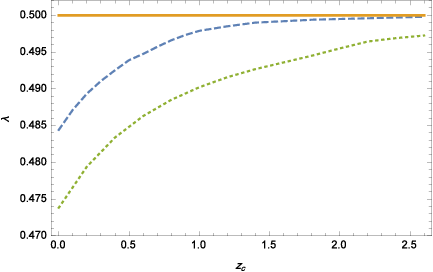
The variation of for the NADE model, the model and the EdS model.

The variation of for the
NADE model, the model and the EdS model.

In the figure (6a), we see that in the EdS model, and it is independent of the redshift . In the model, is larger than 5.6 but its value is approximately the same as that of EdS model at high redshifts. Also, in the new agegraphic dark energy model, is larger than the model. Thus, we find that in the new agegraphic dark energy model, the overdense spherical area is denser than the EdS model and the model.
In the figure (6b), we see that in the EdS model, and it is independent of the redshift . In the model, is larger than 178 but its value is approximately the same as that of EdS model at high redshifts. Also, in the new agegraphic dark energy model, value is larger than the model. Thus, we find that in the new agegraphic dark energy model, the halo size is larger than those of EdS and models.
VI mass function and number density
In this section, we calculate the number density and the mass function in a given mass range. The average comoving number density of halos of mass is described by [32, 33]
| (30) |
Here, is the background density and is the multiplicity function. Also, is described by
| (31) |
where is the r.m.s of the mass fluctuation in the sphere of mass M. The formula is given by [34]
| (32) |
Here, and are the mass variance of the overdensity on the scale of and mass inside a sphere, respectively. is the radius inside a sphere. The numerical values and are and , respectively. The formula is given by [34]
| (33) |
where is the linear growth factor. The formula is given by
| (34) |
The formula is described by
| (35) |
where
| (36) |
Eqs. (32), (33) and (34) have validity limits [34]. They represent that the fitting formula predicts lower values of the values of the variance for and the fitting formula predicts higher values of the values of the variance for . Now, we can use the ST mass function formula given by [35, 36]
| (37) |
Here the numerical parameters are: , and . Also, we use the PO mass function formula given by [37, 38]
| (38) |
where the numerical parameter is: . The YNY mass function formula is presented by [39]
| (39) |
where the numerical parameters are: , , and .
The evolution of the mass function for the new agegraphic dark energy and the models in the case .

The evolution of the mass function
for the NADE model and the model in the case .

The evolution of the number density
for NADE model and the model in the case .

The evolution of the number density for the new agegraphic dark energy model and the model in the case .


Now, we discuss the evolution of the ST mass function with represent to for the new agegraphic dark energy model and the model in the figure (7). The formula is defined as . In the figure (7), the evolution of the ST mass function with represent to is identical for the new agegraphic dark energy model and the model in the case, but it is different for the new agegraphic dark energy model and the model in the case. This difference is due to the difference between and in two models. Also, and are dependent on the redshift. Using Eqs. (30) and (37), we obtain the average comoving number density of halos of mass for the new agegraphic dark energy model and the model in the and cases. In the figure (8), the evolution of the number density with represent to is identical to those of the new agegraphic dark energy model and the model in the case, but it is different for the new agegraphic dark energy model and the model in the case. In the figure (8b), for small objects the difference in the number densities of halo objects is low but the difference in the number densities of halo objects is increasing for high mass in the new agegraphic dark energy model and the model. Therefore, we find that the number of objects per unit mass is increasing for high mass in the new agegraphic dark energy model and the model. Now, using Eqs. (37), (38) and (39), we compare the various mass functions at in figure (9). We can see that the PO mass function is larger than YNY mass function and ST mass function, for all mass scales.
VII Comparison between the new agegraphic dark energy model with the tachyon scalar field and the holographic dark energy models
In this section, we express the results of the evolution of spherical overdensities in new agegraphic dark energy model and compare our results with the results of the tachyon scalar field model (for all ) [14] and the holographic dark energy model (only for )[16].
In the new agegraphic dark energy model, the growth factor evolves more slowly compared to the model because the expansion of the universe slows down the structure formation. Also, in the model, the growth factor evolves more slowly compared to the EdS model because the cosmological constant dominates in the late time universe. In the tachyon scalar field model, at the beginning, the growth factor is larger than the EdS and the models for small scale factors, but for larger scale factors, its growth factor is smaller than the EdS model while it is still larger than the model. Therefore, at first, the tachyon scalar field model predicts the structure formation more impressive than the EdS and the models and over time, the structure formation in the tachyon scalar field model coincides with the EdS and the models [14]. The structure formation in the holographic dark energy model is similar to the new agegraphic dark energy model [16].
In the new agegraphic dark energy model, the linear overdensity parameter is larger than the linear overdensity parameters in the tachyon scalar field model and the holographic dark energy model, respectively. This means that the Hubble parameter in the new agegraphic dark energy model is smaller than the hubble parameter in the tachyon scalar field model and the holographic dark energy model, respectively.
We may compare for the new agegraphic dark energy model, the tachyon scalar field model and the holographic dark energy model. We find that the size of structures in the holographic dark energy model is larger than those of the new agegraphic dark energy and the tachyon scalar field models.
Also, we can conclude that in the tachyon scalar field model, is denser than the new agegraphic dark energy model and the holographic dark energy model, respectively. We can also claim that in the tachyon scalar field model, the halo size is larger than those of the new agegraphic dark energy model and the holographic dark energy model.
Finally, we discuss the evolution of the ST mass function with represent to for the new agegraphic dark energy model, the tachyon scalar field model and the holographic dark energy model in the and cases. The evolution of the ST mass function with represent to is the same for the three models described above in the case but it is different from them in the case. Therefore, the evolution of the ST mass function in the new agegraphic dark energy model is smaller than those of the holographic and the tachyon dark energy models in the z=1 case, respectively.
Also, we compare the average comoving number density of halos of mass for the new agegraphic, the tachyon and the holographic dark energy models in the and cases. We can claim that the evolution of the number density with represent to is identical for the new agegraphic, the tachyon and the holographic dark energy models in the case, but it is different from them in the case. The evolution of the number density in the new agegraphic dark energy model is smaller than those of the holographic and the tachyon dark energy models in the case. Thus, we can claim that the number of objects per unit mass increases for high mass in the new agegraphic, the holographic and the tachyon dark energy models, respectively. We compare the various mass functions at for the new agegraphic, the tachyon and the holographic dark energy models in the . We can see that the PO mass function is larger than YNY mass function and ST mass function for the three models described above.
VIII Concluding remarks
In this work, we discussed the evolution of spherical overdensities in the new agegraphic dark energy model. We obtained the evolution of the dimensionless Hubble parameter , the evolution of density parameter and the evolution of the equation of state parameter for the new agegraphic dark energy model with respect to the cosmic redshift function. We compared the linear growth in the new agegraphic dark energy model with the linear growth in the EdS model and the model: In the new agegraphic dark energy model, the growth factor evolves more slowly compared to the model because the expansion of the universe slows down the structure formation. Also, in the model, the growth factor evolves more slowly compared to the EdS model because the cosmological constant dominates in the late time universe.
We showed that in the EdS model, is independent of the redshift and in the new agegraphic dark energy model, is smaller than that of the model because in figure (1c) the Hubble parameter in the new agegraphic dark energy model is larger than that of the model. Hence, there is a dark energy dominated universe at low redshifts and there is a matter dominated universe at high redshifts.
We saw that in the EdS model, is independent of the redshift and the size of structures in the new agegraphic dark energy model is smaller than that of the model. Also, we concluded that in the EdS model, is independent of the redshift and the overdense spherical area in the new agegraphic dark energy model is denser than those of the EdS model and the model. We found that in the EdS model, is independent of the redshift and in the new agegraphic dark energy model the halo size is larger than those of the EdS model and the model.
Finally, we discussed the evolution of the ST mass function with represent to for the new agegraphic dark energy model and the model. We saw that the evolution of the ST mass function with represent to is identical to the new agegraphic dark energy model and the model in the case, but it is different from the new agegraphic dark energy model and the model in the case. We studied the average comoving number density of halos of mass for the new agegraphic dark energy model and the model in the and cases . We saw that the evolution of the number density with represent to is identical for the new agegraphic dark energy model and the model in the case, but it is different from the new agegraphic dark energy model and the model in the case. In the figure (8b), for small objects the difference in the number densities of halo objects is low but the difference in the number densities of halo objects is increasing for high mass in the new agegraphic dark energy model and the model. Therefore, we found that the number of objects per unit mass is increasing for high mass in the new agegraphic dark energy model and the model. Moreover, we compared the results of the evolution of spherical overdensities in the new agegraphic dark energy model with the results of the tachyon scalar field model (for all n) [14] and the holographic dark energy model (only for ) [16].
References
- [1] A. G. Riess, et al., Astron. J. 116, 1099 (1998).
- [2] S. perlmutter , et al., Astrophys. J. 517, 565 (1999).
- [3] P. De Bernardis, Et al., Nature 404, 955 (2000).
- [4] S. perlmutter , et al., Astrophys. J. 598, 102 (2003); U. Seljak, et al., Phys. Rev. D 71, 103515 (2005).
- [5] S. Weinberg, Rev. Modern. Phys. 61, 1 (1989).
- [6] E. J. Copeland, M. Sami, S. Tsujikawa, 15, 1753 (2006).
- [7] M. Li, Phys. Lett. B 603, 1 (2004).
- [8] H. Wei, R. G. Cai, Phys. Lett. B 660, 113 (2008).
- [9] Y. F. Cai, E. N. Saridakis, M. R. Setare, J. Q. Xia, Phys. Rept. 493, 1 (2010).
- [10] M. R. Setare, Phys. Lett. B 653, 116 (2007).
- [11] M. R. Setare, J. Sadeghi, A. R. Amani, Phys. Lett. B 673, 241 (2009).
- [12] J. E. Gunn, R. J. Gott, ApJ, 176, 1 (1972).
- [13] M. Malekjani, T. Naderi, F. Pace, MNRAS 453, 4148 (2015).
- [14] M. R. Setare, F. Felegary, F. Darabi, arXiv:1607.05318.
- [15] F. Pace, J. C. Waizmann, M. Bartelmann, MNRAS, 406, 1865 (2010).
- [16] T. Naderi, M. Malekjani, F. Pace, MNRAS, 447, 1873 (2015).
- [17] A. J. Fillmore, P. Goldreich, ApJ, 281, 1 (1984).
- [18] Y. Hoffman, J. Shaham, ApJ. 297, 16 (1985).
- [19] S. B. Ryden, E. J. Gunn, ApJ. 318, 15 (1987).
- [20]
F. Károlyházy, Nuovo Cim. A 42, 390 (1966);
F. Károlyházy, A. Frenkel, B. Lukács, in Quantum Concepts in Space and Time, Clarendon Press, oxford, MA (1986); F. Károlyházy, A. Frenkel, B. Lukács, in Physics az Natural Philosophy, MIT Press, Cambridge, MA (1982). - [21] M. Maziashvili, Int. J. Mod. Phys. D 16, 1531 (2007).
- [22] M. Maziashvili, Phys. Lett. B 652, 165 (2007).
- [23] H. Wei, R. G. Cai, Phys. Lett. B 663, 1 (2008).
- [24] W. J. Percival, A. A. 443, 819 (2005).
- [25] F. Pace, L. Moscardi, R. Crittenden, M. Bartelmann, V. Pettorino, MNRAS, 437, 547 (2014).
- [26] F. Bernardeau, ApJ, 433, 1 (1994).
- [27] T. Padmanabhan, Cosmology and Astrophysics through Problems, Cambridge University Press (1996).
- [28] L. R. Abramo, R. C. Batista, L. Liberato, R. Rosenfeld, JCAP, 11, 12 (2007).
- [29]
L. R. Abramo, R. C. Batista, L. Liberato, R. Rosenfeld, Phys. Rev. D 77, 067301 (2008);
L. R. Abramo, R. C. Batista, L. Liberato, R. Rosenfeld, Phys. Rev. D 79, 023516 (2009);
L. R. Abramo, R. C. Batista,, R. Rosenfeld, J. Cosmol. Astropart. Phys, 7, 40 (2009). - [30] S. Meyer, F. Pace, M. Bartelmann, Phys. Rev. D 86, 103002 (2012).
- [31] L. Wang, P. J. Steinhardt, Astro. Phys. J. 508, 483 (1998).
- [32] H. W. Press, P. Schechter, ApJ, 187, 425 (1974).
- [33] R. J. Bond, S. Cole, G. Efstathiou, N. Kaiser, ApJ, 374, 440 (1991).
- [34] P. T. P. Viana, A. R. Liddle, MNRAS, 281, 323 (1996).
- [35] R. K. Sheth, G. Tormen, MNRAS, 308, 119 (1999).
- [36] R. K. Sheth, G. Tormen, MNRAS, 329, 61 (2002).
- [37] A. del Popolo, ApJ, 637, 12 (2006).
- [38] A. del Popolo, A. A, 448, 439 (2006).
- [39] H. Yahagi, M. Nagashima, Y. Yoshii, ApJ, 605, 709 (2004).