Sub-dominant cogrowth behaviour and the viability of deciding amenability numericallyThanks: Research supported by Australian Research Council grant FT110100178
Abstract.
We critically analyse a recent numerical method due to the first author, Rechnitzer and van Rensburg, which attempts to detect amenability or non-amenability in a finitely generated group by numerically estimating its asymptotic cogrowth rate. We identify two potential sources of error. We then propose a modification of the method that enables it to easily compute surprisingly accurate estimates for initial terms of the cogrowth sequence.
Key words and phrases:
amenable group; cogrowth function; Følner function; Kesten’s criterion; return probability; Metropolis algorithm; R. Thompson’s group2010 Mathematics Subject Classification
20F69, 20F65, 05A15, 60J201. Introduction
Researchers studying the amenability Thompson’s group will be familiar with a distrust of experimental methods applied to this problem. Part of this scepticism stems from the fact that (if it is amenable) is known to have a very quickly growing Følner function [22]. However, experimental algorithms investigating amenability are rarely based on Følner’s criteria directly, and to date no identification is made in the literature of a mechanism by which a quickly growing Følner function could interfere with a given experimental method.
In this paper we identify such a mechanism for a recent algorithm proposed by first author, A. Rechnitzer, and E. J. Janse van Rensburg [9], which was designed to experimentally detect amenability via the Grigorchuk-Cohen characterisation in terms of the cogrowth function. We will refer to this as the ERR algorithm in the sequel.
We show that, in the ERR algorithm, estimates of the asymptotic cogrowth rate are compromised by sub-dominant behaviour in the reduced-cogrowth function.
However, even though sub-dominant behaviour in the cogrowth function may interfere with estimates of the asymptotic growth rate, the ERR algorithm can still be used to estimate other properties of the cogrowth function to high levels of accuracy. In particular we are able re-purpose the algorithm to quickly estimate initial values of the cogrowth function even for groups for which the determination of the asymptotic growth rate is not possible (for example groups with unsolvable word problem).
The present work started out as an independent verification by the second author of the experimental results in [9], as part of his PhD research. More details can be found in [27].
The article is organised as follows. In Section 2 we give the necessary background on amenability, random walks and cogrowth, followed by a summary of previous experimental work on the amenability of . In Section 3 a function quantifying the sub-dominant properties of the reduced-cogrowth function is defined. In Section 4 the ERR algorithm is summarised, followed by an analysis of two types of pathological behaviour in Section 5. The first of these is easily handled, while the second is shown to depend on sub-dominant terms in the reduced-cogrowth function. In Section 6 the ERR method is modified to provide estimates of initial cogrowth values. Using this the first 2000 terms for the cogrowth function of Thompson’s group are estimated.
2. Preliminaries
We begin with a definition of terms and a quick survey of experimental work done on estimating amenability.
2.1. Characterisations of amenability
The following characterisation of amenability is due to Grigorchuk [15] and Cohen [8]. A shorter proof of the equivalence of this criteria with amenability was provided by Szwarc [28].
Definition 2.1.
Let be a finitely generated non-free group with symmetric generating set . Let denote the number of freely reduced words of length over which are equal to the identity in . Then is amenable if and only if
Equivalently, let denote the number of words (reduced and unreduced) of length over which are equal to the identity. Then is amenable if and only if
The function is called the reduced-cogrowth function for with respect to , and the cogrowth function.
Kesten’s criteria for amenability is given in terms of the probability of a random walk on the group returning to its starting point.
Definition 2.2.
Let be a finitely generated group, and let be a symmetric measure on . The random walk motivated by is a Markov chain on the group starting at the identity where the probability of moving from to is . Note the distribution after steps is given by the -fold convolution power of , which we denote as . That is, is the probability that an -step walk starting at ends at . By Kesten’s criteria [18] a group is amenable if and only if
Pittet and Saloff-Coste proved that the asymptotic decay rate of the probability of return function is independent of measure chosen, up to the usual equivalence [24]. For finitely generated groups we can choose the random walk motivated by the uniform probability measure on a finite generating set. This random walk is called a simple random walk and corresponds exactly with a random walk on the Cayley graph. For this measure the probability of return is given by
| (1) |
where the (reduced and non-reduced) cogrowth terms are calculated with respect to the support of the measure. Thus the cogrowth function arises from a special case of return probabilities.
Følner’s characterisation of amenability [13] can be phrased in several ways. Here we give the definition for finitely generated groups.
Definition 2.3.
Let be a group with finite generating set . For each finite subset , we denote by the number of elements in . The boundary of a finite set is defined to be
A finitely generated group is amenable if and only if there exists a sequence of finite subsets such that
Vershik [29] defined the following function as a way to quantify how much of the Cayley graph must be considered before sets with a given isoperimetric profile can be found.
Definition 2.4.
The Følner function of a group is
Significant literature exists on Følner functions. It is known that there exists finitely presented amenable groups with Følner functions growing faster than ([20] Corollary 6.3) and finitely generated groups (iterated wreath product of copies of ) with Følner functions growing faster than of height for arbitrary [11].
2.2. Experimental work on the amenability of
Richard Thompson’s group is the group with presentation
| (2) |
where denotes the commutator of two elements. See for example [6] for a more detailed introduction to this group.
Whether or not is amenable has attracted a large amount of interest, and has so far evaded many different attempts at a proof of both positive and negative answers.
The following is a short summary of experimental work previously done on Thompson’s group .
- [5]
Burillo, Cleary and Wiest 2007. The authors randomly choose words and reduce them to a normal form to test if they represent the identity element. From this they estimate the proportion of words of length equal to the identity, as a way to compute the asymptotic growth rate of the cogrowth function.
- [1]
Arzhantseva, Guba, Lustig, and Préaux 2008. The authors study the density or least upper bound for the average vertex degree of any finite subgraph of the Cayley graph; an -generated group is amenable if and only if the density of the corresponding Cayley graph is (considering inverse edges as distinct). A computer program is run and data is collected on a range of amenable and non-amenable groups. They find a finite subset in with density with respect to the generator presentation above. (To be amenable one would need to find sets whose density approaches ). Subsequent theoretical work of Belk and Brown gives sets with density approaching [2].
- [10]
Elder, Rechnitzer and Wong 2012. Lower bounds on the cogrowth rates of various groups are obtained by computing the dominant eigenvalue of the adjacency matrix of truncated Cayley graphs. These bounds are extrapolated to estimate the cogrowth rate. As a byproduct the first 22 coefficients of the cogrowth series are computed exactly.
- [17]
Haagerup, Haagerup, and Ramirez-Solano 2015. Precise lower bounds of certain norms of elements in the group ring of are computed, and coefficients of the first 48 terms of the cogrowth series are computed exactly.
- [9]
Elder, Rechnitzer and van Rensburg 2015. The Metropolis Monte Carlo method from statistical mechanics is adapted to estimate the asymptotic growth rate of the cogrowth function by running random walks on the set of all trivial words in a group. The results obtained for Thompson’s group suggest it to be non-amenable. We describe their method in more detail in Section 4 below.
Justin Moore [22] (2013) has shown that if were amenable then its Følner function would increase faster than a tower of twos,
This result has been proposed as an obstruction to all computational methods for approximating amenability; a computationally infeasibly large portion of the Cayley graph must be considered before sets with small boundaries can be found. However, in all but one of the experimental algorithms listed above computing Følner sets was not the principle aim. In order to understand how a bad Følner function affects the performance of these methods, we need to understand the connection between convergence properties of the respective limits in the various characterisations of amenability.
3. Quantifying sub-dominant cogrowth behaviour
The Følner function quantifies the rate of convergence of the limit in Definition 2.3. We consider the following definitions as an attempt to quantify the rate of convergence of the limits in Definition 2.1.
Definition 3.1.
Let be a finitely generated group with symmetric generating set . Let be the number of all reduced trivial words of length and let Define
Definition 3.1 uses only even word lengths (and hence instead of ). This is necessary because group presentations with only even length relators have no odd length trivial words. For this paper we will only consider the function for amenable groups, in which case except when the group is free (infinite cyclic).
A similar definition may be made for the cogrowth function.
Definition 3.2.
For a finitely generated group with symmetric generating set we may define
where be the number of all (reduced and non-reduced) trivial words of length and
Literature already exists studying the convergence properties of return probabilities, and we suspect that the function is a reformulation of the -isoperimetric function [3].
Example 3.3.
For the trivial group with some finite symmetric generating set we have for so and . Similarly since we have .
Aside from the trivial group, it is usually easier to compute (or its asymptotics) than it is to obtain . For this reason we first consider functions for various groups, and then prove that for infinite, amenable, non-free groups and have the same asymptotic behaviour.
Example 3.4.
For any finite group the rate of growth of is the dominant eigenvalue of the adjacency matrix of the Cayley graph, and some simple analysis shows that is at most logarithmic in .
Define if there exist constants , such that for large enough, . Then ( and are asymptotic) if and .
Table 1 provides a sample of amenable groups for which the asymptotics of , the Følner function and probabilities of return are known [11, 25, 26].
| Example | |||
|---|---|---|---|
| trivial | constant | constant | constant |
| -fold wreath product | (tower of ’s) |
The results for the asymptotics of were derived directly from the known asymptotics for . A discussion of these methods will appear in [27]. In practice however it proved quicker to guess the asymptotics and then refine using the following method.
Proposition 3.5.
The asymptotic results for in Table 1 are correct.
Proof.
For a given group suppose where is a continuous real valued function, as in Table 1. Then .
Finding requires solving the equation
| (3) |
for . This is equivalent to solving
for .
Suppose is a function where
| (4) |
exists and is non-zero.
If exists and is non-zero then
Then
and so .
3.1. Converting from cogrowth to reduced-cogrowth
We now prove an equivalence between the sub-dominant behaviour of the cogrowth and reduced-cogrowth functions. This allows us to borrow the previously listed results for when discussing and the ERR method. The dominant and sub-dominant cogrowth behaviour can be analysed from the generating functions for these sequences.
Definition 3.6.
Let denote the number of trivial words of length in a finitely generated group. The cogrowth series is defined to be
Let denote the number of reduced trivial words. Then
is said to be the reduced-cogrowth series.
and are the generating functions for and respectively, and are related in the following way. Let be the size of a symmetric generating set. Then from [19, 30]
| (5) |
and
| (6) |
The dominant and sub-dominant growth properties of the cogrowth functions may be analysed by considering the singularities of these generating functions. For a detailed study of the relationship between singularities of generating functions and sub-dominant behaviours of coefficients see [12].
We now outline an example of how the composition of functions (as in Equations 5 and 6) effects the growth properties of the series coefficients.
Example 3.7.
Consider
Then (for positive ) has a singularity at , and this defines the radius of convergence of and the asymptotic growth rate of the series coefficients of the expansion of . It also determines the principle sub-dominant term contributing to the growth of the coefficients. In this example, the coefficients will grow like
We wish to investigate what happens to this growth behaviour when we compose the function with a function . Consider for some function for which . The singularities of are inherited by ; if is analytic everywhere then the only singularities of will occur when . In this case, the new radius of convergence will be the minimum such that . Importantly, however, the principle sub-dominant growth term of the series coefficients will remain polynomial of degree .
A variation on this behaviour will occur if there is an for which is analytic on the ball of radius , and for some in this region. Again, when this occurs, the new radius of convergence is obtained by solving and the type of the principle sub-dominant term in the growth of the coefficients remains unchanged.
If there does not exist such an , the principle singularity of will dominate the growth properties of the coefficients.
Proposition 3.8.
Let be an infinite amenable group generated by elements and their inverses. Then the principle sub-dominant terms contributing to the growth of and are asymptotically equivalent, except when the group is infinite cyclic.
Proof.
For an amenable group generated by elements and their inverses the radius of convergence for is exactly . This follows immediately from Definition 2.1.
Now from Equation 5, the reduced-cogrowth series is obtained by composing the cogrowth series with
and then multiplying by
Both of these functions are analytic inside the ball of radius .
Now
| (7) |
the singularity of . Hence, is a singularity of , and hence of . Note that if the group is infinite cyclic, then and and are equal. In this scenario the radius of convergence of is reached at the same moment that reaches the radius of convergence of . This means that both and contribute to the principle singularity, and this explains why the reduced and non-reduced cogrowth functions for the infinite cyclic group exhibit such different behaviour.
If then is inside the ball of radius (ie, inside the region of convergence for and ). Thus, the singularity of is reached before approaches the singularity of and
In this case the substitutions in Equation 5 change the location of the principle singularity, but do not change the type of the singularity, or the form of the principle sub-dominant term contributing to the growth of the series coefficients. ∎
Corollary 3.9.
Suppose is a finitely generated, infinite amenable group that is not the infinite cyclic group. Then is asymptotically equivalent to .
Remark 3.10.
An alternate proof of the Grigorchuk/Cohen characterisation of amenability is easily constructed from an analysis of the singularities of and . For example, Equation 7 proves the first result from Definition 2.1. This argument also picks up that the infinite cyclic group presents a special case. Though amenable, . For this group we have while .
3.2. Sub-dominant behaviour in the cogrowth of
The groups limit to in the space of marked groups. This implies that the growth of the function and hence for increases with . This is consistent with Table 1, since these results do not include scaling constants. This leads to the following result.
Proposition 3.11.
If Thompson’s group is amenable, its function grows faster than the function for any . In particular, it is asymptotically super-polynomial.
Proof.
By the convergence of to in the space of marked groups we have that, for any , the function for grows slower than the corresponding function for . In [24] it is proved that, for finitely generated groups, the probability of return cannot asymptotically exceed the probability of return of any finitely generated subgroup. This implies that, for finitely generated amenable groups, the function of the group must grow faster than the function of any finitely generated subgroup. Since there is a subgroup of isomorphic to , for must grow faster than for and hence .
Since contains every finite depth iterated wreath products of ([16] Corollary 20), the probability of return for decays faster than
for any . Taking the limit as approaches infinity of the corresponding values for and then doing the conversion from to gives the final result. ∎
Note that if is non-amenable, then even though it still contains these subgroups, they do not affect the function. In this scenario it is still true that the return probability for decays faster than the interated wreath product, because would have exponentially decaying return probability. For non-amenable groups the return probability does not identify the principle sub-dominant term in , and hence does not correlate directly with .
4. The ERR algorithm
We start by summarising the original work by the first author, Rechnitzer and van Rensburg. Only the details directly pertinent to the present paper are discussed here, for a more detailed analysis of the random walk algorithm and a derivation of the stationary distribution we refer the reader to [9]. For the sake of brevity the random walk performed by the algorithm will be referred to as the ERR random walk.
Recall that a group presentation, denoted , consists of a set of formal symbols (the generators) and a set of words written in (the relators) and corresponds to the quotient of the free group on by the normal closure of the relators . In our paper, as in [9], all groups will be finitely presented: both and will be finite. Furthermore, the implementation of the algorithm assumes both and to be symmetric, that is, and . In addition, for convenience is enlarged to be closed under cyclic permutation. Recall that counts the number of reduced words in of length which represent the identity in the group (that is, belong to the normal closure of in the free group).
4.1. The ERR random walk
The ERR random walk is not a random walk on the Cayley graph of a group, but instead a random walk on the set of trivial words for the group presentation. This makes the algorithm extremely easy to implement, since it does not require an easily computable normal form or even a solution to the word problem. The walk begins at the empty word, and constructs new trivial words from the current trivial word using one of two moves:
- •
(conjugation by ). In this move an element is chosen from according to a predetermined probability distribution. The current word is conjugated by the chosen generator and then freely reduced to produce the new candidate word.
- •
(insertion of a relator). In this move a relator is chosen from according to a predetermined distribution and inserted into the current word at a position chosen uniformly at random . In order to maintain the detailed balance criteria (from which the stationary distribution is derived) it is necessary to allow only those insertions which can be immediately reversed by inserting the inverse of the relator at the same position. To this end the a notion of left insertion is introduced; after relators are inserted free reduction is done on only the left hand side of the relator. If after this the word is not freely reduced the move is rejected.
Transition probabilities are defined which determine whether or not the trivial word created with these moves is accepted as the new state. These probabilities involve parameters and which may be adjusted to control the distribution of the walk.
Let the current word be and the candidate word be .
- •
If was obtained from via a conjugation it is accepted as the new current state with probability
- •
If was obtained from via an insertion it is accepted as the new state with probability
If is not accepted the new state remains as .
These probabilities are chosen so that the distribution on the set of all trivial words given by
(where is a normalizing constant) can be proved to be the unique stationary distribution of the Markov chain, and the limiting distribution of the random walk.
The following result is then given.
Proposition 4.1 ([9]).
As approaches
the expected value of the word lengths visited approaches infinity.
This result leads to the following method for estimating the value of . For each presentation, random walks are run with different values of . Average word length is plotted against . The results obtained for Thompson’s group are reproduced in Figure 1. The values for at which the data points diverge gives an indication of , and hence the amenability or otherwise of the group.
Random walks were run on presentations for a selection of amenable and non-amenable groups, including Baumslag-Solitar groups, some free product examples whose cogrowth series are known [21], the genus 2 hyperbolic surface group, a finitely presented group related to the basilica group, and Thompson’s group .
The data in Figure 1 appears to show fairly convincingly that the location of is a long way from the value of expected were the group amenable.
It is noted in [9] that a long random walk may be split into shorter segments, and the variation in average word lengths of the segments gives an estimation of the error in the estimated expected word length.
Remark 4.2.
In the original work reported in [9], the algorithm was coded in c++, words were stored as linked lists, the GNU Scientific Library was used to generate pseudo-random numbers, and parallel tempering was used to speed up the convergence of the random walk. For independent verification the second author coded the algorithm in python, kept words as strings, used the python package random, and no tempering was used. Results obtained were consistent with those in [9]. The experimental analysis and modifications described in this paper use the python version of the second author.
5. Investigating Pathological Behaviour
The theory underpinning the ERR random walk is complete — the random walk is certain to converge to the stationary distribution. This does not preclude, however, convergence happening at a computationally indetectible rate. Since there are finitely presented groups with unsolvable word problem, there is no chance of deriving bounds on the rates of convergence of the walk in any generality. In the process of independently verifying the results in [9], however, we were able to identify two properties of group presentations which appear to slow the rate of convergence. The first of these is unconnected with the Følner function, and does not pose any problem to the implementation of the ERR algorithm to Thompson’s group . It does, however, refute the claim in ([9] Section 3.7) that the method can be successfully applied to infinite presentations.
5.1. Walking on the wrong group
It is easy to see from the probabilistic selection criteria used by the ERR random walk that moves which increase the word length by a large amount are rejected with high probability. This poses a problem for group presentations containing long relators since insertion moves that attempt to insert a long relator will be accepted much less often than moves which attempt to insert a shorter relation.
The following example makes this explicit.
Lemma 5.1.
All presentations of the form
describe the trivial group.
Proof.
Since we have
Since we have so .
Putting these results together gives and hence is trivial. The result follows. ∎
By increasing we can make the second relator arbitrarily large without affecting the group represented by the presentation, or the group elements represented by the generators. This implies that ERR random walks for each of these presentations should converge to the same stationary distribution.
Changing the presentation, however, does change the number of steps in the ERR random walk needed to reach certain trivial words (such as the word ‘’).
ERR random walks were performed on these presentations for . As well as recording the average word length of words visited, the number of accepted insertions of each relator was recorded.
| number of steps | number of accepted insertions of small relator | number of accepted insertions for big relator | |
| 1 | |||
| 2 | |||
| 3 | |||
| 4 | |||
| 5 | |||
| 6 | |||
| 7 | |||
| 8 | |||
| 9 | |||
| 10 | |||
| 11 | |||
| 12 | |||
| 13 | |||
| 14 | |||
| 15 | |||
| 16 | |||
| 17 | |||
| 18 | |||
| 19 |
Table 2 shows the sharp decline in the number of accepted insertions of the second relator as increases. Indeed, for there were no instances in which the longer relator was successfully inserted. Unsurprisingly, walks for large did not converge to the same distribution as those where was small, and for large the data did not accurately predict the asymptotic growth rate of the cogrowth function. For these the ERR random walk was actually taking place on , which is a presentation for the 3-stand braid group, which is non-amenable.
Note that, given enough time, the longer relator would be successfully sampled, and that an infinite random walk is still guaranteed to converge to the theoretical distribution for the trivial group. Such convergence, however, may take a computationally infeasible amount of time.
Claim 5.2.
The presence of long relators in the input presentation slows the rate at which an ERR random walk converges to the stationary distribution. Therefore, the ERR method cannot be reliably extended to accept infinite presentations.
This result is not surprising. In [4] an infinitely presented amenable group is given for which any truncated presentation (removing all but a finite number of relators) is non-amenable. The ERR method could not expect to succeed on this group even if long relators were sampled often; since the ERR random walk can only be run for a finite time there can never be a representative sampling of an infinite set of relators, so ERR would incorrectly conclude this group is non-amenable.
The pathological presentations of the trivial group studied here form a sequence of presentations for amenable (trivial) groups which approach a non-amenable group in the space of marked groups. The failure of the ERR method to predict amenability for these groups suggests that one does not need particularly elaborate or large presentations to produce pathological behaviour.
However, we remark that this behaviour is easily monitored. In addition to counting the number of attempted moves of the walk, one should record the relative number of successful insertions of each relator. In the case of Thompson’s group the two relators have similar lengths, and in our experiments both were sampled with comparable frequency.
Further analysis of this phenomena appears [27].
5.2. Sub-dominant behaviour in cogrowth.
Recall that the solvable Baumslag-Solitar groups are the only two generator, single-relator, amenable groups [7]; for each of these groups . In [9] walks were run on and and for these groups the random walk behaved as predicted with divergence occurring at the moment when exceeded . It may be surprising then to see the output of some ERR walks run shown in Figure 2.
It is clear that, for this group, the divergence for predicted by the theory is not occurring. This is further seen in Figure 3, which shows the progression over time of one of the random walks used to generate Figure 2.

The results in Figure 3 show the word lengths visited for ten ERR random walks (superimposed) performed on , with and . Since the group has only a single relator, which was successfully inserted into the word 10000 times, it is not an error of the type identified in Subsection 5.1. The ERR method relies on the divergence of the average word length to identify , so application of the method in this case will not accurately identify the amenability of .
Divergence of the ERR random walk (when ) relies on the abundance of long trivial words. For most presentations, at all points in an ERR walk there are always more moves which lengthen the word than shorten it, but the probabilistic selection criteria ensures balance. More specifically, the parameter imposes a probabilistic barrier which increases exponentially with attempted increase in word length. When this exponential cap is insufficient, and the word length diverges.
Recall that for a given word length the function quantifies how many reduced-trivial words there are of length similar to . The results in Table 1 imply that, for many groups, large word lengths must be reached before the asymptotic growth rate is reflected by a local abundance of longer trivial words. We have noted in Section 3.2 that the convergence properties of in the space of marked groups requires to grow more quickly as increases. We now show that the growth rate of is sufficient to cause the pathological behaviour noted above.
To this end we postulate a hypothetical cogrowth function for which we can explicitly identify and control .
Example 5.3.
Suppose that for some group on two generators and , the reduced-cogrowth is known to be exactly
Then and so the group is amenable. It may easily be verfied by the methods outlined in Proposition 3.5 that
Note that as approaches , the exponent approaches infinity. This increases both the degree of the polynomial in , and the coefficient .
Even though we do not know a group presentation with precisely this cogrowth function, by varying and this hypothetical example models the groups listed in Table 1.
Figure 4 shows the effect of increasing the parameter on the ERR random walk distribution. Note that this figure is not the output of any computer simulation, rather it models the distributions for an ERR random walk on an amenable group with the hypothetical cogrowth function, for and .
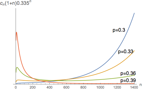
Recall that for the theoretical distribution of word lengths visited by the ERR random walk is
where is a normalizing constant. For the distribution cannot be normalised. In this case the function still contains information about the behaviour of the walk. If the random walk reaches a word of length then the relative heights of either side of describe the relative probabilities of increasing or decreasing the word length in the next move.
From Figure 4 we see that, for , the slope of is always positive, so at all word lengths probabilities are uniformly in favour of increasing the word length. However, as increases (and the growth rate for increases) a ‘hump’ appears at short word lengths. A random walk for such a group would tend to get stuck in the ‘hump’. Indeed, for the distribution looks much less like a walk diverging towards infinite word lengths and much more like the distributions for used to produce Figure 2, where the average word length in the ERR walk remained finite.
The distributions in Figure 4 exhibit a mechanism which can explain anomalous behaviour previously observed. When increases quickly the ERR random walk may adhere to the behaviour predicted by the theory and simultaneously give anomalous results about the asymptotics of the cogrowth function. In this sense if [9] contains incorrect answers it is because the original ERR algorithm as it was initially proposed asks the wrong question. The ERR walk does not measure asymptotic properties of the cogrowth function; it provides information about the cogrowth function only for word lengths visited by the walk. This observation forms the basis of Section 6.
Note that increasing the parameter pushes the algorithm towards longer word lengths. Thus, any pathological behaviour caused by the growth of could theoretically be overcome by increasing . If is known, then it may be used to calculate how large words have to get before divergence occurs. A method to do this is outlined by the following example.
Suppose that ERR random walks are run on a two generator group with (as in Figure 3). If we eliminate the term of the stationary distribution (which, being polynomial, becomes insignificant for long word lengths) the divergence properties are controlled by the contest between and . That is, divergence will occur when ; the word length at which divergence will occur is . If this value is known may be increased until the walk visits words of this length. This process, however, requires specific information about including all scaling constants. It is hard to imagine a group for which the sub-dominant cogrowth behaviour was known to this level of precision, but dominant cogrowth behaviour (and hence the amenability question for the group) was still unknown.
5.3. Reliability of the ERR results for Thompson’s group
In Proposition 3.11 we saw that the function for grows faster than that of any iterated wreath product of ’s, and certainly faster than that of any group. Since the ERR method fails to predict the amenability of these groups for as low as , and this behaviour is consistent with the pathological behaviour caused by , we conclude that the data encoded in Figure 1 does not imply the non-amenability of , and so the conclusion of the paper [9] that appears to be non-amenable based on this data is unreliable.
6. Appropriation of the ERR algorithm
The original implementation of the ERR random walk uses only the mean length of words visited in an attempt to estimate asymptotic behaviour of the cogrowth function. In this section we show that, using the full distribution of word lengths visited, it is possible to estimate specific values of the cogrowth function.
When doing a long random walk, the probability of arriving at a word of length can be estimated by multiplying the number of words of that length by the asymptotic probability that the walk ends at a word of this length, . That is,
The proportion of the time that the walks spends at words of length , however, gives us another estimate of . If we let be the number of times the walk visits a word of length then we have that
where is equal to the length of the walk. From this we obtain
For two different values, and , we obtain the result
Thus,
| (8) |
Equation 8 provides a method of estimating the value of using some known or previously estimated value of and the distribution of word lengths visited from an ERR random walk. Let’s try a quick implementation of this for Thompson’s group , where the first 48 cogrowth terms of which are known [17].
We ran an ERR random walk of length exceeding steps on the standard presentation (Equation 2) f or and . The frequency of word length visited is shown in Table 3.
We used Equation 8 and the data in Table 3 to estimate from , and then this estimate was used to estimate . (Note that the shortest non-empty trivial words are of length 10. Since the relators in the standard presentation of are even in length there are no odd length relators.) Using the data and the previous estimate for , estimates were made of the first 48 terms, and these compared to the correct value in Table 4.
This implementation of Equation 8 may be refined in several ways. Firstly, in many groups we have exact initial values of for more than the trivial result . In this case these initial values can be used to estimate subsequent terms. In this paper we are primarily concerned with testing the efficacy of this method for determining cogrowth, and so do not make use of such data.
Secondly, in the above implementation the only cogrowth value used to estimate was . Instead, estimates for may be made from for any . These estimates may then be averaged to form an estimate for . Note, however, that if only one ERR random walk is used, and each of the is itself estimated from previous values of the same distribution there may be issues with interdependence.
This leads naturally to the following refinement — to obtain several independent estimates for a given cogrowth value several ERR random walks can be run with different values for the parameters and .
6.1. The ERR-R algorithm.
The ERR-R algorithm accepts as input a group presentation and the cogrowth value with . As above, recursive application of Equation 8 is used to produce estimates for longer word lengths. However, in each step previous estimates for a range of are used to produce new estimates. A detailed analysis of the error incurred with each application of Equation 8 is performed in Section 6.5. All error bounds which appear in subsequent graphs are constructed using these techniques.
Unsurprisingly, the errror analysis in Section 6.5 predicts that the largest errors are incurred when data is used from the tails of random walk distributions. Ideally then, a separate random walk should be run for each , with parameters and chosen so that the sampled word lengths occupy the peaks of the distribution. If many estimates are to be made this is computationally infeasible. Instead we performed ERR random walks using a range of and values, which can be chosen so that all word lengths of interest are visited often.
When estimating , one estimate was made from each random walk distribution and from each . To avoid using the tails of distributions only data points which were greater than 10% of the max height were used.
Using Equation 9 each estimate was assigned a weight equal to the inverse of the estimated error. The final value for was taken as the weighted average of the estimates, and the error in was taken to be the weighted average of the individual error estimates.
Random walk data was obtained as before using the python code of the second author as described in Remark 4.2.
6.2. Application to the examples in Section 5
Applying the ERR-R algorithm can be used to analyse in more detail the pathological behaviours analysed in this paper. Unsurprisingly, for the presentations of the trivial group given in 5.1 which ignore the long relator, the ERR-R estimates for cogrowth values align closely with the three strand braid group. For we can use estimates of initial cogrowth to analyse how increases with . This is shown, for example in Figure 5 which exhibits the behaviour predicted by the convergence to in the space of marked groups. Further analysis of these presentations will appear in [27].

6.3. Application to surface group
The fundamental group of a surface of genus 2 has presentation . The cogrowth of this group has received a lot of attention, and good upper and lower bounds are known for the asymptotic rate of growth [14, 23].
ERR random walks were run on this surface group with and . Estimates were made for as well as the error . The resultant upper and lower bounds for are shown in Figure 6.

6.4. Application to Thompson’s group
We now apply the more sophisticated implementation of the method to . Recall that we can compare the first 48 values with exact values obtained by Haagerup et al.. Our method allows us to go much further than this though, which we do.
ERR random walks were run on with and . Collection of experimental data is ongoing. Table 5 shows comparisons between estimates for and the actual values, for , as well as the estimates for the error obtained from the experimental data.
Remark 6.1.
Table 5 shows a marked increase in the degree of accuracy of the estimates over those of Table 4. This suggests the method of using multiple distributions and weighted averages is effective. Note that there are approximately trivial words of length 48 so the walks could not possibly have visited each one. The sample of words visited by the walk seem to reflect the space as a whole reasonably accurately.
Figure 7 shows our estimates for upper and lower bounds of for .
6.5. Error analysis
Here we identify a method by which error in cogrowth estimates my be estimated. We stress that this is a statistical measurement of error, rather than theoretical.
Recall Equation 8. Suppose that is known up to , and that the error in the measurements and are and respectively. Then, from elementary calculus, the error in is given by
| (9) |
Hence the proportional error in the estimate of is approximately equal to the sum of the proportional errors in and . It is clear from this that if Equation 8 is used recursively (building new estimates based on previously estimated cogrowth values) the proportional error in is certain to increase. Note, the factor controlling the rate of growth in the proportional error of estimates is the proportional error in . If this is constant as increases the proportional error in will grow linearly with .
To calculate useful error margins for it is necessary to quantify . Here we employ the same method used in the ERR paper; walks are split into segments and the number of times the walk visits words of length is recorded for each segment. Let denote the number of times the walk visited words of length in the th segment. Then is taken to be the average of for and the error in is calculated from the statistical variance of these values,
| (10) |
6.6. Error in the -th root of
We have noted that recursive uses of Equation 8 will result in an increasing proportional error in . However, it is the -th root of which reflects the amenability of a group. Let and denote the error of the estimate for . Once again from elementary calculus we obtain that for a given
| (11) |
Thus, if increases at most linearly, can be expected to remain constant.
The values for grow exponentially, so a linearly increasing proportional error in corresponds with a massive increase in the absolute error in . In contrast, approaches a constant, so the proportional error depends linearly on the absolute error. Thus it is not surprising that our experimental results show that even when the error in cogrowth estimates grows large, the error in the -th root grows very slowly.
7. Conclusion
Several ideas emerge from this study. Firstly, researchers performing experimental mathematics to determine the amenability of a group need to take care that their algorithm is not susceptible to interference from sub-dominant behaviours. For the reduced-cogrowth function the sub-dominant behaviour is identified by . Amenability is an asymptotic property, and the interference of sub-dominant behaviours on experimental algorithms can be subtle and nuanced. In particular, we have shown that, if Thompson’s group is amenable, its function grows faster than any polynomial. This implies that the prediction of non-amenability of in [9] is unreliable.
We have also shown that, despite potential inaccuracies in estimates of asymptotics, the ERR-R method can produce accurate results for initial cogrowth values. These are interesting in their own right. Indeed, if Thompson’s group is not amenable, then its function need not be super-polynomial and results from experimental methods might well inform the construction of conjectures regarding cogrowth.
In this context the original benefits of the ERR algorithm still stand: it requires no group theoretic computational software, no solution to the word problem, and remains a computationally inexpensive way to quickly gain insight into the cogrowth function of a finitely presented group.
Acknowledgements
The authors wish to thank Andrew Rechnitzer and Andrew Elvey-Price for helpful feedback on this work.
References
- [1] G. N. Arzhantseva, V. S. Guba, M. Lustig, and J. Préaux. Testing Cayley graph densities. Ann. Math. Blaise Pascal, 15(2):233–286, 2008.
- [2] J. M. Belk and K. S. Brown. Forest diagrams for elements of Thompson’s group . Internat. J. Algebra Comput., 15(5-6):815–850, 2005.
- [3] A. Bendikov, C. Pittet, and R. Sauer. Spectral distribution and -isoperimetric profile of Laplace operators on groups. Math. Ann., 354(1):43–72, 2012.
- [4] M. G. Benli, R. I. Grigorchuk, and P. de la Harpe. Amenable groups without finitely presented amenable covers. Bull. Math. Sci., 3(1):73–131, 2013.
- [5] J. Burillo, S. Cleary, and B. Wiest. Computational explorations in Thompson’s group . In Geometric group theory, Trends Math., pages 21–35. Birkhäuser, Basel, 2007.
- [6] J. W. Cannon, W. J. Floyd, and W. R. Parry. Introductory notes on Richard Thompson’s groups. Enseign. Math. (2), 42(3-4):215–256, 1996.
- [7] T. G. Ceccherini-Silberstein and R. I. Grigorchuk. Amenability and growth of one-relator groups. Enseign. Math. (2), 43(3-4):337–354, 1997.
- [8] J. M. Cohen. Cogrowth and amenability of discrete groups. J. Funct. Anal., 48(3):301–309, 1982.
- [9] M. Elder, A. Rechnitzer, and E. J. Janse van Rensburg. Random sampling of trivial words in finitely presented groups. Exp. Math., 24(4):391–409, 2015.
- [10] M. Elder, A. Rechnitzer, and T. Wong. On the cogrowth of Thompson’s group . Groups Complex. Cryptol., 4(2):301–320, 2012.
- [11] A. Erschler. On isoperimetric profiles of finitely generated groups. Geom. Dedicata, 100:157–171, 2003.
- [12] P. Flajolet and R. Sedgewick. Analytic Combinatorics. Cambridge University Press, 2009.
- [13] E. Følner. On groups with full Banach mean value. Math. Scand., 3:243–254, 1955.
- [14] S. Gouëzel. A numerical lower bound for the spectral radius of random walks on surface groups. Combin. Probab. Comput., 24(6):838–856, 2015.
- [15] R. I. Grigorchuk. Symmetrical random walks on discrete groups. In Multicomponent random systems, volume 6 of Adv. Probab. Related Topics, pages 285–325. Dekker, New York, 1980.
- [16] V. S. Guba and M. V. Sapir. On subgroups of the R. Thompson group and other diagram groups. Mat. Sb., 190(8):3–60, 1999.
- [17] S. Haagerup, U. Haagerup, and M. Ramirez-Solano. A computational approach to the Thompson group . Internat. J. Algebra Comput., 25(3):381–432, 2015.
- [18] H. Kesten. Symmetric random walks on groups. Trans. Amer. Math. Soc., 92:336–354, 1959.
- [19] D. Kouksov. On rationality of the cogrowth series. Proc. Amer. Math. Soc., 126(10):2845–2847, 1998.
- [20] P. H. Kropholler and A. Martino. Graph-wreath products and finiteness conditions. J. Pure Appl. Algebra, 220(1):422–434, 2016.
- [21] D. Kuksov. Cogrowth series of free products of finite and free groups. Glasg. Math. J., 41(1):19–31, 1999.
- [22] J. T. Moore. Fast growth in the Følner function for Thompson’s group . Groups Geom. Dyn., 7(3):633–651, 2013.
- [23] T. Nagnibeda. An upper bound for the spectral radius of a random walk on surface groups. Zap. Nauchn. Sem. S.-Peterburg. Otdel. Mat. Inst. Steklov. (POMI), 240(Teor. Predst. Din. Sist. Komb. i Algoritm. Metody. 2):154–165, 293–294, 1997.
- [24] C. Pittet and L. Saloff-Coste. On the stability of the behavior of random walks on groups. J. Geom. Anal., 10(4):713–737, 2000.
- [25] C. Pittet and L. Saloff-Coste. On random walks on wreath products. Ann. Probab., 30(2):948–977, 2002.
- [26] C. Pittet and L. Saloff-Coste. Random walks on finite rank solvable groups. J. Eur. Math. Soc. (JEMS), 5(4):313–342, 2003.
- [27] C. Rogers. On the interconnectedness, via random walks, of cogrowth rates and the Følner function. PhD thesis, The University of Newcastle, 2016.
- [28] R. Szwarc. A short proof of the Grigorchuk-Cohen cogrowth theorem. Proc. Amer. Math. Soc., 106(3):663–665, 1989.
- [29] A. M. Vershik. Amenability and approximation of infinite groups. Selecta Math. Soviet., 2(4):311–330, 1982. Selected translations.
- [30] W. Woess. Cogrowth of groups and simple random walks. Arch. Math. (Basel), 41(4):363–370, 1983.