跳到论文正文
W Papers独立论文阅读器 arXiv:1608.06637 论文正文 计算阅读时间 · 0%
引用这篇论文根据当前论文元数据生成,正式投稿前建议核对。


License: arXiv.org perpetual non-exclusive license
arXiv:1608.06637v1 [cond-mat.str-el] 23 Aug 2016

Realizing infrared power-law liquids in the cuprates from unparticle interactions

Kridsanaphong Limtragool, Chandan Setty, Zhidong Leong, and Philip W. Phillips Affiliation: Department of Physics and Institute for Condensed Matter Theory, University of Illinois 1110 W. Green Street, Urbana, IL 61801, U.S.A.
August 24, 2026
Abstract

Recent photoemission experiments [1] reveal that the excitations along the nodal region in the strange metal of the cuprates, rather than corresponding to poles in the single-particle Green function, exhibit power-law scaling as a function of frequency and temperature. Because such power-law scaling is indicative of a scale-invariant sector, as a first step, we perturbatively evaluate the electron self-energy due to interactions with scale-invariant unparticles. We focus on a G0​WG_{0}W type diagram with an interaction WW mediated by a bosonic scalar unparticle. We find that, in the high-temperature limit, the imaginary part of the self-energy Im​Σ\mathrm{Im}\Sigma is linear in temperature. In the low-temperature limit, Im​Σ\mathrm{Im}\Sigma exhibits the same power law in both temperature and frequency, with an exponent that depends on the scaling dimension of an unparticle operator. Such behavior is qualitatively consistent with the experimental observations. We then expand the unparticle propagator into coherent and incoherent contributions, and study how the incoherent part violates the density of states (DOS) and density-density correlation function sum rules (f-sum rule). Such violations can, in principle, be observed experimentally. Our work indicates that the physical mechanism for the origin of the power-law scaling is the incoherent background, which is generated from the Mott-scale physics.

I Introduction

Scale invariance is the cornerstone of any infrared theory or physical system in which the physics is controlled by a critical fixed point. It is surprising then that recent photoemission experiments [1] on the strange metal phase of the cuprates indicate that scale invariance is applicable not just at a single (quantum critical) point, but over an entire phase. The experiments reveal that the excitations along the nodal direction are not at all quasiparticle-like, but rather exhibit a power-law scaling in which frequency and temperature are interchangeable. Specifically, they find [1] that the scattering rates inferred from the momentum distribution curves (MDCs) along the nodal direction exhibit a power-law scaling of the form,

ΣPLL​(ω)=Γ0+λ​((ℏ​ω)2+(γ​kB​T)2)a(ℏ​ωN)2​a−1,\displaystyle\Sigma_{\rm PLL}(\omega)=\Gamma_{0}+\lambda\frac{((\hbar\omega)^{2}+(\gamma k_{B}T)^{2})^{a}}{(\hbar\omega_{N})^{2a-1}}, (1)

where ωN\omega_{N} is a normalization energy scale, and γ\gamma and λ\lambda are constants. This scaling form of the self-energy, motivated by that of marginal Fermi liquid theory [2] and Anderson’s [3] “Hidden Fermi Liquid”, is found to hold over a wide range of dopings — from underdoped where a<1/2a<1/2, to optimal doping where a=1/2a=1/2, and to overdoped with a>1/2a>1/2. While scaling has been observed previously, it was typically associated with just a single doping level, namely at the optimal concentration [4, 5, 6].

It is the modeling and possible origin of such power-law scaling over an entire phase that we address here. Scale invariance over a wide range does have some precedence, at least theoretically. For example, the spectral functions calculated within the AdS/CFT formalism exhibit a range of power law scaling as the scaling dimension of the boundary fermionic operator is tuned continuously [7, 8]. Building on this set of ideas, one of us [9] proposed that the strange metal is described by a scale-invariant sector over the entire range of doping. The key computational tool used here is the unparticle propagators proposed by Georgi [10]. The unparticle propagators were modeled within the continuous mass formalism. If ϕ⁡(p,m2)\phi(p,m^{2}) is a scalar propagator with four momentum p and mass squared m2m^{2}, the propagator for the unparticle (Gu​(p)G_{u}(p)) can be obtained as [11, 12] Gu​(p)=∫0∞d​m2​ϕ​(p,m2)​f2​(m2)G_{u}(p)=\int_{0}^{\infty}dm^{2}\phi(p,m^{2})f^{2}(m^{2}) with ϕ⁡(p,m2)=1p2−m2+i​η\phi(p,m^{2})=\frac{1}{p^{2}-m^{2}+i\eta}. The function f⁡(m2)f(m^{2}) is a weighing function such that the number of fields between m2m^{2} and m2+d​m2m^{2}+dm^{2} is f⁡(m2)​d​m2f(m^{2})dm^{2}. If we choose f⁡(m2)=(m2)(du−d+12)/2f(m^{2})=(m^{2})^{(d_{u}-\frac{d+1}{2})/2} where d+1d+1 is the spacetime dimension and dud_{u} is the scaling dimension of the unparticle operator, we obtain the unparticle propagator

Gu​(p)∼1(−p2−i​η)d+12−du.G_{u}(p)\sim\frac{1}{(-p^{2}-i\eta)^{\frac{d+1}{2}-d_{u}}}. (2)

Alternatively, to construct unparticles, one can start from the action of a massive scalar field [9] and integrate over the mass m2m^{2} (again assuming a mass distribution) by treating it as an additional coordinate so that scale invariance is restored. The new action can then be rewritten into a theory in the anti-de Sitter space-time (AdS). The resulting two point function obtained from the AdS/CFT correspondence can be identified as the unparticle propagator. It is clear from the form of the unparticle propagator that the exponent d+12−du\frac{d+1}{2}-d_{u} is, in general, not an integer. This yields branch points at ±k2\pm\textbf{k}^{2} (instead of poles), indicating that unparticles represent incoherent electronic states of matter that lack a “particle-like” character, and are associated with measurable quantities that encompass the physics from both low and high energy scales.

A question that remains open from this work is how the unparticle sector interact with the particle sector to renormalize the quasiparticle weights. Physically, the unparticle sector should be thought of as the incoherent part of the spectrum. The question we address here is: what is the fate of particles in the presence of an incoherent sector? This question is of utmost relevance at present since the experiments indicate that it is the electron scattering rate that exhibits a power-law scaling. Ultimately, a secondary question that rises is what role do unparticle-unparticle interactions play. We postpone the latter question to a subsequent paper and focus here on the former to see how close we can come to a description of the power-law liquid with just electron-unparticle interactions. Consequently, to address the experiments, we consider the interaction between electrons and the unparticle sector directly. The quantity we focus on is a quasiparticle’s lifetime τ\tau, which is proportional to the imaginary part of electron’s self-energy. In particular, we want to know how τ\tau depends on the temperature, TT, and frequency, ω\omega, and in what situation τ\tau exhibits a power law as a result of interactions with the scale-invariant sector. We evaluate electron self-energies perturbatively using a G0​WG_{0}W type diagram in which the interaction WW is mediated by the bosonic scalar unparticle sector. We find that at high temperatures, the quasiparticle’s lifetime is linear in TT as a result of bosonic excitations of unparticles. In the low-temperature limit, the electron’s energy dispersion becomes linear in momentum and thus the scaling analysis can be applied. The quasiparticle’s lifetime in this case is a power law of the form τ∼Td−2+2​α\tau\sim T^{d-2+2\alpha} and τ∼|ω|d−2+2​α\tau\sim|\omega|^{d-2+2\alpha}, where 1−α=d+12−du1-\alpha=\frac{d+1}{2}-d_{u}. To satisfy the unitarity bound[13] du>(d−1)/2d_{u}>(d-1)/2, the only constraint on α\alpha is α>0\alpha>0. However, in perturbation theory, further constraints arising from the Matsubara summations and the convergence of the integrals place α\alpha in the interval (3−d)/2<α<1(3-d)/2<\alpha<1. Hence, while the current perturbative particle-unparticle treatment can describe non-trivial power-law behaviour of the self-energy with respect to temperature and frequency, it cannot access the regime α<(3−d)/2\alpha<(3-d)/2 where the current theory gives infrared divergences. Whether the divergences which arise for α<(3−d)/2\alpha<(3-d)/2 vanish when unparticle-unparticle interactions are included will be explored in a further publication. We then turn our attention to a problem regarding a violation of a sum rule when unparticles are present in a system. In this discussion, instead of using the bosonic unparticles, we use a fermionic propagator with a fractional power, since the results obtained can be readily compared with known standard sum rules. We expand the propagator into coherent and incoherent contributions, and study how the incoherent part violates the density of states (DOS) and density-density correlation function sum rules.

II Electron-Unparticle

We investigate a system consisting of electrons that interact with a scale invariant sector. We model such a scale invariant sector by a bosonic scalar unparticle with a momentum cutoff Λ\Lambda. The cutoff signifies that the unparticle is an effective infrared description of some high energy model. The interaction between an electron and an unparticle is chosen to be a constant Yukawa coupling, uu. The action of the model we consider in Matsubara-Fourier space is given by

S\displaystyle S =\displaystyle= T​∑m∫Λdd​p(2​π)d​ϕm​(𝐩)​Gu,m−1​(𝐩)​ϕm​(𝐩)\displaystyle T\sum\limits_{m}\int\limits^{\Lambda}\frac{d^{d}p}{(2\pi)^{d}}\phi_{m}({\mathbf{p}})G^{-1}_{u,m}({\mathbf{p}})\phi_{m}({\mathbf{p}})
−T∑n∫dd​q(2​π)dψn†(𝐪)Ge,n−1(𝐪)ψn(𝐪)\displaystyle-T\sum\limits_{n}\int\limits\frac{d^{d}q}{(2\pi)^{d}}\psi^{\dagger}_{n}({\mathbf{q}})G^{-1}_{e,n}({\mathbf{q}})\psi_{n}({\mathbf{q}})
+uT2∑m,n∫Λdd​p(2​π)d∫dd​q(2​π)dψm+n†(𝐩+𝐪)ϕm(𝐩)ψn(𝐪)\displaystyle+uT^{2}\sum\limits_{m,n}\int\limits^{\Lambda}\frac{d^{d}p}{(2\pi)^{d}}\int\limits\frac{d^{d}q}{(2\pi)^{d}}\psi^{\dagger}_{m+n}({\mathbf{p}}+{\mathbf{q}})\phi_{m}({\mathbf{p}})\psi_{n}({\mathbf{q}})

where ϕ\phi is a bosonic unparticle and ψ\psi is a non-relativistic electron field. Here, GuG_{u} is the unparticle propagator, GeG_{e} is the non-interacting electron propagator, TT denotes the temperature, and the subscripts of the fields and the propagators denote the dependence on Matsubara frequency. The bosonic unparticle propagator is given by

Gu,m​(𝐩)=1(ωm2+E𝐩2)1−α,\displaystyle G_{u,m}({\mathbf{p}})=\frac{1}{(\omega_{m}^{2}+E^{2}_{{\mathbf{p}}})^{1-\alpha}}, (4)

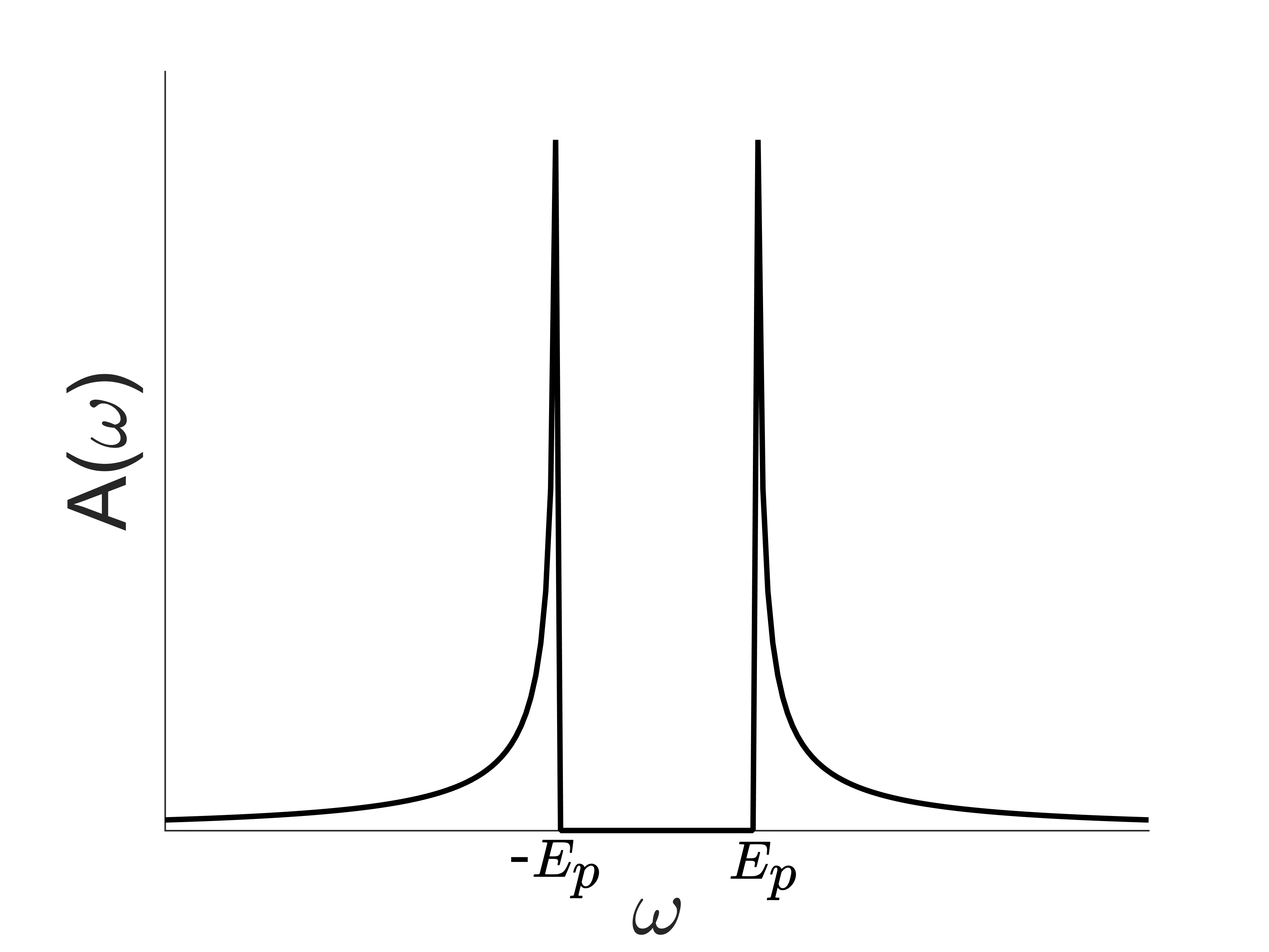
where α\alpha is related to dd and dud_{u} by 1−α=d+12−du1-\alpha=\frac{d+1}{2}-d_{u}, and E𝐩E_{{\mathbf{p}}} is a quantity with units of energy. Since the spectral function calculated from GuG_{u} is gapped between −E𝐩-E_{{\mathbf{p}}} and E𝐩E_{{\mathbf{p}}} (Fig. 1), E𝐩E_{{\mathbf{p}}} can be interpreted as the minimum energy required to excite an unparticle of momentum pp.

Refer to caption
Figure 1: The spectral function of unparticles when 0<α<10<\alpha<1.

We choose E𝐩E_{{\mathbf{p}}} to have a form E𝐩=|𝐩|​v=p​vE_{{\mathbf{p}}}=|{\mathbf{p}}|v=pv in order for GuG_{u} to be scale covariant. Here, vv is a dimensionless constant. If α=0\alpha=0, GuG_{u} turns into a propagator of a free scalar field. The electron propagator GeG_{e} is given by

Ge,n​(𝐪)=1i​ωn−ε𝐪,\displaystyle G_{e,n}({\mathbf{q}})=\frac{1}{i\omega_{n}-\varepsilon_{{\mathbf{q}}}}, (5)

where ε𝐩=p22​m−μ\varepsilon_{{\mathbf{p}}}=\frac{{p}^{2}}{2m}-\mu and μ=εf\mu=\varepsilon_{f} is the chemical potential which we assume to be temperature independent.

We want to point out that the system of electrons and unparticles we consider here resembles the standard electron-phonon system modeled by the Fröhlich Hamiltonian [14], but with key differences. In contrast to the phonon being a quanta of lattice vibration, the unparticle in our model is an effective scale invariant object of some high energy model, such as the Mott physics in the Hubbard model. It is the lack of the quanta concept being relevant to unpartices that is the origin of the branch-cut behavior of the unparticle propagator. Nonetheless, as with phonons, unparticle stuff exists only up to Λ\Lambda in the same way that phonon has a momentum cutoff ∼1/a\sim 1/a with aa being a lattice spacing.

Refer to caption
Figure 2: The Feynman diagram for the electron’s self-energy. The solid line represents an electron propagator. The dashed line represents an unparticle propagator.

We are interested in the quasiparticle’s lifetime τ\tau which is given by τ=−12​Im​Σ\tau=-\frac{1}{2}\mathrm{Im}\Sigma, where Σ\Sigma is the electron’s self-energy. The expression for the electron self-energy at the lowest order (Fig. 2) as a function of fermionic Matsubara frequency ωn\omega_{n} and momentum qq can be written as

Σn​(𝐪)\displaystyle\Sigma_{n}({\mathbf{q}}) =\displaystyle= u2​∫dd​p(2​π)d​T​∑mGu,m​(𝐩)​Ge,n+m​(𝐪+𝐩).\displaystyle u^{2}\int\frac{d^{d}p}{(2\pi)^{d}}T\sum\limits_{m}G_{u,m}({\mathbf{p}})G_{e,n+m}({\mathbf{q}}+{\mathbf{p}}). (6)

We perform the summation over the bosonic Matsubara frequency ωm\omega_{m} using the standard contour integral technique (see Appendix A). We then perform an analytic continuation, i​ωn→ω+i​ηi\omega_{n}\rightarrow\omega+i\eta, to obtain the retarded self-energy. The self-energy in the case of 0<α<10<\alpha<1 is

Σ⁡(ω,𝐪)\displaystyle\Sigma(\omega,{\mathbf{q}}) =\displaystyle= −u2∫dd​p(2​π)dgF​(ε𝐩+𝐪)(−ε𝐩+𝐪+E𝐩+ω+i​η)1−α​(ε𝐩+𝐪+E𝐩−ω−i​η)1−α\displaystyle-u^{2}\int\frac{d^{d}p}{(2\pi)^{d}}\frac{g_{F}(\varepsilon_{{\mathbf{p}}+{\mathbf{q}}})}{(-\varepsilon_{{\mathbf{p}}+{\mathbf{q}}}+E_{{\mathbf{p}}}+\omega+i\eta)^{1-\alpha}(\varepsilon_{{\mathbf{p}}+{\mathbf{q}}}+E_{{\mathbf{p}}}-\omega-i\eta)^{1-\alpha}} (7)
+sin⁡(π​α)πu2∫dd​p(2​π)d∫E𝐩∞dzgB​(z)(z+E𝐩)1−α​(z−E𝐩)1−α(1(z+ω+i​η−ε𝐩+𝐪)−1(z−ω−i​η+ε𝐩+𝐪)),\displaystyle+\frac{\sin(\pi\alpha)}{\pi}u^{2}\int\frac{d^{d}p}{(2\pi)^{d}}\int\limits_{E_{{\mathbf{p}}}}^{\infty}dz\frac{g_{B}(z)}{(z+E_{{\mathbf{p}}})^{1-\alpha}(z-E_{{\mathbf{p}}})^{1-\alpha}}\bigg(\frac{1}{(z+\omega+i\eta-\varepsilon_{{\mathbf{p}}+{\mathbf{q}}})}-\frac{1}{(z-\omega-i\eta+\varepsilon_{{\mathbf{p}}+{\mathbf{q}}})}\bigg),

where gF​(z)=12​tanh⁡(β​z2)g_{F}(z)=\frac{1}{2}\tanh(\frac{\beta z}{2}) is a fermionic factor and gB​(z)=12​coth⁡(β​z2)g_{B}(z)=\frac{1}{2}\coth(\frac{\beta z}{2}) is a bosonic factor obtained from converting the summation to the contour integral. Here, the phase angle needed when one evaluates the power 1−α1-\alpha in the first term is in the range −π≤θ<π-\pi\leq\theta<\pi. We denote the first term by ΣF\Sigma_{F} and the second term by ΣB\Sigma_{B} since their integrands contain the fermionic and bosonic factors. We are interested in the behavior of the imaginary part of this self-energy as a function of temperature and frequency.

II.1 Behavior of Im​Σ​(T)\mathrm{Im}\Sigma(T)

We now turn to the evaluation of the relevant terms. When T≫|ε𝐩+𝐪|T\gg|\varepsilon_{{\mathbf{p}}+{\mathbf{q}}}|, we have gF​(ε𝐩+𝐪)=12​tanh⁡β​ε𝐩+𝐪2≈β​ϵ𝐩+𝐪4g_{F}(\varepsilon_{{\mathbf{p}}+{\mathbf{q}}})=\frac{1}{2}\tanh\frac{\beta\varepsilon_{{\mathbf{p}}+{\mathbf{q}}}}{2}\approx\frac{\beta\epsilon_{{\mathbf{p}}+{\mathbf{q}}}}{4}. Hence, the first term in Eq. 7, ΣF\Sigma_{F}, goes like O⁡(1T)O(\frac{1}{T}). Taking the imaginary part of the second term in Eq. 7 and then integrating over zz using the delta functions, one obtains

Im​ΣB​(ω,𝐪)\displaystyle\mathrm{Im}\ \Sigma_{B}(\omega,{\mathbf{q}}) =\displaystyle= −sin(πα)u2∫dd​p(2​π)d(Θ(−ω+ε𝐩+𝐪−E𝐩)gB​(−ω+ε𝐩+𝐪)(−ω+ε𝐩+𝐪+E𝐩)α​(−ω+ε𝐩+𝐪−E𝐩)α\displaystyle-\sin(\pi\alpha)u^{2}\int\frac{d^{d}p}{(2\pi)^{d}}\Bigg(\Theta(-\omega+\varepsilon_{{\mathbf{p}}+{\mathbf{q}}}-E_{{\mathbf{p}}})\frac{g_{B}(-\omega+\varepsilon_{{\mathbf{p}}+{\mathbf{q}}})}{(-\omega+\varepsilon_{{\mathbf{p}}+{\mathbf{q}}}+E_{{\mathbf{p}}})^{\alpha}(-\omega+\varepsilon_{{\mathbf{p}}+{\mathbf{q}}}-E_{{\mathbf{p}}})^{\alpha}} (8)
OPEN+Θ⁡(ω−ε𝐩+𝐪−E𝐩)​gB​(ω−ε𝐩+𝐪)(ω−ε𝐩+𝐪+E𝐩)α​(ω−ε𝐩+𝐪−E𝐩)α).\displaystyle\hskip 68.99895pt+\Theta(\omega-\varepsilon_{{\mathbf{p}}+{\mathbf{q}}}-E_{{\mathbf{p}}})\frac{g_{B}(\omega-\varepsilon_{{\mathbf{p}}+{\mathbf{q}}})}{(\omega-\varepsilon_{{\mathbf{p}}+{\mathbf{q}}}+E_{{\mathbf{p}}})^{\alpha}(\omega-\varepsilon_{{\mathbf{p}}+{\mathbf{q}}}-E_{{\mathbf{p}}})^{\alpha}}\Bigg).

In the high-temperature limit, gB​(z)g_{B}(z) can be expanded as gB​(z)=12​tanh⁡β​z2→1β​z+O⁡(β​z).g_{B}(z)=\frac{1}{2}\tanh\frac{\beta z}{2}\rightarrow\frac{1}{\beta z}+O(\beta z). So when T≫|ϵ𝐩+𝐪−ω|T\gg|\epsilon_{{\mathbf{p}}+{\mathbf{q}}}-\omega|, Im​ΣB​(ω,𝐪)=−C​u2​T+O⁡(1T)\mathrm{Im}\Sigma_{B}(\omega,{\mathbf{q}})=-Cu^{2}T+O(\frac{1}{T}) where CC is a temperature-independent constant. Consequently, in the high-temperature limit, one has

Im​Σ=Im​ΣF+Im​ΣB∝−T.\displaystyle\mathrm{Im}\Sigma=\mathrm{Im}\Sigma_{F}+\mathrm{Im}\Sigma_{B}\propto-T. (9)

Since we do not explicitly use the form E𝐩=p​vE_{{\mathbf{p}}}=pv in the above argument, this result also holds for any form of E𝐩E_{{\mathbf{p}}}, provided the integral in Eq. 8 converges.

For the low-temperature case, we consider only the electrons on the Fermi surface (𝐪=𝐪f{\mathbf{q}}={\mathbf{q}}_{f}) with ω=0\omega=0. In this case, the expression ε𝐩+𝐪\varepsilon_{{\mathbf{p}}+{\mathbf{q}}} simplifies to ε𝐩+𝐪=p22​m+𝐩⋅𝐪m\varepsilon_{{\mathbf{p}}+{\mathbf{q}}}=\frac{{p}^{2}}{2m}+\frac{{\mathbf{p}}\cdot{\mathbf{q}}}{m}. If the momentum cutoff Λ\Lambda is much smaller than qfq_{f}, it should be reasonable to omit the term p22​m\frac{{p}^{2}}{2m} in ε𝐩+𝐪\varepsilon_{{\mathbf{p}}+{\mathbf{q}}}. From Eq. 7, we separate the temperature dependent parts using gF​(z)=12−nF​(z)g_{F}(z)=\frac{1}{2}-n_{F}(z) and gB​(z)=12+nB​(z)g_{B}(z)=\frac{1}{2}+n_{B}(z) where nFn_{F} and nBn_{B} are the Fermi and Bose distributions, respectively. We drop the 12\frac{1}{2} terms from gFg_{F} and gBg_{B}, since we are only interested in the temperature dependence of Σ\Sigma. Performing the change of variables z→p​z′z\rightarrow pz^{\prime} and p→p​Tp\rightarrow pT, one obtains

Σ\displaystyle\Sigma =\displaystyle= u2​Td−2+2​α​∫Λ/Tdd​p(2​π)d​p−2+2​α​1(ep⋅𝐪fm+1)​(−p^⋅𝐪fm+v+i​η)1−α​(p^⋅𝐪fm+v−i​η)1−α\displaystyle u^{2}T^{d-2+2\alpha}\int\limits^{\Lambda/T}\frac{d^{d}p}{(2\pi)^{d}}p^{-2+2\alpha}\frac{1}{(e^{\frac{p\cdot{\mathbf{q}}_{f}}{m}}+1)(-\frac{\hat{p}\cdot{\mathbf{q}}_{f}}{m}+v+i\eta)^{1-\alpha}(\frac{\hat{p}\cdot{\mathbf{q}}_{f}}{m}+v-i\eta)^{1-\alpha}}
+sin⁡(π​α)πu2Td−2+2​α∫Λ/Tdd​p(2​π)dp−2+2​α∫v∞dz′1(ep​z′−1)​(z′+v)1−α​(z′−v)1−α(1(z′+i​η−p^⋅𝐪fm)−1(z′−i​η+p^⋅𝐪fm))\displaystyle+\frac{\sin(\pi\alpha)}{\pi}u^{2}T^{d-2+2\alpha}\int\limits^{\Lambda/T}\frac{d^{d}p}{(2\pi)^{d}}p^{-2+2\alpha}\int\limits_{v}^{\infty}dz^{\prime}\frac{1}{(e^{pz^{\prime}}-1)(z^{\prime}+v)^{1-\alpha}(z^{\prime}-v)^{1-\alpha}}\bigg(\frac{1}{(z^{\prime}+i\eta-\frac{\hat{p}\cdot{\mathbf{q}}_{f}}{m})}-\frac{1}{(z^{\prime}-i\eta+\frac{\hat{p}\cdot{\mathbf{q}}_{f}}{m})}\bigg)

where p^\hat{p} denotes a unit vector in the direction of 𝐩{\mathbf{p}}. Upon taking the limit T→0T\rightarrow 0, the upper limit of the momentum integral can be taken to ∞\infty provided that there is no infrared divergence from the integrals over pp. By counting the powers of pp, one needs d−3+2​α>0d-3+2\alpha>0, i.e. α>0\alpha>0 for d=3d=3 and α>0.5\alpha>0.5 for d=2d=2. Therefore, one has

Im​Σ∝−Td−2+2​α\displaystyle\mathrm{Im}\Sigma\propto-T^{d-2+2\alpha} (11)

at low temperatures. If the coupling constant uu depends on momentum 𝐩{\mathbf{p}}, the criterion for the absence of the infrared divergence and the scaling of Im​Σ\mathrm{Im}\Sigma will be different. A more in-depth analysis for the d=3d=3 case in Appendix B shows that when Λ2<qf−m​v\frac{\Lambda}{2}<q_{f}-mv and m​v<qfmv<q_{f} the term p22​m\frac{p^{2}}{2m} in ε𝐩+𝐪\varepsilon_{{\mathbf{p}}+{\mathbf{q}}} contributes to Im​Σ\mathrm{Im}\Sigma as O⁡(Td−1+2​α)O(T^{d-1+2\alpha}). This results justifies our omission of the p22​m\frac{p^{2}}{2m} term in the scaling analysis above. The same argument used in Appendix B cannot be applied to the d=2d=2 case. Nevertheless, the numerical results below indicate that Eq. 11 still holds for the case d=2d=2 and α>0.5\alpha>0.5 (see Fig. 4).

Refer to caption
(a) d=3d=3 and α=0.8\alpha=0.8
Refer to caption
(b) d=2d=2 and α=0.8\alpha=0.8
Figure 3: Log-log plots of the imaginary part of the self-energy as a function of temperature.
Refer to caption
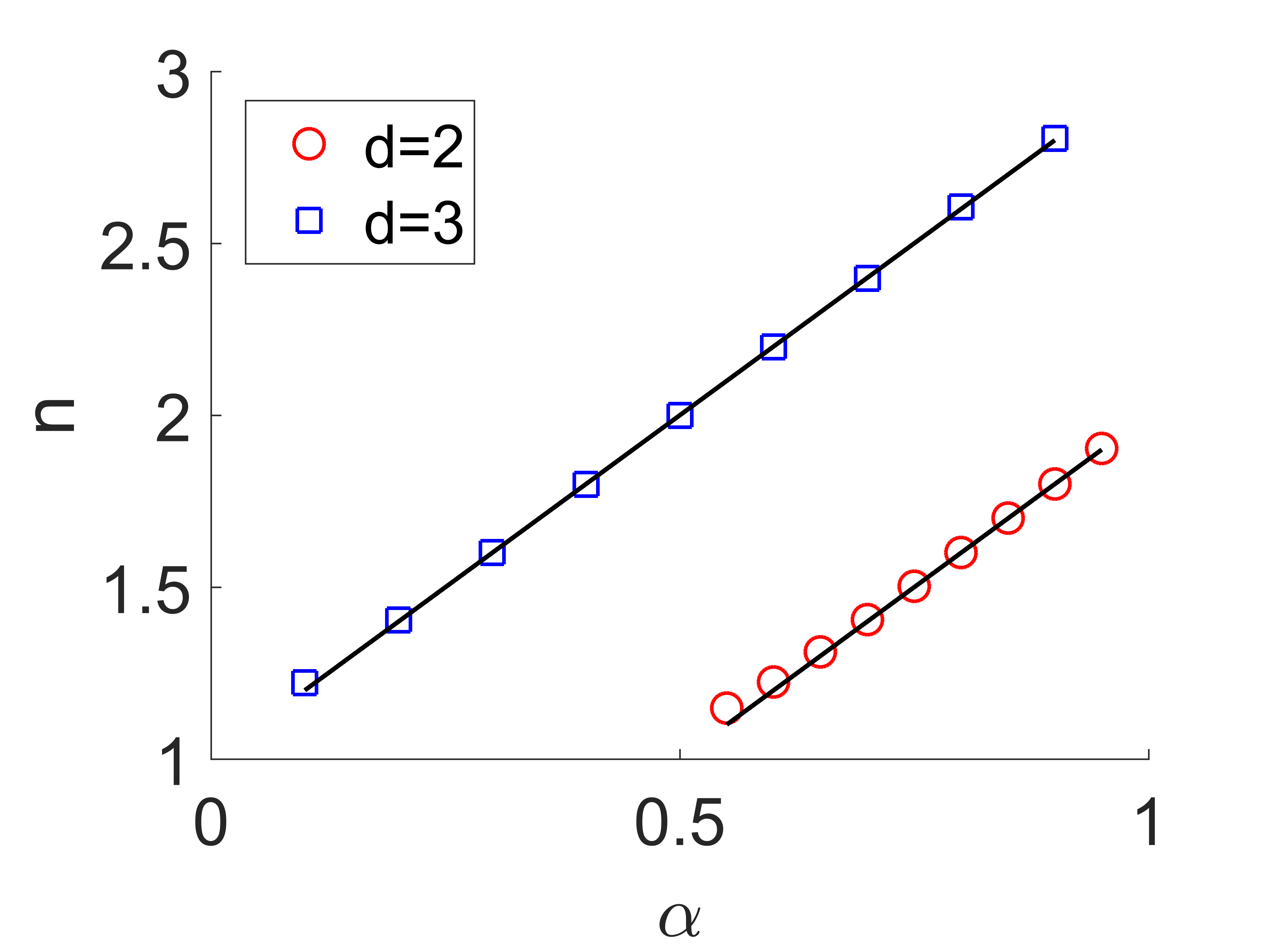
Figure 4: Plots of Im​Σ\mathrm{Im}\Sigma’s temperature power law exponent nn vs. α\alpha at low temperatures. Squares and circles correspond to the exponents obtained by fitting the low TT parts of Im​Σ\mathrm{Im}\Sigma to power law in d=3d=3 and d=2d=2, respectively. Black lines are the plots of n=d−2+2​αn=d-2+2\alpha.

We numerically evaluate the imaginary part of the self-energy as a function of temperature using Eq. 42 for d=3d=3 and Eq. 51 for d=2d=2. Here we use Λ=m\Lambda=m, qf=2​mq_{f}=\sqrt{2}m, and v=0.4v=0.4. With these parameters, the conditions Λ2<qf−m​v\frac{\Lambda}{2}<q_{f}-mv and m​v<qfmv<q_{f} are satisfied. The results for the α=0.8\alpha=0.8 case are shown in Figs. 3(a) and 3(b). We find that, for both the d=3d=3 and d=2d=2 cases, Im​Σ\mathrm{Im}\Sigma depends linearly on temperature at large TT. At low TT, Im​Σ\mathrm{Im}\Sigma exhibits a power law ∼Tn\sim T^{n}. The exponent nn follows Eq. 11 for d=3d=3 when 0<α<10<\alpha<1, and for d=2d=2 when 0.5<α<10.5<\alpha<1 as shown in Fig. 4.

II.2 Behavior of Im​Σ​(ω)\mathrm{Im}\Sigma(\omega)

Refer to caption
(a) Low temparture T=0.01​mT=0.01m
Refer to caption
(b) High temperature T=mT=m
Figure 5: Plots of the imaginary part of the self-energy as a function of frequency in the case α=0.7\alpha=0.7 and d=3d=3.
Refer to caption
Figure 6: Plot of Im​Σ\mathrm{Im}\Sigma’s frequency power law exponent nn vs. α\alpha at low frequency and temperature (T=0.01​mT=0.01m). The spatial dimension in this case is d=3d=3. Squares (Circles) correspond to exponents obtained by fitting the positive (negative) ω\omega part of Im​Σ\mathrm{Im}\Sigma to a power law. The black line is the plot of n=d−2+2​αn=d-2+2\alpha.

We numerically study Im​Σ​(ω)\mathrm{Im}\Sigma(\omega) using the sum of Eq. 34 and the imaginary part of Eq. 26. The term Σϵ\Sigma_{\epsilon} (Appendix A.3) is now included because the integral over zz in Eq. 34 needs a finite lower limit, ϵ\epsilon. We work in d=3d=3 and use the same parameters as in Sect. II.1, i.e. Λ=m\Lambda=m, q=qf=2​mq=q_{f}=\sqrt{2}m, and v=0.4v=0.4. The results are displayed in Fig. 5(a) for the low-temperature case, and in Fig. 5(b) for the high-temperature case. We find that, in the low-temperature case, Im​Σ​(ω)\mathrm{Im}\Sigma(\omega) exhibits a power law at low frequencies. This power law has the form

Im​Σ∼|ω|d−2+2​α\displaystyle\mathrm{Im}\Sigma\sim|\omega|^{d-2+2\alpha} (12)

as shown in Fig. 6.

II.3 Discussion

We found that, at high temperatures, the imaginary part of the electron’s self-energy depends linearly on temperature. The linear TT behavior is a common feature in a system of fermions interacting with bosons. One well-known example is an electron-phonon system in metals [14]. In the context of unparticles, this result is somewhat of a surprise as there is no concept of quantization. Mathematically, the origin of the TT-linear behavior seems to arise from the summation over the bosonic Matsubara frequency in a self-energy diagram (Fig. 2) which yields the Bose factor gB=12​coth⁡(ε2​T)g_{B}=\frac{1}{2}\coth(\frac{\varepsilon}{2T}). Since the leading term in the large TT expansion of gBg_{B} is proportional of TT, the imaginary part of the self-energy is also linear in TT.

At low temperatures, Im​Σ\mathrm{Im}\Sigma of the electron on the Fermi surface exhibits a fractional power law of the form Td−2+2​αT^{d-2+2\alpha} and |ω|d−2+2​α|\omega|^{d-2+2\alpha}, in qualitative agreement with the experiments [1]. This power law behavior occurs because the excitation energy of electrons close to the Fermi surface becomes linear in momentum i.e. ε𝐩+𝐪f∝p\varepsilon_{{\mathbf{p}}+{\mathbf{q}}_{f}}\propto p. One can see this by noting that when the momentum cutoff Λ\Lambda of the unparticles is much smaller than the Fermi momentum, it is reasonable to drop the p2/2​m{p}^{2}/2m term in ε𝐩+𝐪f\varepsilon_{{\mathbf{p}}+{\mathbf{q}}_{f}}. For the d=3d=3 case, we give a precise argument that justifies the omission of the p2{p}^{2} term in Appendix B. The scaling obtained for Im​Σ\mathrm{Im}\Sigma by using ε𝐩+𝐪f∝p\varepsilon_{{\mathbf{p}}+{\mathbf{q}}_{f}}\propto p is ∝T1+2​α\propto T^{1+2\alpha} and the error from neglecting the p2p^{2} term in ε𝐩+𝐪f\varepsilon_{{\mathbf{p}}+{\mathbf{q}}_{f}} is O⁡(T2+2​α)O(T^{2+2\alpha}). As a result, the error is much smaller than Im​Σ\mathrm{Im}\Sigma in the low-temperature limit. Hence, ε𝐩+𝐪f\varepsilon_{{\mathbf{p}}+{\mathbf{q}}_{f}} is linear in pp. We are not able to use the same argument to show the analogous result for d=2d=2, but the direct numerical integration reveals that Im​Σ∝T2​α\mathrm{Im}\Sigma\propto T^{2\alpha}. This indicates that for the d=2d=2 case, ε𝐩+𝐪f\varepsilon_{{\mathbf{p}}+{\mathbf{q}}_{f}} is also linear in pp. One thing to note is that the fractional power law comes directly from the anomalous scale, α\alpha, in the unparticle propagator. The presence of the two branch cuts does not play a major role in determining the low-temperature power law of Im​Σ\mathrm{Im}\Sigma. This gives us a hint that, to obtain a power law, we can consider a model in which the anomalous scale appears in the coupling constant i.e. u∝pαu\propto p^{\alpha} and the bosonic unparticle is replaced by a gapless bosonic particle.

III Sum Rules

In this section, we study the effect of the fractional dimension in the propagator on the widely used sum rules. The simplest and most common of these is the spectral or the density of states (DOS) sum rule involving the imaginary part of the electron Green function with excitation energy ω0\omega_{0} and lifetime τ\tau given as

−∫−WWIm(1ω−ω0+i​τ−1)dω=2arctan(Wτ),-\int_{-W}^{W}\mathrm{Im}\left(\frac{1}{\omega-\omega_{0}+i\tau^{-1}}\right)d\omega=2\arctan\left(W\tau\right), (13)

where WW is the bandwidth of the electrons in the Fermi sea. In the limit when the excitations are well defined (i.e. when W​τ→∞W\tau\rightarrow\infty), we obtain the DOS sum rule where the above integral in Eq. 13 sums to π\pi. The DOS sum rule basically states that the quasiparticle spectral weight, measured, for example, in photoemission or inverse photoemission experiments, is conserved when integrated over all energy scales. To examine the effect of a fractional energy denominator has on the DOS sum rule, we make the substitution

1ω−ω0+i​τ−1→1(ω−ω0+i​τ−1)1−α.\frac{1}{\omega-\omega_{0}+i\tau^{-1}}\rightarrow\frac{1}{(\omega-\omega_{0}+i\tau^{-1})^{1-\alpha}}. (14)

The new integral, II, we wish to evaluate takes the form

I=−∫−WWIm[τ1−α(ω​τ−ω0​τ+i)1−α]dω.I=-\int_{-W}^{W}Im\left[\frac{\tau^{1-\alpha}}{(\omega\tau-\omega_{0}\tau+i)^{1-\alpha}}\right]d\omega. (15)

One could, in principle, be more general by adding a momentum dependence in the place of a constant excitation energy, which is usually the case. However, it is sufficient to assume it to be a constant in order to extract the singular behavior in W​τW\tau that we anticipate due to the fractional dimension. If we define ω​τ=t\omega\tau=t, ω0​τ=t0\omega_{0}\tau=t_{0} and W​τ=κW\tau=\kappa and take the limit ω0≪W\omega_{0}\ll W, we find that

I=−∫−κκIm[τ−α(t+i)1−α]dt.I=-\int_{-\kappa}^{\kappa}Im\left[\frac{\tau^{-\alpha}}{(t+i)^{1-\alpha}}\right]dt. (16)

To see the effect of a nonzero but small α\alpha, we can perform a Taylor expansion of the propagator about α=0\alpha=0 to obtain

1(t+i)1−α≈1i+t+α​log⁡(i+t)i+t+O⁡(α2).\frac{1}{(t+i)^{1-\alpha}}\approx\frac{1}{i+t}+\alpha\frac{\log(i+t)}{i+t}+O(\alpha^{2}). (17)
Refer to caption
Refer to caption
Figure 7: (Left) Plot of the imaginary part of the fermionic density-density correlation function (Lindhard type) as a function of the transferred frequency ω\omega for various values of α\alpha. The plots are shown for |𝐪|=0.5​|𝐤f||{\mathbf{q}}|=0.5|{\mathbf{k}}_{f}|. (Right) Violation of the sum rule integral SS as a function of the anomalous dimension α\alpha. The dashed line shows the value α=0\alpha=0 value (n​q2/mnq^{2}/m), the shaded area shows the deviation from this number and the red dots are numerical data. The energy cut-off is fixed at ωc2​ϵf=2\frac{\omega_{c}}{2\epsilon_{f}}=2

The first and second terms are the “coherent” and “incoherent” contributions to the Green function, respectively. The decoherence in the problem due to a branch cut is now completely transferred into a logarithm in the second term. As a result of this separation, any measurable quantity or correlation function will have contributions from pure coherent and incoherent terms, as well as mixed contributions that come from cross terms. As expected and as will be seen, any violation to the DOS or f-sum rule must come from the incoherent part of the Green function. To finish the evaluation of the integral II, we need the imaginary part of the Green function which is given by

Im⁡[1(t+i)1−α]\displaystyle\mathrm{Im}\left[\frac{1}{(t+i)^{1-\alpha}}\right] ≈\displaystyle\approx −11+t2\displaystyle-\frac{1}{1+t^{2}} (18)
+α⁡[t​arg⁡(i+t)1+t2−log⁡(1+t2)2​(1+t2)]\displaystyle+\alpha\left[t\frac{\arg(i+t)}{1+t^{2}}-\frac{\log(1+t^{2})}{2(1+t^{2})}\right]
+O⁡(α2).\displaystyle+O(\alpha^{2}).

The tt integral can now be performed to obtain

−1π​∫−κκIm⁡[τ−α(i+t)1−α]​𝑑t≈τ−α​(1+α​log⁡κ)+O⁡(α2).\frac{-1}{\pi}\int_{-\kappa}^{\kappa}\mathrm{Im}\left[\frac{\tau^{-\alpha}}{(i+t)^{1-\alpha}}\right]dt\approx\tau^{-\alpha}\left(1+\alpha\log\kappa\right)+O(\alpha^{2}). (19)
Refer to caption
Figure 8: Dependence of the sum rule integral SS on the energy cut-off ωc2​ϵf\frac{\omega_{c}}{2\epsilon_{f}}. The value of the anomalous dimension parameter is fixed at α=0.09\alpha=0.09.

Thus, in the limit of a sharp quasiparticle peak and small α\alpha, the correction due to a fractional energy dimension in the Green function is proportional to α\alpha and diverges logarithmically.

We will now numerically evaluate the sum rule violation for the density-density correlation function (f-sum rule) which is traditionally given as

S≡−2π​∫0∞ω​𝑑ω​χ0′′​(ω,𝐪)=n​q2m,S\equiv\frac{-2}{\pi}\int_{0}^{\infty}\omega d\omega\chi^{\prime\prime}_{0}(\omega,{\mathbf{q}})=\frac{nq^{2}}{m}, (20)

where nn is the electron density, qq is the absolute value of 𝐪{\mathbf{q}}, and mm is the electron mass. Physically, Eq. 20 says that the total electron density contributing to the density response in a certain energy window is given by the area under the curve of the experimentally measured density-density correlation function in that energy window. Similar sum rules can be formulated for the optical conductivity or the dielectric response where one can equivalently estimate the charge density. Such a counting procedure of the particle or charge density forms a consequence of the single particle description of a response system. However, there is no reason to expect that such a counting procedure should continue to hold in the presence of interactions. To test this conjecture, we artificially introduce a fractional dimension to the fermionic Matsubara Green function

1i​ωn−ϵ⁡(𝐤)→1(i​ωn−ϵ⁡(𝐤))1−α,\frac{1}{i\omega_{n}-\epsilon({\mathbf{k}})}\rightarrow\frac{1}{(i\omega_{n}-\epsilon({\mathbf{k}}))^{1-\alpha}}, (21)

where ωn\omega_{n} are the fermionic Matsubara frequencies, ϵ⁡(𝐤)\epsilon({\mathbf{k}}) is the electron band energy with a Fermi energy ϵf\epsilon_{f} (and momentum 𝐤f{\mathbf{k}}_{f}), and α\alpha is the fractional dimension. Although the form of the above substitution is not strictly that of a scale-invariant fermionic unparticle, it gives us a flavor of the sum rule violation. The breakdown of the f-sum rule for different values of the fractional dimension α\alpha is shown numerically in Fig. 7. The left panel shows the characteristic shark-fin shaped Lindhard response obtained for q/kf=0.5q/k_{f}=0.5 and different values of α\alpha. Clearly, there is a high energy tail that develops with nonzero values of α\alpha. The right panel shows the sum SS with the energy cutoff fixed at ωc=4​ϵf\omega_{c}=4\epsilon_{f} and |𝐪|=0.5​|𝐤f||{\mathbf{q}}|=0.5|{\mathbf{k}}_{f}| with the dashed line showing the value evaluated at α=0\alpha=0. The shaded region quantifies the deviation from the α=0\alpha=0 value with the deviation being linearly proportional to α\alpha, just like in the case for the DOS scenario. The sum rule violation due to the cutoff dependence (see Fig. 8), on the other hand, deviates faster than the DOS case where the dependence on the energy cutoff was logarithmic.

IV Conclusion

We have studied the interaction of a scale-invariant sector with electron quasiparticles, and found that it is the bosonic character of scalar unparticles that gives rise to the linear TT in Im​Σ\mathrm{Im}\Sigma at high temperatures. At low temperatures, the electrons on the Fermi surface become scale-covariant with z=1z=1. One can then simply use the scaling analysis to show that Im​Σ∝Td−2+2​α\mathrm{Im}\Sigma\propto T^{d-2+2\alpha}. Similar results hold also for the frequency dependence, as indicative of the power-law liquid seen experimentally [1]. It would be interesting to see how the result we find here translate into a temperature dependence of an electrical resistivity, ρ\rho, which is proportional to the relaxation time, τr​l\tau_{rl}.

The logarithmic divergence in the spectral sum rule is not unexpected. The long high-energy tails, acquired as a result of the anomalous dimension, go to infinity, giving rise to divergent integrals if a high energy cutoff is not imposed. However, in order to recover the sum rule, one may need to define a “fractional” energy integral which absorbs or cancels the logarithmic term. This seems like the most natural prescription to derive a useful sum rule as the necessary route to obtaining a fractional dimension in the Green function involves fractional calculus [15, 16, 17, 18].

Because mass is energy, integrating over mass is equivalent to integrating over all energy scales. In doped Mott insulators, removing a single hole [19, 20] leads to spectral weight transfer over all energy scales. This gives rise to an incoherent background in the electron spectral function. Unparticles are an attempt to model such incoherence, and the continuous mass formalism is designed to capture this aspect of Mott physics. That unparticles effectively give rise to power-law contributions to the electron self-energy points to a possible physical mechanism underlying power-law liquids [1].

Acknowledgements We thank the NSF DMR-1461952 for partial funding of this project. KL is supported by the Department of Physics at the University of Illinois and a scholarship from the Ministry of Science and Technology, Royal Thai Government. ZL is supported by a scholarship from the Agency of Science, Technology and Research. CS and PWP are supported by the Center for Emergent Superconductivity, a DOE Energy Frontier Research Center, Grant No. DE-AC0298CH1088.

Appendix A Calculation of the Electron-Unparticle Self Energy

The summation over ωn\omega_{n} in Eq. 6 can be converted into a contour integral:

Σn​(𝐪)=u2​∫dd​p(2​π)d​∫Cd​z2​π​i​gB​(z)(E𝐩2−z2)1−α​(z+i​ωn−ε𝐩+𝐪)\displaystyle\Sigma_{n}({\mathbf{q}})=u^{2}\int\frac{d^{d}p}{(2\pi)^{d}}\int\limits_{C}\frac{dz}{2\pi i}\frac{g_{B}(z)}{(E^{2}_{{\mathbf{p}}}-z^{2})^{1-\alpha}(z+i\omega_{n}-\varepsilon_{{\mathbf{p}}+{\mathbf{q}}})} (22)

where gB​(z)=12​coth⁡β​z2g_{B}(z)=\frac{1}{2}\coth\frac{\beta z}{2} is a bosonic pole function and the contour CC is shown in Fig. 9.

Refer to caption
Figure 9: The contour CC of the integral over zz in Eq. 22. A solid dot represents a first order pole. A dotted line represents a branch cut.

It is tempting to rewrite the term 1(E𝐩2−z2)1−α\frac{1}{(E^{2}_{{\mathbf{p}}}-z^{2})^{1-\alpha}} as ei​π​(1−α)(z−E𝐩)1−α​(z+E𝐩)1−α\frac{e^{i\pi(1-\alpha)}}{(z-E_{{\mathbf{p}}})^{1-\alpha}(z+E_{{\mathbf{p}}})^{1-\alpha}}. To do this properly, we need to choose a proper Riemann surface. Such choices must satisfy the condition that upon performing the residue integral over the poles along the imaginary axis the integral ∫Cd​z​ei​π​(1−α)(z−E𝐩)1−α​(z+E𝐩)1−α\int\limits_{C}dz\frac{e^{i\pi(1-\alpha)}}{(z-E_{{\mathbf{p}}})^{1-\alpha}(z+E_{{\mathbf{p}}})^{1-\alpha}} is real and is equal to T​∑m1(ωm2+E𝐩2)1−αT\sum\limits_{m}\frac{1}{(\omega_{m}^{2}+E^{2}_{{\mathbf{p}}})^{1-\alpha}}. The following choice of Riemann surface satisfies the above condition. The base of the term (z−E𝐩)1−α(z-E_{{\mathbf{p}}})^{1-\alpha} is chosen to have its phase angle in the range 0≤θ1<2​π0\leq\theta_{1}<2\pi whereas the base of the term (z+E𝐩)1−α(z+E_{{\mathbf{p}}})^{1-\alpha} is chosen to have its phase angle in the range −π≤θ2<π-\pi\leq\theta_{2}<\pi. Performing residue integrals along the imaginary axis in Eq. 22 leads to substituting z=i​ωmz=i\omega_{m} into the terms (z−E𝐩)1−α(z-E_{{\mathbf{p}}})^{1-\alpha} and (z+E𝐩)1−α(z+E_{{\mathbf{p}}})^{1-\alpha}. The results are

(z+E𝐩)1−α|z=i​ωm\displaystyle(z+E_{{\mathbf{p}}})^{1-\alpha}\bigg|_{z=i\omega_{m}} =\displaystyle= |i​ωm−E𝐩|1−α​exp⁡(i⁡(π−arctan⁡(ωmE𝐩))​(1−α))\displaystyle|i\omega_{m}-E_{{\mathbf{p}}}|^{1-\alpha}\exp(i(\pi-\arctan(\frac{\omega_{m}}{E_{{\mathbf{p}}}}))(1-\alpha))
(z−E𝐩)1−α|z=i​ωm\displaystyle(z-E_{{\mathbf{p}}})^{1-\alpha}\bigg|_{z=i\omega_{m}} =\displaystyle= |i​ωm+E𝐩|1−α​exp⁡(i​arctan⁡(ωmE𝐩)​(1−α)).\displaystyle|i\omega_{m}+E_{{\mathbf{p}}}|^{1-\alpha}\exp(i\arctan(\frac{\omega_{m}}{E_{{\mathbf{p}}}})(1-\alpha)).

Consequently, ei​π​(1−α)(z−E𝐩)1−α​(z+E𝐩)1−α|z=i​ωm=1(ωm2+E𝐩2)1−α\frac{e^{i\pi(1-\alpha)}}{(z-E_{{\mathbf{p}}})^{1-\alpha}(z+E_{{\mathbf{p}}})^{1-\alpha}}\bigg|_{z=i\omega_{m}}=\frac{1}{(\omega_{m}^{2}+E^{2}_{{\mathbf{p}}})^{1-\alpha}} and so we can rewrite 1(E𝐩2−z2)1−α=ei​π​(1−α)(z−E𝐩)1−α​(z+E𝐩)1−α\frac{1}{(E^{2}_{{\mathbf{p}}}-z^{2})^{1-\alpha}}=\frac{e^{i\pi(1-\alpha)}}{(z-E_{{\mathbf{p}}})^{1-\alpha}(z+E_{{\mathbf{p}}})^{1-\alpha}} in Eq. 22. By deforming the contour to a circle of large radius RR, we find that there are four contributions to the self energy:

Σ=ΣF+ΣB+Σϵ+ΣR.\displaystyle\Sigma=\Sigma_{F}+\Sigma_{B}+\Sigma_{\epsilon}+\Sigma_{R}. (23)

ΣF\Sigma_{F} comes from the pole at z=ε𝐩+𝐪−i​ωnz=\varepsilon_{{\mathbf{p}}+{\mathbf{q}}}-i\omega_{n}. ΣB\Sigma_{B} comes from the two branch cuts. Σϵ\Sigma_{\epsilon} comes from the small circles of radius ϵ\epsilon around the two branch points at ±E𝐩\pm E_{{\mathbf{p}}}. Finally, ΣR\Sigma_{R} comes form the large circle of radius RR. We discuss these four terms below.

A.1 ΣF\Sigma_{F}

Calculating the residue of Eq. 22 at z=ε𝐩+𝐪−i​ωnz=\varepsilon_{{\mathbf{p}}+{\mathbf{q}}}-i\omega_{n}, we obtain

ΣF,n(𝐪)=−ei​π​(1−α)u2∫dd​p(2​π)dgF​(ε𝐩+𝐪)(ε𝐩+𝐪−E𝐩−i​ωn)1−α​(ε𝐩+𝐪+E𝐩−i​ωn)1−α\displaystyle\Sigma_{F,n}({\mathbf{q}})=-e^{i\pi(1-\alpha)}u^{2}\int\frac{d^{d}p}{(2\pi)^{d}}\frac{g_{F}(\varepsilon_{{\mathbf{p}}+{\mathbf{q}}})}{(\varepsilon_{{\mathbf{p}}+{\mathbf{q}}}-E_{{\mathbf{p}}}-i\omega_{n})^{1-\alpha}(\varepsilon_{{\mathbf{p}}+{\mathbf{q}}}+E_{{\mathbf{p}}}-i\omega_{n})^{1-\alpha}} (24)

Here we use

gB​(z+i​ωn)=12​coth⁡β⁡(z+i​(2​n−1)​πβ)2=12​tanh⁡β​z2=gF​(z).\displaystyle g_{B}(z+i\omega_{n})=\frac{1}{2}\coth\frac{\beta(z+i\frac{(2n-1)\pi}{\beta})}{2}=\frac{1}{2}\tanh\frac{\beta z}{2}=g_{F}(z). (25)

to simplify the result. Note that the phase angle of the term ε𝐩+𝐪−E𝐩−i​ωn\varepsilon_{{\mathbf{p}}+{\mathbf{q}}}-E_{{\mathbf{p}}}-i\omega_{n} when raise to the power 1−α1-\alpha is defined in the range 0≤θ1<2​π0\leq\theta_{1}<2\pi. We can covert the phase angle to be −π≤θ2<π-\pi\leq\theta_{2}<\pi by (ε𝐩+𝐪−E𝐩−i​ωn)1−α|θ1→ei​π​(1−α)​[e−i​π​(ε𝐩+𝐪−E𝐩−i​ωn)]1−α|θ2(\varepsilon_{{\mathbf{p}}+{\mathbf{q}}}-E_{{\mathbf{p}}}-i\omega_{n})^{1-\alpha}\big|_{\theta_{1}}\rightarrow e^{i\pi(1-\alpha)}[e^{-i\pi}(\varepsilon_{{\mathbf{p}}+{\mathbf{q}}}-E_{{\mathbf{p}}}-i\omega_{n})]^{1-\alpha}\big|_{\theta_{2}}. Here x1−α|θix^{1-\alpha}\big|_{\theta_{i}} means computing x1−αx^{1-\alpha} with the definition of θi\theta_{i}. Changing the definition to θ2\theta_{2}, ΣF\Sigma_{F} becomes

ΣF,n(𝐪)=−u2∫dd​p(2​π)dgF​(ε𝐩+𝐪)(−ε𝐩+𝐪+E𝐩+i​ωn)1−α​(ε𝐩+𝐪+E𝐩−i​ωn)1−α.\displaystyle\Sigma_{F,n}({\mathbf{q}})=-u^{2}\int\frac{d^{d}p}{(2\pi)^{d}}\frac{g_{F}(\varepsilon_{{\mathbf{p}}+{\mathbf{q}}})}{(-\varepsilon_{{\mathbf{p}}+{\mathbf{q}}}+E_{{\mathbf{p}}}+i\omega_{n})^{1-\alpha}(\varepsilon_{{\mathbf{p}}+{\mathbf{q}}}+E_{{\mathbf{p}}}-i\omega_{n})^{1-\alpha}}. (26)

A.2 ΣB\Sigma_{B}

We can rewrite this contribution to the self energy as discontinuities across the two branch cuts as

ΣB,n​(𝐪)\displaystyle\Sigma_{B,n}({\mathbf{q}}) =\displaystyle= ei​π​(1−α)​u2​∫dd​p(2​π)d​∫ϵ+E𝐩∞d​z2​π​i​gB​(z)(z+i​ωn−ϵ𝐩+𝐪)​1(z+E𝐩)1−α​(1(z+−E𝐩)1−α−1(z−−E𝐩)1−α)\displaystyle e^{i\pi(1-\alpha)}u^{2}\int\frac{d^{d}p}{(2\pi)^{d}}\int\limits_{\epsilon+E_{{\mathbf{p}}}}^{\infty}\frac{dz}{2\pi i}\frac{g_{B}(z)}{(z+i\omega_{n}-\epsilon_{{\mathbf{p}}+{\mathbf{q}}})}\frac{1}{(z+E_{{\mathbf{p}}})^{1-\alpha}}\bigg(\frac{1}{(z^{+}-E_{{\mathbf{p}}})^{1-\alpha}}-\frac{1}{(z^{-}-E_{{\mathbf{p}}})^{1-\alpha}}\bigg)
+ei​π​(1−α)u2∫dd​p(2​π)d∫−∞−ϵ−E𝐩d​z2​π​igB​(z)(z+i​ωn−ϵ𝐩+𝐪)1(z−E𝐩)1−α(1(z++E𝐩)1−α−1(z−+E𝐩)1−α)\displaystyle+e^{i\pi(1-\alpha)}u^{2}\int\frac{d^{d}p}{(2\pi)^{d}}\int\limits_{-\infty}^{-\epsilon-E_{{\mathbf{p}}}}\frac{dz}{2\pi i}\frac{g_{B}(z)}{(z+i\omega_{n}-\epsilon_{{\mathbf{p}}+{\mathbf{q}}})}\frac{1}{(z-E_{{\mathbf{p}}})^{1-\alpha}}\bigg(\frac{1}{(z^{+}+E_{{\mathbf{p}}})^{1-\alpha}}-\frac{1}{(z^{-}+E_{{\mathbf{p}}})^{1-\alpha}}\bigg)

where z±≡z±i​ηz^{\pm}\equiv z\pm i\eta. Using definitions of the phase angles, θ1\theta_{1} and θ2\theta_{2}, we define above, the discontinuities are given by

1(z+−E𝐩)1−α−1(z−−E𝐩)​1−α\displaystyle\frac{1}{(z^{+}-E_{{\mathbf{p}}})^{1-\alpha}}-\frac{1}{(z^{-}-E_{{\mathbf{p}}}){1-\alpha}} =\displaystyle= 2​i​sin⁡(π​α)​e−i​π​(1−α)|z−E𝐩|1−α\displaystyle\frac{2i\sin(\pi\alpha)e^{-i\pi(1-\alpha)}}{|z-E_{{\mathbf{p}}}|^{1-\alpha}}
1(z++E𝐩)1−α−1(z−+E𝐩)​1−α\displaystyle\frac{1}{(z^{+}+E_{{\mathbf{p}}})^{1-\alpha}}-\frac{1}{(z^{-}+E_{{\mathbf{p}}}){1-\alpha}} =\displaystyle= −2​i​sin⁡(π​α)|z+E𝐩|1−α.\displaystyle-\frac{2i\sin(\pi\alpha)}{|z+E_{{\mathbf{p}}}|^{1-\alpha}}.

Substituting them into ΣB\Sigma_{B}, we obtain

ΣB,n​(𝐪)=sin⁡(π​α)π​u2​∫dd​p(2​π)d​∫ϵ+E𝐩∞d​z​1(z+E𝐩)1−α​(z−E𝐩)1−α​(gB​(z)(z+i​ωn−ε𝐩+𝐪)+gB​(−z)(z−i​ωn+ε𝐩+𝐪)).\displaystyle\Sigma_{B,n}({\mathbf{q}})=\frac{\sin(\pi\alpha)}{\pi}u^{2}\int\frac{d^{d}p}{(2\pi)^{d}}\int\limits_{\epsilon+E_{{\mathbf{p}}}}^{\infty}dz\frac{1}{(z+E_{{\mathbf{p}}})^{1-\alpha}(z-E_{{\mathbf{p}}})^{1-\alpha}}\bigg(\frac{g_{B}(z)}{(z+i\omega_{n}-\varepsilon_{{\mathbf{p}}+{\mathbf{q}}})}+\frac{g_{B}(-z)}{(z-i\omega_{n}+\varepsilon_{{\mathbf{p}}+{\mathbf{q}}})}\bigg). (28)

A.3 Σϵ\Sigma_{\epsilon}

For the integral around the branch point at z=E𝐩z=E_{{\mathbf{p}}}, we let z=E𝐩+ϵ​ei​θz=E_{{\mathbf{p}}}+\epsilon e^{i\theta} with 0<θ<2​π0<\theta<2\pi and for the integral around the branch point at z=−E𝐩z=-E_{{\mathbf{p}}}, we let z=−E𝐩+ϵ​ei​θz=-E_{{\mathbf{p}}}+\epsilon e^{i\theta} with −π<θ<π-\pi<\theta<\pi. The result is

Σϵ,n​(𝐪)\displaystyle\Sigma_{\epsilon,n}({\mathbf{q}}) =\displaystyle= −ϵαei​π​(1−α)u2∫dd​p(2​π)d∫02​πd​θ2​πei​α​θ​gB​(E𝐩+ϵ​ei​θ)(2​E𝐩+ϵ​ei​θ)1−α​(E𝐩+i​ωn−ε𝐩+𝐪+ϵ​ei​θ)\displaystyle-\epsilon^{\alpha}e^{i\pi(1-\alpha)}u^{2}\int\frac{d^{d}p}{(2\pi)^{d}}\int\limits_{0}^{2\pi}\frac{d\theta}{2\pi}\frac{e^{i\alpha\theta}g_{B}(E_{{\mathbf{p}}}+\epsilon e^{i\theta})}{(2E_{{\mathbf{p}}}+\epsilon e^{i\theta})^{1-\alpha}(E_{{\mathbf{p}}}+i\omega_{n}-\varepsilon_{{\mathbf{p}}+{\mathbf{q}}}+\epsilon e^{i\theta})} (29)
−ϵαei​π​(1−α)u2∫dd​p(2​π)d∫−ππd​θ2​πei​α​θ​gB​(−E𝐩+ϵ​ei​θ)(−2​E𝐩+ϵ​ei​θ)1−α​(−E𝐩+i​ωn−ε𝐩+𝐪+ϵ​ei​θ).\displaystyle-\epsilon^{\alpha}e^{i\pi(1-\alpha)}u^{2}\int\frac{d^{d}p}{(2\pi)^{d}}\int\limits_{-\pi}^{\pi}\frac{d\theta}{2\pi}\frac{e^{i\alpha\theta}g_{B}(-E_{{\mathbf{p}}}+\epsilon e^{i\theta})}{(-2E_{{\mathbf{p}}}+\epsilon e^{i\theta})^{1-\alpha}(-E_{{\mathbf{p}}}+i\omega_{n}-\varepsilon_{{\mathbf{p}}+{\mathbf{q}}}+\epsilon e^{i\theta})}.

This means limϵ→0Σϵ,n​(𝐪)=0\lim\limits_{\epsilon\rightarrow 0}\Sigma_{\epsilon,n}({\mathbf{q}})=0 when α>0\alpha>0.

A.4 ΣR\Sigma_{R}

For the contribution from the large circle at radius RR, we let z=R​ei​θz=Re^{i\theta}. One has

ΣR,n​(𝐪)\displaystyle\Sigma_{R,n}({\mathbf{q}}) =\displaystyle= ei​π​(1−α)​u2​∫dd​p(2​π)d​∫02​πd​θ2​π​R​ei​θ​gB​(R​ei​θ)(R​ei​θ+E𝐩)1−α​(R​ei​θ−E𝐩)1−α​(R​ei​θ+i​ωn−ε𝐩+𝐪).\displaystyle e^{i\pi(1-\alpha)}u^{2}\int\frac{d^{d}p}{(2\pi)^{d}}\int\limits_{0}^{2\pi}\frac{d\theta}{2\pi}\frac{Re^{i\theta}g_{B}(Re^{i\theta})}{(Re^{i\theta}+E_{{\mathbf{p}}})^{1-\alpha}(Re^{i\theta}-E_{{\mathbf{p}}})^{1-\alpha}(Re^{i\theta}+i\omega_{n}-\varepsilon_{{\mathbf{p}}+{\mathbf{q}}})}.

In the limit of large RR, we have

|ΣR,n​(𝐪)|\displaystyle|\Sigma_{R,n}({\mathbf{q}})| ≈\displaystyle\approx R−2​(1−α)​u2​∫dd​p(2​π)d​∫02​πd​θ2​π​|gB​(R​ei​θ)|​ใ\displaystyle R^{-2(1-\alpha)}u^{2}\int\frac{d^{d}p}{(2\pi)^{d}}\int\limits_{0}^{2\pi}\frac{d\theta}{2\pi}|g_{B}(Re^{i\theta})|ใ (30)

This means limR→∞ΣR,n​(𝐪)=0\lim\limits_{R\rightarrow\infty}\Sigma_{R,n}({\mathbf{q}})=0 when α<1\alpha<1.

A.5 Total Σ\Sigma

By restricting the exponent α\alpha to be in the range 0<α<10<\alpha<1, the terms Σϵ\Sigma_{\epsilon} and ΣR\Sigma_{R} can be omitted. Combining ΣB\Sigma_{B} and ΣF\Sigma_{F} from subsections A.1 and A.2 and then performing analytic continuation i​ωn→ω+i​ηi\omega_{n}\rightarrow\omega+i\eta, one obtains the result

Σ⁡(ω,𝐪)\displaystyle\Sigma(\omega,{\mathbf{q}}) =\displaystyle= −u2∫dd​p(2​π)dgF​(ε𝐩+𝐪)(−ε𝐩+𝐪+E𝐩+ω+i​η)1−α​(ε𝐩+𝐪+E𝐩−ω−i​η)1−α\displaystyle-u^{2}\int\frac{d^{d}p}{(2\pi)^{d}}\frac{g_{F}(\varepsilon_{{\mathbf{p}}+{\mathbf{q}}})}{(-\varepsilon_{{\mathbf{p}}+{\mathbf{q}}}+E_{{\mathbf{p}}}+\omega+i\eta)^{1-\alpha}(\varepsilon_{{\mathbf{p}}+{\mathbf{q}}}+E_{{\mathbf{p}}}-\omega-i\eta)^{1-\alpha}}
+sin⁡(π​α)πu2∫dd​p(2​π)d∫E𝐩∞dzgB​(z)(z+E𝐩)1−α​(z−E𝐩)1−α(1(z+ω+i​η−ε𝐩+𝐪)−1(z−ω−i​η+ε𝐩+𝐪)).\displaystyle+\frac{\sin(\pi\alpha)}{\pi}u^{2}\int\frac{d^{d}p}{(2\pi)^{d}}\int\limits_{E_{{\mathbf{p}}}}^{\infty}dz\frac{g_{B}(z)}{(z+E_{{\mathbf{p}}})^{1-\alpha}(z-E_{{\mathbf{p}}})^{1-\alpha}}\bigg(\frac{1}{(z+\omega+i\eta-\varepsilon_{{\mathbf{p}}+{\mathbf{q}}})}-\frac{1}{(z-\omega-i\eta+\varepsilon_{{\mathbf{p}}+{\mathbf{q}}})}\bigg).

Appendix B Scaling of the Imaginary Part of the Self Energy at Low Temperature

In this section, we analyze Eq. at low temperature. We work with electrons on the Fermi surface (𝐪=𝐪f{\mathbf{q}}={\mathbf{q}}_{f}) and ω=0\omega=0 in d=3d=3 spatial dimensions.

B.1 ΣB\Sigma_{B}

We start by considering ΣB\Sigma_{B} (the second term of Eq. ). Using the identity 1x±i​η=P⁡(1x)∓i​π​δ​(x)\frac{1}{x\pm i\eta}=P(\frac{1}{x})\mp i\pi\delta(x) and taking the imaginary part yields

Im​ΣB​(ω,𝐪)\displaystyle\mathrm{Im}\ \Sigma_{B}(\omega,{\mathbf{q}}) =\displaystyle= −sin⁡(π​α)4​π2u2∫0Λdp∫−11dx∫E𝐩∞dzp2​gB​(z)(z+E𝐩)1−α​(z−E𝐩)1−α(δ(z+ω−p22​m−p​q​xm−q22​m+εf)\displaystyle-\frac{\sin(\pi\alpha)}{4\pi^{2}}u^{2}\int\limits_{0}^{\Lambda}dp\int\limits_{-1}^{1}dx\int\limits_{E_{{\mathbf{p}}}}^{\infty}dz\frac{p^{2}g_{B}(z)}{(z+E_{{\mathbf{p}}})^{1-\alpha}(z-E_{{\mathbf{p}}})^{1-\alpha}}\bigg(\delta(z+\omega-\frac{p^{2}}{2m}-\frac{pqx}{m}-\frac{q^{2}}{2m}+\varepsilon_{f}) (32)
OPEN+δ⁡(z−ω+p22​m+p​q​xm+q22​m+εf))\displaystyle\hskip 137.9979pt\ \ \ \ \ +\delta(z-\omega+\frac{p^{2}}{2m}+\frac{pqx}{m}+\frac{q^{2}}{2m}+\varepsilon_{f})\bigg)

where PP denotes the principal part of the Cauchy principal integral. Here we let x=cos⁡θx=\cos\theta. Since the range of xx is from −1-1 to 11, the integral of the two delta functions over xx yields two Heaviside functions,

mp​q​Θ​(1−mp​q​|z−p22​m−q22​m+εf+ω|)+mp​q​Θ​(1−mp​q​|z+p22​m+q22​m−εf−ω|).\displaystyle\frac{m}{pq}\Theta(1-\frac{m}{pq}|z-\frac{p^{2}}{2m}-\frac{q^{2}}{2m}+\varepsilon_{f}+\omega|)+\frac{m}{pq}\Theta(1-\frac{m}{pq}|z+\frac{p^{2}}{2m}+\frac{q^{2}}{2m}-\varepsilon_{f}-\omega|). (33)

They put restrictions on the range of the integral over zz. The imaginary part of ΣB\Sigma_{B} is now

ImΣB(ω,𝐪)=−sin⁡(π​α)4​π2m​u2q∫0Λdp∫E𝐩∞dzp​gB​(z)(z+E𝐩)1−α​(z−E𝐩)1−α(\displaystyle\mathrm{Im}\ \Sigma_{B}(\omega,{\mathbf{q}})=-\frac{\sin(\pi\alpha)}{4\pi^{2}}\frac{mu^{2}}{q}\int\limits_{0}^{\Lambda}dp\int\limits_{E_{{\mathbf{p}}}}^{\infty}dz\frac{pg_{B}(z)}{(z+E_{{\mathbf{p}}})^{1-\alpha}(z-E_{{\mathbf{p}}})^{1-\alpha}}\bigg( Θ⁡(1−mp​q​|z−p22​m−q22​m+εf+ω|)\displaystyle\Theta(1-\frac{m}{pq}|z-\frac{p^{2}}{2m}-\frac{q^{2}}{2m}+\varepsilon_{f}+\omega|)
OPEN+Θ⁡(1−mp​q​|z+p22​m+q22​m−εf−ω|)).\displaystyle+\Theta(1-\frac{m}{pq}|z+\frac{p^{2}}{2m}+\frac{q^{2}}{2m}-\varepsilon_{f}-\omega|)\bigg). (34)

We substitute E𝐩=p​vE_{{\mathbf{p}}}=pv, 𝐪=𝐪f{\mathbf{q}}={\mathbf{q}}_{f}, and ω=0\omega=0 into the above equation, and then perform a change of variable z→p⁡(z+v)z\rightarrow p(z+v). The result is

ImΣB(ω=0,𝐪f)=−sin⁡(π​α)4​π2m​u2qf∫0Λdp∫0∞dzp2​α​gB​(p⁡(z+v))(z+2​v)1−α​z1−α(\displaystyle\mathrm{Im}\ \Sigma_{B}(\omega=0,{\mathbf{q}}_{f})=-\frac{\sin(\pi\alpha)}{4\pi^{2}}\frac{mu^{2}}{q_{f}}\int\limits_{0}^{\Lambda}dp\int\limits_{0}^{\infty}dz\frac{p^{2\alpha}g_{B}(p(z+v))}{(z+2v)^{1-\alpha}z^{1-\alpha}}\bigg( Θ⁡(qf−m​|z+v−p2​m|)\displaystyle\Theta(q_{f}-m|z+v-\frac{p}{2m}|)
OPEN+Θ⁡(qf−m​|z+v+p2​m|))\displaystyle+\Theta(q_{f}-m|z+v+\frac{p}{2m}|)\bigg) (35)

In the case of small momentum cutoff Λ2​m<qfm−v\frac{\Lambda}{2m}<\frac{q_{f}}{m}-v and small velocity v<qfmv<\frac{q_{f}}{m}, the range of the zz-integral is given by

∫0∞d​z​(Θ⁡(qf−m​|z+v−p2​m|)+Θ⁡(qf−m​|z+v+p2​m|))⟶∫01m​(qf−m​v+p2)𝑑z+∫01m​(qf−m​v−p2)𝑑z.\displaystyle\int\limits_{0}^{\infty}dz\bigg(\Theta(q_{f}-m|z+v-\frac{p}{2m}|)+\Theta(q_{f}-m|z+v+\frac{p}{2m}|)\bigg)\longrightarrow\int\limits_{0}^{\frac{1}{m}(q_{f}-mv+\frac{p}{2})}dz+\int\limits_{0}^{\frac{1}{m}(q_{f}-mv-\frac{p}{2})}dz. (36)

Thus, the imaginary part of ΣB\Sigma_{B} is

Im​ΣB​(ω=0,𝐪f)\displaystyle\mathrm{Im}\ \Sigma_{B}(\omega=0,{\mathbf{q}}_{f}) =\displaystyle= −sin⁡(π​α)4​π2m​u2qf∫0Λdp(∫01m​(qf−m​v+p2)dz+∫01m​(qf−m​v−p2)dz)p2​α​gB​(p⁡(z+v))(z+2​v)1−α​z1−α.\displaystyle-\frac{\sin(\pi\alpha)}{4\pi^{2}}\frac{mu^{2}}{q_{f}}\int\limits_{0}^{\Lambda}dp\bigg(\int\limits_{0}^{\frac{1}{m}(q_{f}-mv+\frac{p}{2})}dz+\int\limits_{0}^{\frac{1}{m}(q_{f}-mv-\frac{p}{2})}dz\bigg)\frac{p^{2\alpha}g_{B}(p(z+v))}{(z+2v)^{1-\alpha}z^{1-\alpha}}. (37)

B.2 ΣF\Sigma_{F}

We now turn to the fermionic part of the self energy (the first term of Eq. ). For α<1\alpha<1 and η→0+\eta\rightarrow 0^{+}, we have

1(x±i​η)1−α=1|x|1−α​((Θ⁡(x)−Θ⁡(−x)​cos⁡π​α)∓i​Θ​(−x)​sin⁡π​α).\displaystyle\frac{1}{(x\pm i\eta)^{1-\alpha}}=\frac{1}{|x|^{1-\alpha}}((\Theta(x)-\Theta(-x)\cos\pi\alpha)\mp i\Theta(-x)\sin\pi\alpha). (38)

Applying these identities, one can show that Im​ΣF\mathrm{Im}\Sigma_{F} is given by

Im​ΣF​(ω,𝐪)=−sin⁡(π​α)​u2\displaystyle\mathrm{Im}\Sigma_{F}(\omega,{\mathbf{q}})=-\sin(\pi\alpha)u^{2} ∫dd​p(2​π)d​gF​(ε𝐩+𝐪)|−ε𝐩+𝐪+E𝐩+ω|1−α​|ε𝐩+𝐪+E𝐩−ω|1−α\displaystyle\int\frac{d^{d}p}{(2\pi)^{d}}\frac{g_{F}(\varepsilon_{{\mathbf{p}}+{\mathbf{q}}})}{|-\varepsilon_{{\mathbf{p}}+{\mathbf{q}}}+E_{{\mathbf{p}}}+\omega|^{1-\alpha}|\varepsilon_{{\mathbf{p}}+{\mathbf{q}}}+E_{{\mathbf{p}}}-\omega|^{1-\alpha}}
×(Θ⁡(−ε𝐩+𝐪+E𝐩+ω)​Θ​(−ε𝐩+𝐪−E𝐩+ω)−Θ⁡(ε𝐩+𝐪+E𝐩−ω)​Θ​(ε𝐩+𝐪−E𝐩−ω)).\displaystyle\times(\Theta(-\varepsilon_{{\mathbf{p}}+{\mathbf{q}}}+E_{{\mathbf{p}}}+\omega)\Theta(-\varepsilon_{{\mathbf{p}}+{\mathbf{q}}}-E_{{\mathbf{p}}}+\omega)-\Theta(\varepsilon_{{\mathbf{p}}+{\mathbf{q}}}+E_{{\mathbf{p}}}-\omega)\Theta(\varepsilon_{{\mathbf{p}}+{\mathbf{q}}}-E_{{\mathbf{p}}}-\omega)).

We set d=3d=3, q=qfq=q_{f}, ω=0\omega=0, and E𝐩=p​vE_{{\mathbf{p}}}=pv. The result is

Im​ΣF​(ω=0,𝐪f)=\displaystyle\mathrm{Im}\ \Sigma_{F}(\omega=0,{\mathbf{q}}_{f})= −sin⁡(π​α)4​π2u2∫0Λdp∫−11dxp2​gF​(p22​m+p​qf​xm)|−p22​m−p​qf​xm+p​v|1−α​|p22​m+p​qf​xm+p​v|1−α\displaystyle-\frac{\sin(\pi\alpha)}{4\pi^{2}}u^{2}\int\limits_{0}^{\Lambda}dp\int\limits_{-1}^{1}dx\frac{p^{2}g_{F}(\frac{p^{2}}{2m}+\frac{pq_{f}x}{m})}{|-\frac{p^{2}}{2m}-\frac{pq_{f}x}{m}+pv|^{1-\alpha}|\frac{p^{2}}{2m}+\frac{pq_{f}x}{m}+pv|^{1-\alpha}}
×(Θ⁡(−p22​m−p​qf​xm+p​v)​Θ​(−p22​m−p​qf​xm−p​v)−Θ⁡(p22​m+p​qf​xm+p​v)​Θ​(p22​m+p​qf​xm−p​v)).\displaystyle\times(\Theta(-\frac{p^{2}}{2m}-\frac{pq_{f}x}{m}+pv)\Theta(-\frac{p^{2}}{2m}-\frac{pq_{f}x}{m}-pv)-\Theta(\frac{p^{2}}{2m}+\frac{pq_{f}x}{m}+pv)\Theta(\frac{p^{2}}{2m}+\frac{pq_{f}x}{m}-pv)).

The first term restricts xx to be −1<x<mqf​(−p2​m−v)-1<x<\frac{m}{q_{f}}(-\frac{p}{2m}-v). With the assumptions that v<qfmv<\frac{q_{f}}{m} and Λ2<qf−m​v\frac{\Lambda}{2}<q_{f}-mv, we find mqf​(−p2​m−v)>−1\frac{m}{q_{f}}(-\frac{p}{2m}-v)>-1 for the whole range of pp. As a result, the integration limits of the first term become ∫0Λd​p​∫−1−1qf​(p2+m​v)𝑑x\int\limits_{0}^{\Lambda}dp\int\limits_{-1}^{-\frac{1}{q_{f}}(\frac{p}{2}+mv)}dx. The second term restricts xx to be mqf​(−p2​m+v)<x<1\frac{m}{q_{f}}(-\frac{p}{2m}+v)<x<1. With the assumptions that v<qfmv<\frac{q_{f}}{m} and Λ2<qf−m​v\frac{\Lambda}{2}<q_{f}-mv, we find −1<mqf​(−p2​m+v)<1-1<\frac{m}{q_{f}}(-\frac{p}{2m}+v)<1 for the whole range of pp. As a result, the integration limits of the second term become ∫0Λd​p​∫1qf​(−p2+m​v)1𝑑x\int\limits_{0}^{\Lambda}dp\int\limits_{\frac{1}{q_{f}}(-\frac{p}{2}+mv)}^{1}dx. The imaginary part of ΣF\Sigma_{F} is now

Im​ΣF​(ω=0,𝐪f)\displaystyle\mathrm{Im}\ \Sigma_{F}(\omega=0,{\mathbf{q}}_{f}) =\displaystyle= −sin⁡(π​α)4​π2u2∫0Λdp(∫−1−1qf​(p2+m​v)dx−∫1qf​(−p2+m​v)1dx)p2​gF​(p22​m+p​qf​xm)|−p22​m−p​qf​xm+p​v|1−α​|p22​m+p​qf​xm+p​v|1−α\displaystyle-\frac{\sin(\pi\alpha)}{4\pi^{2}}u^{2}\int\limits_{0}^{\Lambda}dp\bigg(\int\limits_{-1}^{-\frac{1}{q_{f}}(\frac{p}{2}+mv)}dx-\int\limits_{\frac{1}{q_{f}}(-\frac{p}{2}+mv)}^{1}dx\bigg)\frac{p^{2}g_{F}(\frac{p^{2}}{2m}+\frac{pq_{f}x}{m})}{|-\frac{p^{2}}{2m}-\frac{pq_{f}x}{m}+pv|^{1-\alpha}|\frac{p^{2}}{2m}+\frac{pq_{f}x}{m}+pv|^{1-\alpha}} (41)
=\displaystyle= −sin⁡(π​α)4​π2m​u2qf∫0Λdp(∫p2​m−qfm−vdx′−∫vp2​m+qfmdx′)p2​α​gF​(p​x′)|x′−v|1−α​|x′+v|1−α\displaystyle-\frac{\sin(\pi\alpha)}{4\pi^{2}}\frac{mu^{2}}{q_{f}}\int\limits_{0}^{\Lambda}dp\bigg(\int\limits_{\frac{p}{2m}-\frac{q_{f}}{m}}^{-v}dx^{\prime}-\int\limits_{v}^{\frac{p}{2m}+\frac{q_{f}}{m}}dx^{\prime}\bigg)\frac{p^{2\alpha}g_{F}(px^{\prime})}{|x^{\prime}-v|^{1-\alpha}|x^{\prime}+v|^{1-\alpha}}
=\displaystyle= −sin⁡(π​α)4​π2m​u2qf∫0Λdp(−∫v−p2​m+qfmdx′−∫vp2​m+qfmdx′)p2​α​gF​(p​x′)|x′−v|1−α​|x′+v|1−α\displaystyle-\frac{\sin(\pi\alpha)}{4\pi^{2}}\frac{mu^{2}}{q_{f}}\int\limits_{0}^{\Lambda}dp\bigg(-\int\limits_{v}^{-\frac{p}{2m}+\frac{q_{f}}{m}}dx^{\prime}-\int\limits_{v}^{\frac{p}{2m}+\frac{q_{f}}{m}}dx^{\prime}\bigg)\frac{p^{2\alpha}g_{F}(px^{\prime})}{|x^{\prime}-v|^{1-\alpha}|x^{\prime}+v|^{1-\alpha}}
=\displaystyle= sin⁡(π​α)4​π2​m​u2qf​∫0Λd​p​(∫0−p2​m+qfm−v𝑑z+∫0p2​m+qfm−v𝑑z)​p2​α​gF​(p⁡(z+v))z1−α​(z+2​v)1−α.\displaystyle\frac{\sin(\pi\alpha)}{4\pi^{2}}\frac{mu^{2}}{q_{f}}\int\limits_{0}^{\Lambda}dp\bigg(\int\limits_{0}^{-\frac{p}{2m}+\frac{q_{f}}{m}-v}dz+\int\limits_{0}^{\frac{p}{2m}+\frac{q_{f}}{m}-v}dz\bigg)\frac{p^{2\alpha}g_{F}(p(z+v))}{z^{1-\alpha}(z+2v)^{1-\alpha}}.

On the first line, we make a change of variable x′=p2​m+qf​xmx^{\prime}=\frac{p}{2m}+\frac{q_{f}x}{m} and, on the first integral of the second line, we let x′→−x′x^{\prime}\rightarrow-x^{\prime}. Finally, we make a shift x′→z=x′−vx^{\prime}\rightarrow z=x^{\prime}-v on the third line.

B.3 Total Σ\Sigma

Combing Im​ΣF\mathrm{Im}\Sigma_{F} and Im​ΣB\mathrm{Im}\Sigma_{B}, one has

Im​Σ​(ω=0,𝐪f)\displaystyle\mathrm{Im}\Sigma(\omega=0,{\mathbf{q}}_{f}) =\displaystyle= −sin⁡(π​α)4​π2m​u2qf∫0Λdp(∫0−p2​m+qfm−vdz+∫0p2​m+qfm−vdz)p2​αgB​(p⁡(z+v))−gF​(p⁡(z+v))z1−α​(z+2​v)1−α\displaystyle-\frac{\sin(\pi\alpha)}{4\pi^{2}}\frac{mu^{2}}{q_{f}}\int\limits_{0}^{\Lambda}dp\bigg(\int\limits_{0}^{-\frac{p}{2m}+\frac{q_{f}}{m}-v}dz+\int\limits_{0}^{\frac{p}{2m}+\frac{q_{f}}{m}-v}dz\bigg)p^{2\alpha}\frac{g_{B}(p(z+v))-g_{F}(p(z+v))}{z^{1-\alpha}(z+2v)^{1-\alpha}} (42)
=\displaystyle= −sin⁡(π​α)4​π2m​u2qf∫0Λdp(∫0−p2​m+qfm−vdz+∫0p2​m+qfm−vdz)p2​αnB​(p⁡(z+v))+nF​(p⁡(z+v))z1−α​(z+2​v)1−α\displaystyle-\frac{\sin(\pi\alpha)}{4\pi^{2}}\frac{mu^{2}}{q_{f}}\int\limits_{0}^{\Lambda}dp\bigg(\int\limits_{0}^{-\frac{p}{2m}+\frac{q_{f}}{m}-v}dz+\int\limits_{0}^{\frac{p}{2m}+\frac{q_{f}}{m}-v}dz\bigg)p^{2\alpha}\frac{n_{B}(p(z+v))+n_{F}(p(z+v))}{z^{1-\alpha}(z+2v)^{1-\alpha}}

Here we use the identities gB​(z)=12+nB​(z)g_{B}(z)=\frac{1}{2}+n_{B}(z) and gF​(z)=12−nF​(z)g_{F}(z)=\frac{1}{2}-n_{F}(z). We split the limits of the integrals as follows:

∫01m​(qf−m​v+p2)𝑑z\displaystyle\int\limits_{0}^{\frac{1}{m}(q_{f}-mv+\frac{p}{2})}dz ⟶\displaystyle\longrightarrow ∫01m​(qf−m​v)+∫1m​(qf−m​v)1m​(qf−m​v+p2)\displaystyle\int\limits_{0}^{\frac{1}{m}(q_{f}-mv)}+\int\limits_{\frac{1}{m}(q_{f}-mv)}^{\frac{1}{m}(q_{f}-mv+\frac{p}{2})}
∫01m​(qf−m​v−p2)𝑑z\displaystyle\int\limits_{0}^{\frac{1}{m}(q_{f}-mv-\frac{p}{2})}dz ⟶\displaystyle\longrightarrow ∫01m​(qf−m​v)+∫1m​(qf−m​v)1m​(qf−m​v−p2).\displaystyle\int\limits_{0}^{\frac{1}{m}(q_{f}-mv)}+\int\limits_{\frac{1}{m}(q_{f}-mv)}^{\frac{1}{m}(q_{f}-mv-\frac{p}{2})}. (43)

The imaginary part of Σ\Sigma is now given by

Im​Σ​(T)=\displaystyle\mathrm{Im}\ \Sigma(T)= −sin⁡(π​α)2​π2m​u2qf∫0Λdp∫01m​(qf−m​v)dzp2​αnB​(p⁡(z+v))+nF​(p⁡(z+v))z1−α​(z+2​v)1−α\displaystyle-\frac{\sin(\pi\alpha)}{2\pi^{2}}\frac{mu^{2}}{q_{f}}\int\limits_{0}^{\Lambda}dp\int\limits_{0}^{\frac{1}{m}(q_{f}-mv)}dzp^{2\alpha}\frac{n_{B}(p(z+v))+n_{F}(p(z+v))}{z^{1-\alpha}(z+2v)^{1-\alpha}}
−sin⁡(π​α)4​π2m​u2qf∫0Λdp(∫1m​(qf−m​v)1m​(qf−m​v+p2)dzp2​αnB​(p⁡(z+v))+nF​(p⁡(z+v))z1−α​(z+2​v)1−α\displaystyle-\frac{\sin(\pi\alpha)}{4\pi^{2}}\frac{mu^{2}}{q_{f}}\int\limits_{0}^{\Lambda}dp\bigg(\int\limits_{\frac{1}{m}(q_{f}-mv)}^{\frac{1}{m}(q_{f}-mv+\frac{p}{2})}dzp^{2\alpha}\frac{n_{B}(p(z+v))+n_{F}(p(z+v))}{z^{1-\alpha}(z+2v)^{1-\alpha}}
+∫1m​(qf−m​v)1m​(qf−m​v−p2)dzp2​αnB​(p⁡(z+v))+nF​(p⁡(z+v))z1−α​(z+2​v)1−α).\displaystyle\hskip 68.99895pt+\int\limits_{\frac{1}{m}(q_{f}-mv)}^{\frac{1}{m}(q_{f}-mv-\frac{p}{2})}dzp^{2\alpha}\frac{n_{B}(p(z+v))+n_{F}(p(z+v))}{z^{1-\alpha}(z+2v)^{1-\alpha}}\bigg). (44)

The second term is much smaller than the first term at low temperatures. We will justify that this is the case below. Dropping the second term, one finds

Im​Σ​(T)\displaystyle\mathrm{Im}\ \Sigma(T) =\displaystyle= −sin⁡(π​α)2​π2m​u2qf∫0Λdp∫01m​(qf−m​v)dzp2​αnB​(p⁡(z+v))+nF​(p⁡(z+v))(z+2​v)1−α​z1−α.\displaystyle-\frac{\sin(\pi\alpha)}{2\pi^{2}}\frac{mu^{2}}{q_{f}}\int\limits_{0}^{\Lambda}dp\int\limits_{0}^{\frac{1}{m}(q_{f}-mv)}dzp^{2\alpha}\frac{n_{B}(p(z+v))+n_{F}(p(z+v))}{(z+2v)^{1-\alpha}z^{1-\alpha}}. (45)

Making a change of variables p=T​x/vp=Tx/v, one obtains

Im​Σ​(T)\displaystyle\mathrm{Im}\ \Sigma(T) =\displaystyle= −sin⁡(π​α)2​π2m​u2qf​v3T1+2​α∫0v​Λ/Tdx∫01m​(qf−m​v)dzx2​α(zv+2)1−α​(zv)1−α(1(ex⁡(zv+1)−1)+1(ex⁡(zv+1)+1)).\displaystyle-\frac{\sin(\pi\alpha)}{2\pi^{2}}\frac{mu^{2}}{q_{f}v^{3}}T^{1+2\alpha}\int\limits_{0}^{v\Lambda/T}dx\int\limits_{0}^{\frac{1}{m}(q_{f}-mv)}dz\frac{x^{2\alpha}}{(\frac{z}{v}+2)^{1-\alpha}(\frac{z}{v})^{1-\alpha}}\bigg(\frac{1}{(e^{x(\frac{z}{v}+1)}-1)}+\frac{1}{(e^{x(\frac{z}{v}+1)}+1)}\bigg). (46)

In the limit T≪v​ΛT\ll v\Lambda, if the integral over xx converges when the upper limit is replaced by ∞\infty, we have

Im​Σ​(T)\displaystyle\mathrm{Im}\ \Sigma(T) =\displaystyle= −C1​u2​T1+2​α\displaystyle-C_{1}u^{2}T^{1+2\alpha} (47)

where C1C_{1} is a constant. The error of dropping the second term in Eq. 44 is bounded by

|Δ​Im​Σ​(T)|<sin⁡(π​α)8​π2​u2qf​∫0Λd​p​p1+2​α​(nB​(p​qfm)+nF​(p​qfm)(qfm+v)1−α​(qfm−v)1−α+nB​(p⁡(qfm−Λ2​m))+nF​(p⁡(qfm−Λ2​m))(qfm+v−Λ2​m)1−α​(qfm−v−Λ2​m)1−α)\displaystyle|\Delta\mathrm{Im}\Sigma(T)|<\frac{\sin(\pi\alpha)}{8\pi^{2}}\frac{u^{2}}{q_{f}}\int\limits_{0}^{\Lambda}dpp^{1+2\alpha}\bigg(\frac{n_{B}(\frac{pq_{f}}{m})+n_{F}(\frac{pq_{f}}{m})}{(\frac{q_{f}}{m}+v)^{1-\alpha}(\frac{q_{f}}{m}-v)^{1-\alpha}}+\frac{n_{B}(p(\frac{q_{f}}{m}-\frac{\Lambda}{2m}))+n_{F}(p(\frac{q_{f}}{m}-\frac{\Lambda}{2m}))}{(\frac{q_{f}}{m}+v-\frac{\Lambda}{2m})^{1-\alpha}(\frac{q_{f}}{m}-v-\frac{\Lambda}{2m})^{1-\alpha}}\bigg) (48)

Making a change of variables p=m​T​xqfp=\frac{mTx}{q_{f}} in the first term and p=m​T​x(qf−Λ2)p=\frac{mTx}{(q_{f}-\frac{\Lambda}{2})} in the second term, we get

|Δ​Im​ΣB​(T)|<u2​T2+2​α​sin⁡(π​α)8​π2​qf​(CLOSE\displaystyle|\Delta\mathrm{Im}\Sigma_{B}(T)|<u^{2}T^{2+2\alpha}\frac{\sin(\pi\alpha)}{8\pi^{2}q_{f}}\Bigg( (mqf)2+2​α(qfm+v)1−α​(qfm−v)1−α​∫0qf​Λm​Td​x​x1+2​α​(1ex−1+1ex+1)\displaystyle\frac{(\frac{m}{q_{f}})^{2+2\alpha}}{(\frac{q_{f}}{m}+v)^{1-\alpha}(\frac{q_{f}}{m}-v)^{1-\alpha}}\int\limits_{0}^{\frac{q_{f}\Lambda}{mT}}dxx^{1+2\alpha}(\frac{1}{e^{x}-1}+\frac{1}{e^{x}+1})
+(mqf−Λ2​m)2+2​α(qfm+v−Λ2​m)1−α​(qfm−v−Λ2​m)1−α∫0(qf−Λ2)​Λm​Tdxx1+2​α(1ex−1+1ex+1))\displaystyle+\frac{(\frac{m}{q_{f}-\frac{\Lambda}{2m}})^{2+2\alpha}}{(\frac{q_{f}}{m}+v-\frac{\Lambda}{2m})^{1-\alpha}(\frac{q_{f}}{m}-v-\frac{\Lambda}{2m})^{1-\alpha}}\int\limits_{0}^{\frac{(q_{f}-\frac{\Lambda}{2})\Lambda}{mT}}dxx^{1+2\alpha}(\frac{1}{e^{x}-1}+\frac{1}{e^{x}+1})\Bigg) (49)

In the small TT limit, i.e. T≪qf​ΛmT\ll\frac{q_{f}\Lambda}{m} and T≪(qfm−Λ2​m)​ΛT\ll(\frac{q_{f}}{m}-\frac{\Lambda}{2m})\Lambda, we find that

|Δ​Im​Σ​(T)|<C2​u2​T2+2​α\displaystyle|\Delta\mathrm{Im}\Sigma(T)|<C_{2}u^{2}T^{2+2\alpha} (50)

where C2C_{2} is a constant. Hence, |Im​Σ|≫|Δ​Im​Σ||\mathrm{Im}\Sigma|\gg|\Delta\mathrm{Im}\Sigma|. This result justifies the omission of the second term in Eq. 44 at low temperatures.

The analogous expression to Eq. 42 in the d=2d=2 case is

ImΣ(ω=0,𝐪f)=−sin⁡(π​α)2​π2m​u2qf∫0Λdp(\displaystyle\mathrm{Im}\Sigma(\omega=0,{\mathbf{q}}_{f})=-\frac{\sin(\pi\alpha)}{2\pi^{2}}\frac{mu^{2}}{q_{f}}\int\limits_{0}^{\Lambda}dp\bigg( ∫0−p2​m+qfm−vd​z​p2​α−11−m2qf2​(z+v+p2​m)2​nB​(p⁡(z+v))+nF​(p⁡(z+v))z1−α​(z+2​v)1−α\displaystyle\int\limits_{0}^{-\frac{p}{2m}+\frac{q_{f}}{m}-v}dz\frac{p^{2\alpha-1}}{\sqrt{1-\frac{m^{2}}{q_{f}^{2}}(z+v+\frac{p}{2m})^{2}}}\frac{n_{B}(p(z+v))+n_{F}(p(z+v))}{z^{1-\alpha}(z+2v)^{1-\alpha}}
+∫0p2​m+qfm−vdzp2​α−11−m2qf2​(z+v−p2​m)2nB​(p⁡(z+v))+nF​(p⁡(z+v))z1−α​(z+2​v)1−α).\displaystyle+\int\limits_{0}^{\frac{p}{2m}+\frac{q_{f}}{m}-v}dz\frac{p^{2\alpha-1}}{\sqrt{1-\frac{m^{2}}{q_{f}^{2}}(z+v-\frac{p}{2m})^{2}}}\frac{n_{B}(p(z+v))+n_{F}(p(z+v))}{z^{1-\alpha}(z+2v)^{1-\alpha}}\bigg). (51)

Because of the factors 11−m2qf2​(z+v±p2​m)2\frac{1}{\sqrt{1-\frac{m^{2}}{q_{f}^{2}}(z+v\pm\frac{p}{2m})^{2}}} in the integrands, the argument we used in the d=3d=3 case cannot be applied to show that Im​Σ∝−T2​α\mathrm{Im}\Sigma\propto-T^{2\alpha} at low temperatures.

References