Orbiter-to-orbiter tomography: a potential approach for small planetary objects
Abstract
The goal of this paper is to advance mathematical and computational methodology for orbiter-to-orbiter radio tomography of small planetary objects. In this study, an advanced full waveform forward model is coupled with a total variation based inversion technique. We use a satellite formation model in which a single unit receives a signal that is transmitted by one or more transponder satellites. Numerical results for a 2D domain are presented.
Index Terms:
Radio Tomography, Small Planetary Objects, Inverse Problems, Waveform Imaging.I Introduction
The goal of this paper is to advance mathematical and computational methodology for radio tomography of small planetary objects (SPOs) [1, 2, 3]. Tomographic imaging of SPO interiors can be seen as a natural future direction following the development of surface reconstruction methods that are nowadays extensively used in planetary research [4, 5, 6]. The aim is to reconstruct the target SPO’s internal permittivity distribution. This is an ill-posed and non-linear inverse problem [7] in which even a slight amount of noise in the data or in the forward simulation can lead to very large errors in the final estimate. Moreover, the permittivity distribution to be recovered can be complicated including, e.g., anisotropicity [8], surface layers [9], voids [10, p. 143] and dependence on temperature, humidity or electric field frequency [11].
The first attempt to recover the interior of an SPO based on radio-frequency measurements has been made in the CONSERT (COmet Nucleus Sounding Experiment by Radiowave Transmission) experiment with Comet P67/Churyumov-Gerasimenko as the target [12, 13, 14, 15, 16, 17, 18, 19, 20, 21, 22, 23, 24, 25, 26]. In CONSERT, the radio signal is transferred between the mothership Rosetta and its lander Philae. The full potential of radio tomography is yet to be discovered in the coming missions, which might utilize imaging techniques similar to the georadar surveys of today [27]. In this paper, we discuss a tomography approach which, in principle, can be applied in the future planetary missions to invert data recorded by a multi-satellite system. Such an approach has previously been used, for example, in the exploration of the Earth’s magnetosphere and ionosphere [28]. The mathematical basis and 2D test domain of this study inherit from our recent, more concise study of anomaly localization [25].
Our focus is on the essential mathematical and computational aspects of waveform tomography, which include, among other things, simulating data for an extensive set of signal transmitter and receiver positions, producing robust inverse estimates, and speeding up of computations for 3D tomographic imaging. Central in this study is a full waveform forward model coupling the finite-difference time-domain (FDTD) method [29] with a deconvolution process which enables computation of the actual and differentiated signal for a comprehensive set of data. The computational domain is discretized spatially utilizing the finite element method (FEM) [30] which allows accurate adaptation of the forward model to geometrically complex interior and boundary structures. The internal permittivity of the 2D test object is reconstructed using a total variation regularized inversion technique [31, 32, 7] that is applicable for an arbitrary permittivity distribution defined on the finite element (FE) mesh.
The numerical experiments included in this study cover both dense and sparse signal configurations and two different permittivity distributions. The results suggest that the present full waveform approach allows simultaneous reconstruction of both voids and a surface layer, e.g. dust or ice cover, if the data can be recorded for a sufficiently dense network of orbital transmitter and receiver positions. Additionally, to enable effective future 3D implementations of the present tomography strategy, multiresolution and incomplete Cholesky speedups [30, 33], are presented and discussed.
II Materials and methods
II-A Forward model
The forward model predicts the electric potential in the set in which is a time interval and is the spatial part containing the target SPO together with the orbiter paths. Given a real-valued relative electric permittivity , real conductivity distribution , and the initial conditions and , the electric potential satisfies the following hyperbolic wave equation
| (1) |
Here, the right hand side is a signal of the form transmitted at point with denoting the time-dependent part of and a Dirac’s delta function with respect to . Definition yields the first order system
| (2) |
where and . Multiplying the first and the second equation of (2) by the test functions and , respectively, and integrating by parts leads to the weak formulation
| (3) | |||||
Under regular enough conditions the weak form has a unique solution [34]. SI-unit values corresponding to , , and (signal velocity) can be obtained, respectively, via , , , , and with a suitably chosen spatial scaling factor (meters), F/m and b/m.
II-B Forward simulation
The spatial domain can be discretized utilizing a set of finite elements (FEs) equipped with piecewise linear basis functions [30]. These are called nodal functions as their degrees of freedom coincide with the nodes of the FE mesh . The associated finite element (FE) approximations of the potential and gradient fields are of the form and , where is a sum of element indicator functions and is the number of spatial dimensions (2 or 3).
Defining test functions and with and the weak form can be expressed in the discretized (Ritz-Galerkin) form [30], that is,
| (7) | |||||
| (8) |
with , , , , , , and
| (9) | |||||
| (10) | |||||
| (11) | |||||
| (12) | |||||
| (13) |
Here, and are additional matrices corresponding to a split-field perfectly matched layer (PML) defined for the outermost part of the computational domain to eliminate reflections from the boundary back to the inner part of [29]. The absorption parameters and are of the form , if , and , if , and otherwise .
In this study, the standard finite difference approach within a spaced regular grid of time points is utilized to discretize the time interval . A straightforward temporal discretization of (7) and (8) yields the following leap-frog time integration system
| (14) | |||||
| (15) |
, which can be used to simulate a signal propagating in [29, 35, 36].
II-B1 Differentiated signal
The permittivity is here sought in the form , where is a fixed background distribution and a variable perturbation that is composed by indicator functions of a coarse mesh . The density of is set by the geometrical constraints of the forward simulation, such as domain structure and applied wavelength, the resolution of is to be chosen based on the desired precision of the inversion results. Meshes and are assumed to be nested meaning that the nodes of belong to those of .
For differentiating the signal with respect to the permittivity, we define
| (16) | |||||
| (17) |
with , if and , otherwise. The differentiated potential can be computed as the sum (Appendix V-A) where the terms can be obtained through the following auxiliary system
| (18) | |||||
| (19) | |||||
This is otherwise identical to (14)–(15) but instead of has the node-specific vector working as the source. The solution of (18)–(19) is an essential part of the following deconvolution strategy which yields the differentiated potential based on the reciprocity of the wave propagation [37].
II-B2 Signal reciprocity and deconvolution in forward simulation


If an infinitely short monopolar pulse transmitted at point leads to data received at , then an arbitrary data resulting from transmission obeys the following linear convolution relation
| (20) |
since the system (14)–(15) is linear with respect to the source and at . To approximate the Green’s kernel based on (20), a regularized deconvolution procedure can be applied. Moreover, the kernel is invariant under interchanging and , i.e., it satisfies , due to reciprocity of the wave propagation [37]. Consequently, the deconvolution process can rely on another transmitter-receiver pair and for a signal traveling from to .
Assume now that , the -by- time evolution of at , is to be computed corresponding to a monopolar transmission made at . Denoting by and the time evolution of and at a given mesh node with the source placed at and , respectively, one can obtain by repeating the following three steps for each (Figure 1):
- 1.
Approximate the Green’s kernel between and in the following Tikhonov regularized form
(21) with
(22) where is a regularization parameter, denotes a -by- zero-continuation of the signal and is a -by- convolution matrix.
- 2.
Calculate the convolution between and as given by , where is a matrix picking the centermost entries from a -by- vector.
- 3.
Update .
Central in this approach is that the differentiated signal can be computed rapidly for each element of , by propagating two waves via (14)–(15):
- 1.
with transmitted at ,
- 2.
with transmitted at .
This is an important aspect especially in a 3D geometry, where the number of discretization points can be, due to dimensionality, very large compared to that of data gathering locations.
II-B3 Multiresolution approach and incomplete Cholesky decomposition
In this study, the forward simulation process is speeded up using a multiresolution approach in which the number of terms in the sum is reduced by defining the system (18)–(19) for the coarse (inversion) mesh instead of . Since the resolution of is here too low for propagating a wave, and needed for finding (Section II-B2) are produced using . Due to the nested structure of these meshes the degrees of freedom (node values) for are included to those of . As a result, and can be transformed to the basis of via a direct restriction, similar to the FE multigrid approaches [30]. Notice that from the memory consumption viewpoint, it is advantageous that only subvectors of and need to be accessed during the computation.
In addition to the above multiresolution strategy, further speedup and memory saving in the leap-frog algorithm was obtained by decomposing the mass matrix via the incomplete Cholesky strategy together with the symmetric approximate minimum degree permutation of the entries [33]. Around 20 % level of non-zero entries were included in the decomposition compared to a complete one.
II-C Inversion procedure
The present task to recover the permittivity can be formulated as
| (23) |
where contains the actual data, simulated data for the background permittivity, is a noise term containing modeling and measurement errors and corresponds to the differentiated signal. An estimate of can be produced via the following iterative regularization procedure
| (24) |
in which and is of the form
| (25) |
Here, the first term is a weighted identity operator limiting the total magnitude of , whereas the second one penalizes the jumps of over the edges of multiplied with the edge length . The above inversion process (24) minimizes the function
| (26) |
in which the second term equals to the total variation of , if [31, 32, 7]. Characteristic to total variation regularization is that a reconstruction has large connected areas close to constant, since the length of the boundary curve between the jumps is regularized. This is advantageous, for example, in the present context of recovering connected inclusions and boundary layers. If , then also the norm of will be regularized on each iteration step. The validity of iteration (24) is shown in Appendix V-B.
II-D Numerical experiments
| Configuration | (A) | (B) | (C) | (D) | (E) | (F) | (G) | (H) |
| Receiver positions | 32 | 32 | 128 | 128 | 32 | 32 | 128 | 128 |
| Transmitters | 1 | 1 | 1 | 1 | 3 | 3 | 3 | 3 |
| Receiver spacing | ||||||||
| Transmitter spacing | ||||||||
| Spatial SR w.r.t. NR | 0.53 | 0.53 | 2.1 | 2.1 | 0.53 | 0.53 | 2.1 | 2.1 |
| Temporal SR w.r.t. NR | 1.7 | 1.7 | 1.7 | 1.7 | 1.7 | 1.7 | 1.7 | 1.7 |

(I)

(II)


without noise

with noise
Single transmitter
Sparse (receiver spacing )
Low mixing (transmitter spacing )

(A)
High mixing (transmitter spacing )

(B)
Dense (receiver spacing )
Low mixing (transmitter spacing )

(C)
High mixing (transmitter spacing )

(D)
Three transmitters
Sparse (receiver spacing )
Low mixing (transmitter spacing )

(E)
High mixing (transmitter spacing )

(F)
Dense (receiver spacing )
Low mixing (transmitter spacing )

(G)
High mixing (transmitter spacing )

(H)
Numerical experiments were conducted in the square . The boundary curve of (Figure 2) was identical to that of [25]. Similar to [25], the spatial scaling factor (Section II-A) was chosen to be m, leading to – m (0.18–0.27) diameter of and – m (0.060–0.089) maximum diameter of the inclusions. The data was asumed to have been transmitted and received on a 160 m (0.32) diameter circle (synthetic circular orbit) centered at the origin.
II-D1 Permittivity
Two different permittivity distributions (I) and (II) were explored. In (I), three elongated inclusions modeling vacuum cavities within were to be recovered, and in (II), additionally a surface layer with thickness 10 % of the diameter of , e.g., dust or ice cover, was a target of reconstruction. The relative permittivity was assumed to be granular with the grain (finite element) size of 0.3–1.5 m (0.00060–0.0030) in other than the vacuum parts of the domain. In (I), the permittivity of each grain was drawn from a flat distribution covering the interval . In (II), the choice was otherwise the same except that the interval was used for the surface layer. The permittivity of the inclusions and the exterior of was chosen to be one, i.e., that of the vacuum.
II-D2 Conductivity
In , the conductivity causing a signal energy loss was assumed to have the latent distribution , that is, around m S/m (e.g. granite) or 0.03 dB/m attenuation for the background permittivity value . For comparison, the range 0.001–0.02 dB/m has been suggested for a comet [16]. The remaining part was assumed to be lossless, i.e. . The a priori guess utilized in the forward simulation was in , and , otherwise.
II-D3 Signal
The Blackman-Harris window [39, 40, 41] was used as the source function , i.e.,
| (27) | |||||
for (170 ns), and , otherwise. This pulse is centered around 10 MHz frequency suitable for cavity detection [42, 39, 27, 43]. The data were gathered covering the time window from to (2.2 s) at MHz frequency, which was 1.7 relative to the Nyquist rate (NR), i.e., two times the density of sampling points divided by the bandwith of the signal.
Eight different signal path configurations (A)–(H) (Figure 4, Table I) were tested. Of these, (A)–(D) were generated with two and (E)–(H) with four satellites. In both cases, a single receiver recorded the signal transmitted separately by one or more satellites (Figure 1) orbiting in an evenly spaced formation. Both the receiver and the transmitters were placed on the circle . The set of receiver positions included 32 and 128 equispaced points in (A), (B), (E), (F) and (C), (D), (G), (H), respectively. For these groups, the spatial sampling rate (SR) (density of the receiver positions) was 0.53 and 2.1 relative to the NR, respectively. Mixing due to unequal orbital velocities was modeled by setting the angular spacing of the transmitting points to be 2 and 60 times that of the receiver positions in (A), (C), (E), (G) and (B), (D), (F), (H), respectively. Based on Figure 4, the latter group can be observed to have an increased variability in the signal directions compared to the former one.
II-D4 Noise
The noise term of (23) included both forward errors and simulated measurement noise. Forward inaccuracies can be classified at least to modeling and simulation errors, of which the former can be associated with a priori uncertainty (e.g. initial guess) and, in particular, with the linearized approach, whereas the latter follows from the FDTD/FEM forward computations. Measurement errors were simulated through additive zero-mean Gaussian white noise with the standard deviation of 6 % with respect to the main signal peak at the measurement location. Similar to the CONSERT data [12], the peaks caused by the simulated noise stayed mainly at least 20 dB below the main signal peak (Figure 3).
II-D5 Forward computations
In order to avoid overly good fit (inverse crime) [44, 7], exact data were computed using a different FE mesh (92569 nodes, 184336 triangular elements) than of the forward simulation (78509 nodes, 156216 triangles). The temporal increment of leap-frog time integration was chosen to be and , respectively. The coarse nested mesh covering consisted of 1647 nodes and 3104 triangles with each element covering four triangles of following from the regular mesh refinement principle, in which each element edge is split into two equivalent halves.
II-D6 Regularization
Regularization parameters needed in the deconvolution and inversion procedure were chosen based on some preliminary tests in order to find a balance between accuracy and numerical stability of the estimates. The regularized deconvolution formula (21) was applied with . In the inversion procedure (24), three iteration steps were performed with . Each parameter was fixed to roughly in the middle of the logarithmic range of workable values, which for and was approximately from to and for from to .
II-D7 Relative overlap
The accuracy of the inversion results were examined through the relative overlapping area (ROA), i.e., the percentage
| (28) |
where is the overlap between the set to be recovered and the set in which a given reconstruction is smaller than a limit such that . The sets and were analyzed also visually.
III Results
Single transmitter
Sparse (receiver spacing )
Low mixing (transmitter spacing )


(A)
High mixing (transmitter spacing )


(B)
Dense (receiver spacing )
Low mixing (transmitter spacing )


(C)
High mixing (transmitter spacing )


(D)
Three transmitters
Sparse (receiver spacing )
Low mixing (transmitter spacing )


(E)
High mixing (transmitter spacing )


(F)
Dense (receiver spacing )
Low mixing (transmitter spacing )


(G)
High mixing (transmitter spacing )


(H)
Single transmitter
Sparse (receiver spacing )
Low mixing (transmitter spacing )


(A)
High mixing (transmitter spacing )


(B)
Dense (receiver spacing )
Low mixing (transmitter spacing )


(C)
High mixing (transmitter spacing )


(D)
Three transmitters
Sparse (receiver spacing )
Low mixing (transmitter spacing )


(E)
High mixing (transmitter spacing )


(F)
Dense (receiver spacing )
Low mixing (transmitter spacing )


(G)
High mixing (transmitter spacing )


(H)
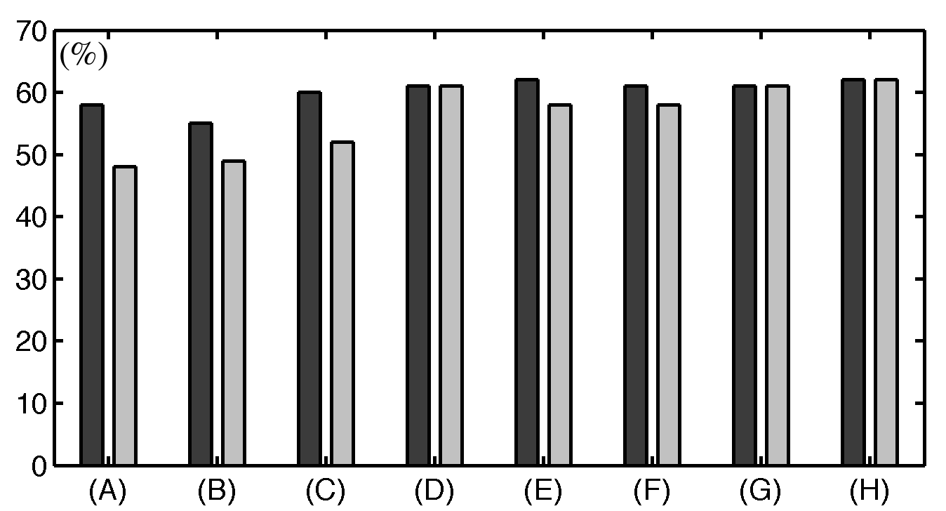
The results of the numerical experiments have been included in Figures 5–7. Figures 5 and 6 visualize the reconstructions together with the sets and for permittivity distributions (I) and (II), respectively. Figure 7 includes a bar plot of the ROA results.
The ROA was found to be systematically higher for (I) than (II). For each individual signal configuration, the greater or equal ROA value was obtained with (I). The range of variation was greater for distribution (II): the values observed were from 55 to 62 % and from 48 to 62 % for (I) and (II), respectively. The dense signal configurations (C), (D), (G), (H) with 2.1 spatial sampling rate (SR) yielded a better reconstruction quality than the sparse patterns (A), (B), (E), (F) (0.53 spatial SR). The ROA yielded by these groups was 60–62 % and 55–61 % for distribution (I) and 52–62 % and 48–58 % for (II), respectively. Furthermore, the difference between dense and sparse pattern under constant directional mixing was more pronounced in the case of one transmitter (A), (B), (C), (D) than in that of three (E), (F), (G), (H). For the former group, up to 24 % relative difference in ROA was observed, whereas for the latter one it stayed below 7 %.
The angular spacing of the transmitters had a notable effect on reconstruction quality in the case of single transmitter, where, e.g., the configurations (C) and (D) yielded the ROA of 52 and 61 %, respectively, for distribution (II). In the case of multiple transmitters, the effect of angular spacing was observed to be negligible. The number of transmitters and density of the data gathering points was found to be vital especially in the recovery of the surface layer of (II): the layer structure was virtually missing for sparse single-transmitter configurations.
IV Discussion
This study concentrated on computational methods and techniques for radio tomography of SPOs [1, 2, 3]. We introduced and tested a full waveform tomography approach which allows simulating orbiter-to-orbiter measurements, producing an inverse estimate for an arbitrary permittivity distribution and speeding up of computations for 3D imaging. The numerical experiments of this study focused, in particular, on (1) the sparsity/density of the measurement positions, (2) the number of transmitters in the satellite formation, (3) the directional variability of the signal paths, and (4) the recovery of (I) voids and (II) voids together with a surface layer, e.g. a dust or ice cover.
The reconstruction quality was observed to increase along with the number of both transmitter and receiver positions. For single transmitter signal configurations, spatial oversampling (SR 2.1) relative to NR yielded a significantly better quality compared to undersampling (SR 0.53). Reconstructing a surface layer was observed to be particularly difficult in the case of sparse data, when a single transmitter was used. Appropriate results were nevertheless obtained with three transmitters which suggests that a multiple transmitter setup is advantageous for a sparse distribution of measurement points, supporting our previous findings for multiple sources (landers) and sparse data [26, 45]. In a real application context, several different in situ constraints can lead to undersampling including the finite time and energy resources, the restricted signal bandwith, as well as the limited control of a satellite formation [46, 47, 48]. One obvious challenge is the slow satellite movement due to the weakness of the gravity field. Consequently, it is very likely that the inversion methodology will need to rely on sparse undersampled data.
In order to model the effect of orbiter movement on the reconstruction quality, we tested two different values for the angular spacing of the transmitter positions. Based on the results, this is a significant effect that needs to be taken into consideration in the mission design phase. Furthermore, it seems that the use of multiple transmitters can be advantageous in order to minimize this effect. It is also obvious that generating synthetic [15] data based on realistic orbiter movement in three dimensions is an important topic that deserves future research.
The multiresolution and incomplete Cholesky speedups [30, 33] were found to be well-suited for the current tomography context. For inversion in three dimensions, both of these techniques can be necessary extensions of our basic approach in order to achieve a reasonable computation time and compact memory usage. The incomplete Cholesky solver applied for the mass matrix was found to yield fast and reliable results, when fixing the level of filling (number of nonzeros) to 20 % compared to that of the full Cholesky decomposition. Choosing a lower level was observed to deteriorate the reconstruction quality. The multiresolution idea, i.e., the redefinition of the differentiated potential with respect to a coarse FE mesh, was successfully implemented going up one degree in the hierarchy of the nested meshes. Based on our initial tests, a multi-level hierarchy can be a feasible solution in order to further compress the time and memory consumption. The multiresolution speedup can be an essential tool to tackle the large and rapidly growing number of elements, which is of the order and for two- and three-dimensional elements of diameter , respectively. Namely, the speedup gain is exponential within the hierarchy of nested meshes, being comparable to the relative change in the number of elements (2D) or (3D) for a coarsening of degree .
The inversion strategy of this paper is based on total variation regularization [31, 32]. This technique was chosen as it, in principle, allows reconstructing an arbitrary permittivity distribution defined on the FE mesh. The values of the regularization parameters and were picked from the middle of the logarithmic interval of workable values which, based on our preliminary tests, led to approximately maximal overlap between the actual and reconstructed permittivities.
Further analysis of the robustness of the inversion could be conducted in the future. Additionally, implementing the present setting, e.g, within a Bayesian context [7] might also be a potential future direction, to allow more advanced analysis of the noise and enhanced formalism for the a priori information. Other future directions might concern realistic implementation of the present forward and inversion methodology. To support this kind of future research, the development of advanced asteroid models with various structures, such as cracks and porosity, would be essential. Features such as orbiter movement and the roughness of the body surface would be vital from the application point of view. Comparison between the current orbiter-to-orbiter measurement approach and, e.g., backscattering data would be important.
V Appendix
V-A Linearization
Differentiating the leap-frog formulas (14)–(15) with respect to at yields:
| (29) | |||||
| (30) | |||||
The last row of the second equation follows from the classical product (derivative) rule, since depends on . The formula for can be obtained via straightforward differentiation of . The product rule yields , that is
| (31) |
As the permittivity perturbation is of the form , the entries of can be expressed as
| (32) |
Hence, it follows that
| (33) |
if the -th element includes nodes and , otherwise . Substituting (31) into (30) the last row of (30) is of the form , where
| (34) |
Consequently, the system (29)–(30) can be written as
| (35) | |||||
| (36) | |||||
This is similar to (14)–(15) except from the source term that is specific, instead of a FE node, to the -th element in the FE mesh .
In this paper, the solution of (35)–(36) is found via the system (18)–(19) that has a point-specific source with , if and . This is essential for our deconvolution approach (Section II-B2) which relies on the reciprocity of the signal. Namely, the source term of (18)–(19) is monopolar similar to that of (14)–(15) and thus the reciprocity argument can be used.
Since , the source of (36) can be expressed as the sum of point-specific sources . It follows that since the wave equation is linear with respect to the source term, the solution of (35)–(36) can be obtained via the sum
| (37) |
where is a solution of (18)–(19). Due to the sparse structure of the vector differs from zero only if the -th node belongs to the element . For example, if the elements are triangular and the multiresolution speedup is used, i.e., if is defined w.r.t. , the non-zero source terms are , , where denote the three nodes associated with , and consequently, one can write
| (38) |
The whole procedure of linearization, as implemented in this paper, can be summarized as follows
- 1.
- 2.
- 3.
Inversion: Invert the data as explained in Section II-C.
V-B Inversion
In the algorithm (24), the matrix is diagonalizable as a symmetric matrix. If , then is positive definite and also invertible. Consequently, one can define
| (39) |
which substituted into (24) yields the following iteration [25, 26, 7]
| (40) |
This algorithm is closely related to alternating conditional minimization of the function
| (41) | |||||
in which , for . Since is a quadratic function with respect to , the conditional minimizer can be obtained through a least-squares approach of the form
| (42) |
At , the gradient of vanishes with respect to , i.e.,
| (43) |
The global minimum can be sought via the following alternating iteration.
- 1.
Set and . For a desired number of iterations repeat the following two steps.
- 2.
Find .
- 3.
Find .
In this algorithm, the sequence is identical to that of (40) and equals to the -th iterate of (24). If for some the pair is a global minimizer of , then, since , , it also minimizes the function
| (44) | |||||
Then, also is the minimizer of defined in (26), since with respect to the coordinate transform (39). The minimizer of is also the 1-norm regularized solution of the linearized inverse problem.
Acknowledgements
This work was supported by the Academy of Finland (Centre of Excellence in Inverse Problems Research).
References
- [1] I. Mann, A. Nakamura, and T. Mukai, Small Bodies in Planetary Systems, ser. Lecture Notes in Physics. Springer, 2008.
- [2] P. Michel, F. DeMeo, and W. Bottke, Asteroids IV, ser. Space Science Series. University of Arizona Press, 2015.
- [3] M. Kaasalainen and J. Durech, “Asteroid models for target selection and mission planning,” in Asteroids: Prospective Energy and Material Resources, V. Badescu, Ed. Springer-Verlag GmbH, 2013.
- [4] M. Kaasalainen, L. Lamberg, and K. Lumme, “Interpretation of lightcurves of atmosphereless bodies. ii. practical aspects of inversion,” A&A, vol. 259, no. 1, pp. 333–340, 1992.
- [5] M. Kaasalainen and L. Lamberg, “Inverse problems of generalized projection operators,” Inverse Problems, vol. 22, no. 3, pp. 749–769, 2006.
- [6] M. Kaasalainen, “Multimodal inverse problems: maximum compatibility estimate and shape reconstruction,” Inverse Problems and Imaging, vol. 5, no. 1, pp. 37–57, 2011.
- [7] J. P. Kaipio and E. Somersalo, Statistical and Computational Methods for Inverse Problems. Berlin: Springer, 2004.
- [8] M. Nabighian, Electromagnetic Methods in Applied Geophysics: Volume 1, Theory, ser. Electromagnetic Methods in Applied Geophysics: Applications Part A and Part B. Society of Exploration Geophysicists, 1988.
- [9] M. Benna, J.-P. Barriot, and W. Kofman, “A priori information required for a two or three dimensional reconstruction of the internal structure of a comet nucleus (CONSERT experiment),” Advances in Space Research, vol. 29, no. 5, pp. 715 – 724, 2002.
- [10] J. Belton, Mitigation of Hazardous Comets and Asteroids. Cambridge University Press, 2004.
- [11] A. Herique, J. Gilchrist, W. Kofman, and J. Klinger, “Dielectric properties of comet analog refractory materials,” Planetary and Space Science, vol. 50, no. 9, pp. 857–863, AUG 2002.
- [12] W. Kofman, A. Herique, Y. Barbin, J.-P. Barriot, V. Ciarletti, S. Clifford, P. Edenhofer, C. Elachi, C. Eyraud, J.-P. Goutail, E. Heggy, L. Jorda, J. Lasue, A.-C. Levasseur-Regourd, E. Nielsen, P. Pasquero, F. Preusker, P. Puget, D. Plettemeier, Y. Rogez, H. Sierks, C. Statz, H. Svedhem, I. Williams, S. Zine, and J. Van Zyl, “Properties of the 67p/churyumov-gerasimenko interior revealed by consert radar,” Science, vol. 349, no. 6247, 2015. [Online]. Available: http://www.sciencemag.org/content/349/6247/aab0639.abstract
- [13] W. Kofman, A. Herique, J.-P. Goutail, T. Hagfors, I. P. Williams, E. Nielsen, J.-P. Barriot, Y. Barbin, C. Elachi, P. Edenhofer, A.-C. Levasseur-Regourd, D. Plettemeier, G. Picardi, R. Seu, and V. Svedhem, “The comet nucleus sounding experiment by radiowave transmission (CONSERT): A short description of the instrument and of the commissioning stages,” Space Science Reviews, vol. 128, no. 1-4, pp. 413 – 432, 2007.
- [14] W. Kofman, A. Herique, and J. Goutail, “CONSERT experiment: Description and performances in view of the new target,” in New Rosetta Targets: Observations, Simulations and Instrument Performances, ser. Astrophysics and Space Science Library, L. Colangeli, E. Epifani, and P. Palumbo, Eds., vol. 311. Dordrecht, Netherlands: Springer, 2004, Proceedings Paper, pp. 237–256.
- [15] M. Benna, J.-P. Barriot, W. Kofman, and Y. Barbin, “Generation of 3-d synthetic data for the modeling of the CONSERT experiment (the radiotomography of comet 67p/churyumov-gerasimenko),” Antennas and Propagation, IEEE Transactions on, vol. 52, no. 3, pp. 709 – 716, march 2004.
- [16] W. Kofman, Y. Barbin, J. Klinger, A.-C. Levasseur-Regourd, J.-P. Barriot, A. Herique, T. Hagfors, E. Nielsen, and E. Gr “Comet nucleus sounding experiment by radiowave transmission,” Advances in Space Research, vol. 21, no. 11, pp. 1589 – 1598, 1998.
- [17] A. Herique, A. Barucci, J. Biele, T.-M. Ho, W. Kofman, C. Krause, P. Michel, D. Plettemeier, J. Y. Prado, J. C. Souyris, S. Zine, and S. Ulamec, “ASSERT : A Radar Tomography of Asteroids,” in EPSC-DPS Joint Meeting 2011, Oct. 2011, p. 924.
- [18] ——, “Radar Tomography of Asteroids,” in EPSC-DPS Joint Meeting 2011, Oct. 2011, p. 920.
- [19] A. Herique, D. Plettemeier, W. Kofman, S. Ulamec, J. Biele, J. Goutail, P. Beck, J. Lassue, A. Barucci, and P. Michel, “CONSERT for Asteroid - radar tomography of Near Earth Asteroid,” in EGU General Assembly 2010, May 2010, p. 11011.
- [20] A. Herique, W. Kofman, T. Hagfors, G. Caudal, and J.-P. Ayanides, “A characterization of a comet nucleus interior:inversion of simulated radio frequency data,” Planet. Space Sci., vol. 47, pp. 885–904, Jun. 1999.
- [21] D. Landmann, D. Plettemeier, C. Statz, F. Hoffeins, U. Markwardt, W. Nagel, A. Walther, A. Herique, and W. Kofman, “Three-dimensional reconstruction of a comet nucleus by optimal control of maxwell’s equations: A contribution to the experiment CONSERT onboard space craft Rosetta,” in Radar Conference, 2010 IEEE, may 2010, pp. 1392 –1396.
- [22] E. Nielsen, W. Engelhardt, B. Chares, L. Bemmann, M. Richards, F. Backwinkel, D. Plettemeier, P. Edenhofer, Y. Barbin, J. Goutail, W. Kofman, and L. Svedhem, “Antennas for sounding of a cometary nucleus in the Rosetta mission,” in Eleventh International Conference on Antennas and Propagation, Vols 1 and 2, ser. IEE Conference Publications, no. 480. 379 THORNALL ST, EDISON, NJ 08837 USA: Inst Electrical Engineers Inspec INC, 2001, Proceedings Paper, pp. 436–441.
- [23] J.-P. Barriot, W. Kofman, A. Herique, S. Leblanc, and A. Portal, “A two dimensional simulation of the CONSERT experiment (radio tomography of comet wirtanen),” Advances in Space Research, vol. 24, no. 9, pp. 1127 – 1138, 1999.
- [24] S. Pursiainen and M. Kaasalainen, “Iterative alternating sequential (IAS) method for radio tomography of asteroids in 3D,” Planetary and Space Science, vol. 78, 2013.
- [25] ——, “Detection of anomalies in radio tomography of asteroids: Source count and forward errors,” Planetary and Space Science, vol. 99, no. 0, pp. 36 – 47, 2014.
- [26] ——, “Sparse source travel-time tomography of a laboratory target: accuracy and robustness of anomaly detection,” p. 114016, 2014.
- [27] D. J. Daniels, Ground Penetrating Radar (2nd Edition). Stevenage: Institution of Engineering and Technology, 2004.
- [28] V. Agrawal, Satellite Technology: Principles and Applications. Wiley, 2014.
- [29] J. B. Schneider, Understanding the FDTD Method. John B. Schneider, 2012. [Online]. Available: http://www.eecs.wsu.edu/ schneidj/ufdtd/
- [30] D. Braess, Finite Elements: Theory, Fast Solvers, and Applications in Solid Mechanics. Cambridge University Press, 2007.
- [31] O. Scherzer, M. Grasmair, H. Grossauer, M. Haltmeier, and F. Lenzen, Variational Methods in Imaging, ser. Applied Mathematical Sciences. Springer New York, 2008.
- [32] W. Stefan, Total Variation Regularization for Linear Ill-posed Inverse Problems: Extensions and Applications. Arizona State University, 2008.
- [33] G. Golub and C. van Loan, Matrix Computations. Baltimore: The John Hopkins University Press, 1989.
- [34] L. Evans, Partial Differential Equations, ser. Graduate studies in mathematics. American Mathematical Society, 1998.
- [35] A. Bossavit and L. Kettunen, “Yee-like schemes on a tetrahedral mesh, with diagonal lumping,” International Journal of Numerical Modelling: Electronic Networks, Devices and Fields, vol. 12, no. 1-2, pp. 129–142, 1999.
- [36] K. Yee, “Numerical solution of initial boundary value problems involving maxwell’s equations in isotropic media,” Antennas and Propagation, IEEE Transactions on, vol. 14, no. 3, pp. 302–307, 1966.
- [37] C. Altman and K. Suchy, Reciprocity, Spatial Mapping and Time Reversal in Electromagnetics, ser. Developments in Electromagnetic Theory and Applications. Springer Netherlands, 1991.
- [38] J. L. Davis and A. P. Annan, “Ground penetrating radar for high resolution mapping of soil and rock stratigraphy,” Geoscience Canada, vol. 37, no. 5, pp. 531–551, 1989.
- [39] J. Irving and R. Knight, “Numerical modeling of ground-penetrating radar in 2-D using MATLAB,” Computers & Geosciences, vol. 32, no. 9, pp. 1247 – 1258, 2006.
- [40] F. J. Harris, “On the use of windows for harmonic analysis with the discrete fourier transform,” Proceedings of the IEEE, vol. 66, no. 1, pp. 51–83, 1978.
- [41] A. H. Nuttall, “Some windows with very good sidelobe behavior,” IEEE Transactions on Acoustics, Speech, Signal Processing, vol. ASSP-29, no. 1, pp. 84–91, 1981.
- [42] R. P. Binzel and W. Kofman, “Internal structure of near-earth objects,” Comptes Rendus Physique, vol. 6, no. 3, pp. 321–326, 2005.
- [43] J. Francke and V. Utsi, “Advances in long-range gpr systems and their applications to mineral exploration, geotechnical and static correction problems,” First Break, vol. 27, no. 7, pp. 85–93, 2009.
- [44] D. Colton and R. Kress, Inverse Acoustic and Electromagnetic Scattering Theory, ser. Applied Mathematical Sciences. Springer, 1998.
- [45] S. Pursiainen and M. Kaasalainen, “Electromagnetic 3d subsurface imaging with source sparsity for a synthetic object,” Inverse Problems, vol. 31, no. 12, p. 125004, 2015. [Online]. Available: http://stacks.iop.org/0266-5611/31/i=12/a=125004
- [46] D. Miller, A. Saenz-Otero, J. Wertz, A. Chen, G. Berkowski, C. Brodel, S. Carlson, D. Carpenter, S. Chen, and S. Cheng, “SPHERES: A testbed for long duration satellite formation flying in micro-gravity conditions,” ADVANCES IN THE ASTRONAUTICAL SCIENCES, vol. 105, pp. 167–180, 2000.
- [47] H.-H. Yeh and A. Sparks, “Geometry and control of satellite formations,” in American Control Conference, 2000. Proceedings of the 2000, vol. 1, no. 6, Sep 2000, pp. 384–388 vol.1.
- [48] R. Pongvthithum, S. M. Veres, S. B. Gabriel, and E. Rogers, “Universal adaptive control of satellite formation flying,” International Journal of Control, vol. 78, pp. 45–52, 2005.
![[Uncaptioned image]](1608.06566v1/pursiainen.jpg) |
Sampsa Pursiainen received his MSc(Eng) and PhD(Eng) degrees (Mathematics) in the Helsinki University of Technology (Aalto University since 2010), Espoo, Finland, in 2003 and 2009. He focuses on various forward and inversion techniques of applied mathematics. In 2010–11, he stayed at the Department of Mathematics, University of Genova, Italy collaborating also with the Institute for Biomagnetism and Biosignalanalysis (IBB), University of Münster, Germany. In 2012–15, he worked at the Department of Mathematics and Systems Analysis, Tampere University of Technology Finland and also at the Department of Mathematics, Tampere University of Technology, Finland, where he currently holds an Assistant Professor position. |
![[Uncaptioned image]](1608.06566v1/kaasalainen.jpg) |
Prof. Mikko Kaasalainen obtained his DPhil at Oxford in 1994, and he has been professor of applied mathematics at Tampere University of Technology since 2009. His main research fields are inverse problems and mathematical modelling, with interdisciplinary application projects ranging from biology to galactic dynamics. He is the vice director of the Centre of Excellence in Inverse Problems funded by the Academy of Finland. The website of his research group at TUT is at math.tut.fi/inversegroup |