跳到论文正文
W Papers独立论文阅读器 arXiv:1608.06041 论文正文 计算阅读时间 · 0%
引用这篇论文根据当前论文元数据生成,正式投稿前建议核对。


License: arXiv.org perpetual non-exclusive license
arXiv:1608.06041v1 [cs.IT] 22 Aug 2016

Hybrid Duplex Switching in Heterogeneous NetworksThanks:  W. Tang, S. Feng, Y. Liu, and Y. Ding are with School of Electronic and Information Engineering, South China University of Technology, Guangzhou 510641, China (e-mail: tang.weijun@mail.scut.edu.cn, {fengsl, eeyliu, eeyhding}@scut.edu.cn).

Weijun Tang, Suili Feng, Yuan Liu, and Yuehua Ding Affiliation: 
Abstract

In this paper, a novel hybrid-duplex scheme based on received power is proposed for heterogeneous networks (HetNets). In the proposed scheme, the duplex mode (half- or full-duplex) of each user is switchable according to the received power from its serving base station (BS). The signal-to-interference-plus-noise-ratio (SINR) and spectral efficiency are analyzed for both downlink and uplink channels by using the tools of inhomogeneous Poisson point process. Furthermore, determining power threshold for duplex mode switching is investigated for sum rate maximization, which is formulated as a nonlinear integer programming problem and a greedy algorithm is proposed to solve this problem. The theoretical analysis and the proposed algorithm are evaluated by numerical simulations. Simulation results show that the proposed hybrid-duplex scheme outperforms the half-duplex or full-duplex HetNet schemes.

Index Terms: 
Heterogeneous networks, full-duplex, stochastic geometry, inhomogeneous Poisson point process.

I Introduction

Due to the overwhelming crosstalk between the transmitter and the receiver circuits, time division duplexing (TDD) and frequency division duplexing (FDD) are commonly used in current wireless systems. As half-duplex techniques TDD/FDD split a common pool of resources into two subsets for forward and reverse links respectively. Such orthogonal resource separation in either temporal or spectral domain might restrict the system performance. To overcome the bottleneck, full-duplex is believed to be a promising technology, which enables simultaneous transmission and reception on the same frequency for a device. Thus, the system capacity is significantly improved by doubling spectrum efficiency [1]. Unfortunately, the crosstalk, known as self-interference (SI), could be billions of times (100100 dB+) stronger than the desired signal received over the air [2], which prevents full-duplex from engineering application. Thanks to [3, 4], a great improvement has been made in self-interference cancellation (SIC). Especially, in [4], the SIC capacity up to −122-122 dB is achieved over 2020 MHz band. These progresses bring in-band full-duplex into practice.

Progress in SIC encourages further researches of full-duplex in cellular networks, such as [5, 6, 7, 8]. With perfect SIC, [5] investigated a network consisting of full-duplex base stations (BSs) and half-duplex users, whose average user rate was studied by using stochastic geometry. Under the assumption of imperfect SIC, [6] derived the closed-form expressions for outage probability and achievable sum rate in a single cell consisting of a full-duplex BS and two half-duplex users. Both full-duplex BSs and users were considered in [7] using stochastic geometry and the outage probability was studied. In [8], a greedy algorithm for joint user selection and power allocation was proposed for multi-cell networks. It was shown that scheduling policies greatly impact the system performance. [5, 6, 9, 7, 8] concentrated on homogeneous cellular networks. For heterogeneous networks (HetNets) supporting explosive growth of mobile service, [10, 11] analyzed the downlink SINR in KK-tier HetNets. The authors of [12] proposed hybrid full/half-duplex HetNets where the BSs operated in either downlink half-duplex mode or bidirectional full-duplex mode under a predefined probability and all users in a cell used the same duplex mode. However, as pointed out in [13], the point process of uplink interfering users is not a PPP but a Poisson-Voronoi perturbed lattice. The authors in [14] proposed an inhomogeneous PPP model to capture the nature of such point process, where the intensity measure functions of interfering users were derived by considering user association. The inhomogeneous PPP model was also adopted in [15] to analyze the uplink performance in HetNets with power control.

To the best of our knowledge, HetNets whose users are free to switch the duplex modes have not been considered yet, which is the motivation of this paper. The main contributions of this paper are:

  1. 1.

    A novel hybrid-duplex scheme based on the received power is proposed. This is motivated by our analysis which reveals that, with imperfect SIC, half-duplex outperforms full-duplex if the downlink received power is lower than a certain threshold. In our paper, each user is capable of half-duplex or full-duplex operation according to its received signal power. However, reference [12] considered that all users in a same cell operated in either half-duplex or full-duplex mode. The simulations show that our proposed scheme significantly outperforms the scheme in [12].

  2. 2.

    The threshold for duplex mode switching is discussed. The threshold selection problem is formulated as a nonlinear integer programming for sum rate maximization. A greedy algorithm is proposed for solving the problem.

  3. 3.

    Both downlink and uplink analysis are based on inhomogeneous PPP which is more realistic than homogeneous PPP considered in [12].

  4. 4.

    Valuable insights are provided for practical designs. In particular, full-duplex would degrade SINR performance with RSI and large inter-cell interference. The downlink spectral efficiency is doubled by full-duplex with the sacrifices of uplink performance.

The rest of the paper is organized as follows. Section II presents the hybrid-duplex HetNet model. Section III provides the analytical results. The optimization problem and the numerical results are shown in Section IV and Section V, respectively. Section VI summarizes this paper.

II System Model

Refer to caption
Fig. 1: A two-tier hybrid-duplex heterogeneous networks.

We consider a two-tier network as shown in Fig. 1. The BS locations of tier kk (k=1,2k=1,2) are distributed as an independent homogeneous Poisson point process (PPP) Φk\Phi_{k} with density λk\lambda_{k}. Without loss of generality, we let the macro cells be tier 1 and the small cells be tier 2. The locations of users (denoted by 𝒰\mathcal{U}) follow an independent PPP Φu\Phi_{u} with density λu\lambda_{u}. Every BS of tier kk has the same transmit power {Pk}k=1,2\{P_{k}\}_{k=1,2} over the bandwidth WW, while the transmit power of the users is PuP_{u}. Both BSs and users are full-duplex capable. Considering imperfect SIC, the residual self-interference (RSI) of the BSs in the two tiers and the users are denoted as {R​S​Ik}k=1,2\{RSI_{k}\}_{k=1,2} and R​S​IuRSI_{u}, respectively. The small-scale fading is assumed to be Rayleigh distribution with unit power. The path loss is assumed as l⁡(d)=d−αl(d)=d^{-\alpha}, where dd is the propagation distance, and α>2\alpha>2 is the path loss exponent. For simplicity and tractability, shadowing is omitted here. Note that shadow fading can be approximately modeled by the randomness of the node locations [16]. Good approximations are obtained for a realistic assumption (logarithm standard deviation of the shadowing greater than 1010 dB) in many urban scenarios [17].

TABLE I: Notation Summary
Notation Description
Φk,ΦkFD,ΦkHD\Phi_{k},\Phi_{k}^{\text{FD}},\Phi_{k}^{\text{HD}}
Point process of BSs / full-duplex BSs /
half-duplex BSs in tier kk
Φu,Φu,kFD,Φu,kHD\Phi_{u},\Phi_{u,k}^{\text{FD}},\Phi_{u,k}^{\text{HD}}
Point process of users / full-duplex users /
half-duplex users in tier kk
λk;λu\lambda_{k};\lambda_{u}
Density of BSs in tier kk;
density of mobile users
Pk;PuP_{k};P_{u}
Transmit power of BSs in tier kk;
transmit power of users
R​S​Ik;R​S​IuRSI_{k};RSI_{u}
RSI of the BSs in tier kk; RSI of the users
γk\gamma_{k}
Received power threshold of tier kk
α;W\alpha;W
Path loss exponent; spectrum bandwidth
DkD_{k}
Distance from the typical user
to its closest BS in tier kk
DkFD,DkHDD_{k}^{\text{FD}},D_{k}^{\text{HD}}
Transmit distances between the typical user
and its serving BS in tier kk
Di,jD_{i,j}
Distance between node ii and node jj
hi,jh_{i,j}
Small scale fading between node ii and node jj
σ2\sigma^{2}
Thermal noise power
𝒜k,𝒜kFD,𝒜kHD\mathcal{A}_{k},\mathcal{A}_{k}^{\text{FD}},\mathcal{A}_{k}^{\text{HD}}
Association probabilities of the typical user
to tier kk
It,ki​,D,It,ki​,UI_{t,k}^{i\text{,D}},I_{t,k}^{i\text{,U}}
Cumulative interference on channel ii
from tier tt to tier kk
θki​,FD,D,θki​,FD,U,θki​,HD\theta_{k}^{i\text{,FD,D}},\theta_{k}^{i\text{,FD,U}},\theta_{k}^{i\text{,HD}}
SINRs on channel ii of a typical user in tier kk
λk,tBS,FD,D,λk,tBS,HD,D\lambda_{k,t}^{\text{BS,FD,D}},\lambda_{k,t}^{\text{BS,HD,D}},
λk,tBS,FD,U,λk,tBS,FD,U\lambda_{k,t}^{\text{BS,FD,U}},\lambda_{k,t}^{\text{BS,FD,U}}
Intensity measure functions of interfering BSs
λk,tUser,FD,D,λk,tUser,HD,D\lambda_{k,t}^{\text{User,FD,D}},\lambda_{k,t}^{\text{User,HD,D}},
λk,tUser,FD,U,λk,tUser,FD,U\lambda_{k,t}^{\text{User,FD,U}},\lambda_{k,t}^{\text{User,FD,U}}
Intensity measure functions of interfering users
𝒞ki​,FD,D,𝒞ki​,FD,U,𝒞ki​,HD\mathcal{C}_{k}^{i\text{,FD,D}},\mathcal{C}_{k}^{i\text{,FD,U}},\mathcal{C}_{k}^{i\text{,HD}}
SINR distributions on channel ii
of a typical user in tier kk
Ski​,FD,D,Ski​,FD,U,Ski​,HD,S_{k}^{i\text{,FD,D}},S_{k}^{i\text{,FD,U}},S_{k}^{i\text{,HD}},
Spectral efficiency on channel ii
of a typical user in tier kk

We assume that a user is associated with the BS that provides the maximum average downlink received power as in Long Term Evolution (LTE) [18]. Let {Dk}\{D_{k}\} denote the distance from a typical user to its closest BS in tier kk. The typical user is associated with the BS of tier kk if

k=argt⁡max⁡{Pt​Dt−α,t=1,2}.k=\arg_{t}\max\{P_{t}D_{t}^{-\alpha},t=1,2\}. (1)

After the cell association, the users’ duplex modes are scheduled based on the received signal power. We denote {γk}k=1,2\{\gamma_{k}\}_{k=1,2} as the received power thresholds. If the average downlink received signal power of a macro user is greater than or equal to the threshold of tier 11, i.e. P1​D1−α≥γ1P_{1}D_{1}^{-\alpha}\geq\gamma_{1}, the user is scheduled as a full-duplex user. Otherwise, if P1​D1−α<γ1P_{1}D_{1}^{-\alpha}<\gamma_{1}, the user communicates with its serving BS in half-duplex mode. For a small cell user, the case is similar except that the received power thresholds is γ2\gamma_{2}. The reason behind such a duplex mode selection policy is that, with imperfect SIC, using full-duplex mode might not benefit the users with low received signal power. Hence, the users suffering strong downlink received power are scheduled in full-duplex mode, otherwise, the users are in half-duplex mode. More details about the hybrid-duplex mode please refer to Appendix A.

According to the discussion above, the user set 𝒰\mathcal{U} can be divided into four disjoint sets:

{𝒰kFD,if ​Dk≤Dk¯​(PkPk¯)1/α​ and ​Dk≤(Pkγk)1/α𝒰kHD,if ​Dk≤Dk¯​(PkPk¯)1/α​ and ​Dk>(Pkγk)1/α,k=1,2,\begin{cases}\mathcal{U}_{k}^{\text{FD}},\text{if }D_{k}\leq D_{\bar{k}}\left(\frac{P_{k}}{P_{\bar{k}}}\right)^{1/\alpha}\text{ and }D_{k}\leq\left(\frac{P_{k}}{\gamma_{k}}\right)^{1/\alpha}\\ \mathcal{U}_{k}^{\text{HD}},\text{if }D_{k}\leq D_{\bar{k}}\left(\frac{P_{k}}{P_{\bar{k}}}\right)^{1/\alpha}\text{ and }D_{k}>\left(\frac{P_{k}}{\gamma_{k}}\right)^{1/\alpha}\\ \end{cases},k=1,2, (2)

where k¯=2\bar{k}=2 if k=1k=1 and k¯=1\bar{k}=1 if k=2k=2. 𝒰1FD\mathcal{U}_{1}^{\text{FD}} and 𝒰2FD\mathcal{U}_{2}^{\text{FD}} are the full-duplex user sets in macro cells and small cells, respectively. Similarly, 𝒰1HD\mathcal{U}_{1}^{\text{HD}} and 𝒰2HD\mathcal{U}_{2}^{\text{HD}} denote the half-duplex user sets in two tiers. Furthermore, we define 𝒰1=𝒰1FD∪𝒰1HD\mathcal{U}_{1}=\mathcal{U}_{1}^{\text{FD}}\cup\mathcal{U}_{1}^{\text{HD}} and 𝒰2=𝒰2FD∪𝒰2HD\mathcal{U}_{2}=\mathcal{U}_{2}^{\text{FD}}\cup\mathcal{U}_{2}^{\text{HD}} as the user sets of macro cells and small cells, respectively. Obviously, the typical user is in tier kk if Dk≤Dk¯​(PkPk¯)1/αD_{k}\leq D_{\bar{k}}\left(\frac{P_{k}}{P_{\bar{k}}}\right)^{1/\alpha}.

In this paper, we assume that the users (including full-duplex and half-duplex users) in a cell share the resources equally without intra-cell interference (but inter-cell interference exists due to full spectrum reuse), which can be done by the round-robin scheduling. Besides, the resources (e.g. time or frequency) in a cell are divided into two orthogonal parts equally: the uplink channel and the downlink channel. The two channels are for half-duplex users with uplink and downlink traffic respectively, while the full-duplex users communicate with their serving BSs bidirectionally on both channels. We call the downlink channel as channel 11 and the uplink channel as channel 22 in the rest of this paper. Further, the infinite backlogged data is assumed, such that the BSs and users always have data to transmit.

We denote DkFDD_{k}^{\text{FD}} and DkHDD_{k}^{\text{HD}} as the transmit distances between the typical user and its serving BS (called the tagged BS) when it is scheduled as a full-duplex user and a half-duplex user in tier kk, respectively. The SINRs on channel 11 of the typical user in tier kk can be expressed as

θk1​,FD,D\displaystyle\theta_{k}^{1\text{,FD,D}} =Pk​hb0,u0​(DkFD)−αR​S​Iu+∑t=1,2It,k1​,D+σ2,\displaystyle=\frac{P_{k}h_{b_{0},u_{0}}(D_{k}^{\text{FD}})^{-\alpha}}{RSI_{u}+\sum\limits_{t=1,2}I_{t,k}^{1\text{,D}}+\sigma^{2}}, (3)
θk1​,FD,U\displaystyle\theta_{k}^{1\text{,FD,U}} =Pu​hu0,b0​(DkFD)−αR​S​Ik+∑t=1,2It,k1​,U+σ2,\displaystyle=\frac{P_{u}h_{u_{0},b_{0}}(D_{k}^{\text{FD}})^{-\alpha}}{RSI_{k}+\sum\limits_{t=1,2}I_{t,k}^{1\text{,U}}+\sigma^{2}}, (4)
θk1​,HD\displaystyle\theta_{k}^{1\text{,HD}} =Pk​hb0,u0​(DkHD)−α∑t=1,2It,k1​,D+σ2,\displaystyle=\frac{P_{k}h_{b_{0},u_{0}}(D_{k}^{\text{HD}})^{-\alpha}}{\sum\limits_{t=1,2}I_{t,k}^{1\text{,D}}+\sigma^{2}}, (5)

where θk1​,FD,D\theta_{k}^{1\text{,FD,D}}, θk1​,FD,U\theta_{k}^{1\text{,FD,U}} are the downlink and uplink SINRs if the typical user is a full-duplex user in tier kk, respectively. θk1​,HD\theta_{k}^{1\text{,HD}} is the downlink SINR if the typical user is a half-duplex user. hi,j∼exp⁡(1)h_{i,j}\sim\exp(1) is the small-scale fading from node ii to node jj. b0b_{0} is denoted as the tagged BS, and u0u_{0} is the typical user. σ2\sigma^{2} is the noise power. It,k1​,DI_{t,k}^{1\text{,D}} and It,k1​,UI_{t,k}^{1\text{,U}} are the cumulative interference on channel 11 from tier tt (t=1,2t=1,2) to the typical users and the tagged BS in tier kk, respectively. It,k1​,DI_{t,k}^{1\text{,D}} and It,k1​,UI_{t,k}^{1\text{,U}} consist of the interference from other BSs and that from the interfering full-duplex users, which can be expressed as:

It,k1​,D=\displaystyle I_{t,k}^{1\text{,D}}= ∑bi∈ΦtFD∖b0Pt​hbi,u0​Dbi,u0−α+∑ui∈Φu,tFD∖u0Pu​hui,u0​Dui,u0−α\displaystyle\sum\limits_{b_{i}\in\Phi_{t}^{\text{FD}}\setminus b_{0}}P_{t}h_{b_{i},u_{0}}D_{b_{i},u_{0}}^{-\alpha}+\sum\limits_{u_{i}\in\Phi_{u,t}^{\text{FD}}\setminus u_{0}}P_{u}h_{u_{i},u_{0}}D_{u_{i},u_{0}}^{-\alpha}
+∑bi∈ΦtHD∖b0Pthbi,u0Dbi,u0−α,\displaystyle+\sum\limits_{b_{i}\in\Phi_{t}^{\text{HD}}\setminus b_{0}}P_{t}h_{b_{i},u_{0}}D_{b_{i},u_{0}}^{-\alpha}, (6)
It,k1​,U=\displaystyle I_{t,k}^{1\text{,U}}= ∑bi∈ΦtFD∖b0Pt​hbi,b0​Dbi,b0−α+∑ui∈Φu,tFD∖u0Pu​hui,b0​Dui,b0−α\displaystyle\sum\limits_{b_{i}\in\Phi_{t}^{\text{FD}}\setminus b_{0}}P_{t}h_{b_{i},b_{0}}D_{b_{i},b_{0}}^{-\alpha}+\sum\limits_{u_{i}\in\Phi_{u,t}^{\text{FD}}\setminus u_{0}}P_{u}h_{u_{i},b_{0}}D_{u_{i},b_{0}}^{-\alpha}
+∑bi∈ΦtHD∖b0Pthbi,b0Dbi,b0−α,\displaystyle+\sum\limits_{b_{i}\in\Phi_{t}^{\text{HD}}\setminus b_{0}}P_{t}h_{b_{i},b_{0}}D_{b_{i},b_{0}}^{-\alpha}, (7)

where ΦtFD\Phi_{t}^{\text{FD}} denotes the BSs in tier tt (t=1,2t=1,2) that are scheduling full-duplex users, ΦtHD\Phi_{t}^{\text{HD}} is denoted as the BSs scheduling half-duplex users. ubiu_{b_{i}} is denoted as the interfering user in the BS bib_{i}. Φu,tFD\Phi_{u,t}^{\text{FD}} is the point process denoting the locations of full-duplex interfering users in tier tt. Di,jD_{i,j} is the distance between node ii and node jj.

Similarly, the SINRs on channel 22 of the typical user in tier kk are defined as

θk2​,FD,D\displaystyle\theta_{k}^{2\text{,FD,D}} =Pk​hb0,u0​(DkFD)−αR​S​Iu+∑t=1,2It,k2​,D+σ2,\displaystyle=\frac{P_{k}h_{b_{0},u_{0}}(D_{k}^{\text{FD}})^{-\alpha}}{RSI_{u}+\sum\limits_{t=1,2}I_{t,k}^{2\text{,D}}+\sigma^{2}}, (8)
θk2​,FD,U\displaystyle\theta_{k}^{2\text{,FD,U}} =Pu​hu0,b0​(DkFD)−αR​S​Ik+∑t=1,2It,k2​,U+σ2,\displaystyle=\frac{P_{u}h_{u_{0},b_{0}}(D_{k}^{\text{FD}})^{-\alpha}}{RSI_{k}+\sum\limits_{t=1,2}I_{t,k}^{2\text{,U}}+\sigma^{2}}, (9)
θk2​,HD\displaystyle\theta_{k}^{2\text{,HD}} =Pu​hu0,b0​(DkHD)−α∑t=1,2It,k2​,U+σ2,\displaystyle=\frac{P_{u}h_{u_{0},b_{0}}(D_{k}^{\text{HD}})^{-\alpha}}{\sum\limits_{t=1,2}I_{t,k}^{2\text{,U}}+\sigma^{2}}, (10)

where θk2​,FD,D\theta_{k}^{2\text{,FD,D}} and θk2​,FD,U\theta_{k}^{2\text{,FD,U}} are the full-duplex downlink and uplink SINR in tier kk, respectively. θk2​,HD\theta_{k}^{2\text{,HD}} is the half-duplex uplink SINR. It,k2​,DI_{t,k}^{2\text{,D}} and It,k2​,UI_{t,k}^{2\text{,U}} are the cumulative interference on channel 22 from tier tt to the typical users and its serving BS in tier kk, which can be expressed as:

It,k2​,D=\displaystyle I_{t,k}^{2\text{,D}}= ∑bi∈ΦtFD∖b0Pt​hbi,u0​Dbi,u0−α+∑ui∈Φu,tFD∖u0Pu​hui,u0​Dui,u0−α\displaystyle\sum\limits_{b_{i}\in\Phi_{t}^{\text{FD}}\setminus b_{0}}P_{t}h_{b_{i},u_{0}}D_{b_{i},u_{0}}^{-\alpha}+\sum\limits_{u_{i}\in\Phi_{u,t}^{\text{FD}}\setminus u_{0}}P_{u}h_{u_{i},u_{0}}D_{u_{i},u_{0}}^{-\alpha}
+∑ui∈Φu,tHD∖u0Puhui,u0Dui,u0−α,\displaystyle+\sum\limits_{u_{i}\in\Phi_{u,t}^{\text{HD}}\setminus u_{0}}P_{u}h_{u_{i},u_{0}}D_{u_{i},u_{0}}^{-\alpha}, (11)
It,k2​,U=\displaystyle I_{t,k}^{2\text{,U}}= ∑bi∈ΦtFD∖b0Pt​hbi,b0​Dbi,b0−α+∑ui∈Φu,tFD∖u0Pu​hui,b0​Dui,b0−α\displaystyle\sum\limits_{b_{i}\in\Phi_{t}^{\text{FD}}\setminus b_{0}}P_{t}h_{b_{i},b_{0}}D_{b_{i},b_{0}}^{-\alpha}+\sum\limits_{u_{i}\in\Phi_{u,t}^{\text{FD}}\setminus u_{0}}P_{u}h_{u_{i},b_{0}}D_{u_{i},b_{0}}^{-\alpha}
+∑ui∈Φu,tHD∖u0Puhui,b0Dui,b0−α,\displaystyle+\sum\limits_{u_{i}\in\Phi_{u,t}^{\text{HD}}\setminus u_{0}}P_{u}h_{u_{i},b_{0}}D_{u_{i},b_{0}}^{-\alpha}, (12)

where Φu,tHD\Phi_{u,t}^{\text{HD}} is the point process denoting the locations of half-duplex interfering users in tier tt. For ease of reading, the notations are summarized in Table I.

III Analytical Modeling

In this section, we show the analytical performance results of the proposed HetNets. First we derive the SINR distributions on channel ii (i∈{1,2}i\in\{1,2\}) of the typical user when it is scheduled as a full-duplex or half-duplex user, respectively. Then we define and derive the spectral efficiency.

III-A SINR Distributions

The SINR distributions on channel ii (i∈{1,2}i\in\{1,2\}) of the typical user are defined as

𝒞i​,FD,D​(T)\displaystyle\mathcal{C}^{i\text{,FD,D}}(T)
=∑k=1,2𝒜kFD​𝒞ki​,FD,D​(T)∑k=1,2𝒜kFD≜∑k=1,2𝒜kFD​ℙ​(θki​,FD,D>T)∑k=1,2𝒜kFD,\displaystyle=\frac{\sum\limits_{k=1,2}\mathcal{A}_{k}^{\text{FD}}\mathcal{C}_{k}^{i\text{,FD,D}}(T)}{\sum\limits_{k=1,2}\mathcal{A}_{k}^{\text{FD}}}\triangleq\frac{\sum\limits_{k=1,2}\mathcal{A}_{k}^{\text{FD}}\mathbb{P}(\theta_{k}^{i\text{,FD,D}}>T)}{\sum\limits_{k=1,2}\mathcal{A}_{k}^{\text{FD}}}, (13)
𝒞i​,FD,U​(T)\displaystyle\mathcal{C}^{i\text{,FD,U}}(T)
=∑k=1,2𝒜kFD​𝒞ki​,FD,U​(T)∑k=1,2𝒜kFD≜∑k=1,2𝒜kFD​ℙ​(θki​,FD,U>T)∑k=1,2𝒜kFD,\displaystyle=\frac{\sum\limits_{k=1,2}\mathcal{A}_{k}^{\text{FD}}\mathcal{C}_{k}^{i\text{,FD,U}}(T)}{\sum\limits_{k=1,2}\mathcal{A}_{k}^{\text{FD}}}\triangleq\frac{\sum\limits_{k=1,2}\mathcal{A}_{k}^{\text{FD}}\mathbb{P}(\theta_{k}^{i\text{,FD,U}}>T)}{\sum\limits_{k=1,2}\mathcal{A}_{k}^{\text{FD}}}, (14)
𝒞i​,HD​(T)\displaystyle\mathcal{C}^{i\text{,HD}}(T)
=∑k=1,2𝒜kHD​𝒞ki​,HD​(T)∑k=1,2𝒜kHD≜∑k=1,2𝒜kHD​ℙ​(θki​,HD>T)∑k=1,2𝒜kHD,\displaystyle=\frac{\sum\limits_{k=1,2}\mathcal{A}_{k}^{\text{HD}}\mathcal{C}_{k}^{i\text{,HD}}(T)}{\sum\limits_{k=1,2}\mathcal{A}_{k}^{\text{HD}}}\triangleq\frac{\sum\limits_{k=1,2}\mathcal{A}_{k}^{\text{HD}}\mathbb{P}(\theta_{k}^{i\text{,HD}}>T)}{\sum\limits_{k=1,2}\mathcal{A}_{k}^{\text{HD}}}, (15)

where 𝒞ki​,FD,D​(T)\mathcal{C}_{k}^{i\text{,FD,D}}(T) and 𝒞ki​,FD,U​(T)\mathcal{C}_{k}^{i\text{,FD,U}}(T) are the downlink and uplink SINR distributions on channel ii of the typical user when it is a full-duplex user in tier kk, respectively. When the typical user is a half-duplex user in tier kk, the downlink SINR distribution on channel 11 is 𝒞k1​,HD​(T)\mathcal{C}_{k}^{1\text{,HD}}(T) and the uplink SINR distribution on channel 22 is 𝒞k2​,HD​(T)\mathcal{C}_{k}^{2\text{,HD}}(T). 𝒜kFD\mathcal{A}_{k}^{\text{FD}} and 𝒜kHD\mathcal{A}_{k}^{\text{HD}} are the association probabilities that the typical user is a full/half-duplex user in tier kk, respectively. ℙ⁡(X)\mathbb{P}(X) denotes the probability that event XX happens, and TT is the SINR threshold. Before obtaining the expressions of the SINR distributions, we first derive the association probabilities.

Lemma 1.

The association probabilities that the typical user is a full-duplex or half-duplex user in tier kk are

𝒜kFD=λk​Pk2/α​(1−exp⁡(−π​λk​δk2−π​λk¯​μk2​(δk)))λk​Pk2/α+λk¯​Pk¯2/α,\displaystyle\mathcal{A}_{k}^{\text{FD}}=\frac{\lambda_{k}P_{k}^{2/\alpha}\left(1-\exp\left(-\pi\lambda_{k}\delta_{k}^{2}-\pi\lambda_{\bar{k}}\mu_{k}^{2}(\delta_{k})\right)\right)}{\lambda_{k}P_{k}^{2/\alpha}+\lambda_{\bar{k}}P_{\bar{k}}^{2/\alpha}}, (16)
𝒜kHD=λk​Pk2/α​exp⁡(−π​λk​δk2−π​λk¯​μk2​(δk))λk​Pk2/α+λk¯​Pk¯2/α,\displaystyle\mathcal{A}_{k}^{\text{HD}}=\frac{\lambda_{k}P_{k}^{2/\alpha}\exp\left(-\pi\lambda_{k}\delta_{k}^{2}-\pi\lambda_{\bar{k}}\mu_{k}^{2}(\delta_{k})\right)}{\lambda_{k}P_{k}^{2/\alpha}+\lambda_{\bar{k}}P_{\bar{k}}^{2/\alpha}}, (17)

and the probability that a user is associated with tier kk is

𝒜k=𝒜kFD+𝒜kHD=λk​Pk2/αλk​Pk2/α+λk¯​Pk¯2/α,\mathcal{A}_{k}=\mathcal{A}_{k}^{\text{FD}}+\mathcal{A}_{k}^{\text{HD}}=\frac{\lambda_{k}P_{k}^{2/\alpha}}{\lambda_{k}P_{k}^{2/\alpha}+\lambda_{\bar{k}}P_{\bar{k}}^{2/\alpha}}, (18)

where δk≜(Pkγk)1/α\delta_{k}\triangleq\left(\frac{P_{k}}{\gamma_{k}}\right)^{1/\alpha} and μk(x)≜x(Pk¯Pk)1/α,k=1,2\mu_{k}(x)\triangleq x\left(\frac{P_{\bar{k}}}{P_{k}}\right)^{1/\alpha},k=1,2.

Proof:

Please see Appendix B. ∎

III-A1 Downlink SINR Distributions

Let us consider the downlink SINR distributions of the typical user. Note that each BS schedules its associated users independently. Hence, the probability that a BS in tier tt schedules a full-duplex user is 𝒜tFD𝒜t\frac{\mathcal{A}_{t}^{\text{FD}}}{\mathcal{A}_{t}}. According to the property of PPP [19], the BSs (ΦtFD\Phi_{t}^{\text{FD}}) scheduling full-duplex users form a PPP with a density of λtFD≜𝒜tFD𝒜t​λt\lambda_{t}^{\text{FD}}\triangleq\frac{\mathcal{A}_{t}^{\text{FD}}}{\mathcal{A}_{t}}\lambda_{t}. Similarly, ΦtHD\Phi_{t}^{\text{HD}} is a PPP with density λtHD≜𝒜tHD𝒜t​λt\lambda_{t}^{\text{HD}}\triangleq\frac{\mathcal{A}_{t}^{\text{HD}}}{\mathcal{A}_{t}}\lambda_{t}.

Due to the scheduling and association criteria, only one user per BS transmits on the same resource as the typical user. Therefore, {Φu,tFD}\{\Phi_{u,t}^{\text{FD}}\} and {Φu,tHD}\{\Phi_{u,t}^{\text{HD}}\} are not PPPs but Poisson-Voronoi perturbed lattice [13]. In addition, since the users may either be full- or half-duplex according to their received downlink average power, {ΦtFD}\{\Phi_{t}^{\text{FD}}\} and {ΦtHD}\{\Phi_{t}^{\text{HD}}\} are not PPPs, either. Moreover, there exists correlation between the typical user/tagged BS and the interfering nodes [14, 15]. Therefore, we adopt the similar approximation in [14] to characterize the processes as inhomogeneous PPPs.

Assumption 1.

When considering the downlink performance in tier kk, conditioned on the distance rr between the tagged BS and the typical user, the point processes are assumed to be Poisson with intensity measure functions as

ΦtFD:λk,tBS,FD,D​(y)=λtFD​(1−exp⁡(−λu​π​ζ2)),\displaystyle\Phi_{t}^{\text{FD}}:\lambda_{k,t}^{\text{BS,FD,D}}(y)=\lambda_{t}^{\text{FD}}\left(1-\exp(-\lambda_{u}\pi\zeta^{2})\right), (19)
ΦtHD:λk,tBS,HD,D​(y)={0,ζ≤δt,λtHD​(1−exp⁡(−λu​π​(ζ2−δt2))),ζ>δt,\displaystyle\Phi_{t}^{\text{HD}}:\lambda_{k,t}^{\text{BS,HD,D}}(y)=\begin{cases}0,\quad\zeta\leq\delta_{t},\\ \lambda_{t}^{\text{HD}}(1-\exp(-\lambda_{u}\pi(\zeta^{2}-\delta_{t}^{2}))),\zeta>\delta_{t},\end{cases} (20)
Φu,tFD:\displaystyle\Phi_{u,t}^{\text{FD}}: λk,tUser,FD,D​(y)\displaystyle\lambda_{k,t}^{\text{User,FD,D}}(y)
=λtFD​(1−exp⁡(−π​(r+y)2​λt​(PtPk)2/α)),\displaystyle=\lambda_{t}^{\text{FD}}\left(1-\exp\left(-\pi(r+y)^{2}\lambda_{t}(\frac{P_{t}}{P_{k}})^{2/\alpha}\right)\right), (21)
Φu,tHD:\displaystyle\Phi_{u,t}^{\text{HD}}: λk,tUser,HD,D​(y)\displaystyle\lambda_{k,t}^{\text{User,HD,D}}(y)
=λtHD​(1−exp⁡(−π​(r+y)2​λt​(PtPk)2/α)),\displaystyle=\lambda_{t}^{\text{HD}}\left(1-\exp\left(-\pi(r+y)^{2}\lambda_{t}(\frac{P_{t}}{P_{k}})^{2/\alpha}\right)\right), (22)

where yy is the distance to the typical user, and

ζ=r+ymax⁡{(PkPt)1/α−1,0}.\zeta=\frac{r+y}{\max\{(\frac{P_{k}}{P_{t}})^{1/\alpha}-1,0\}}. (23)

More details about these point processes please refer to Appendix C.

Theorem 1.

The downlink SINR distributions 𝒞k1​,FD,D\mathcal{C}_{k}^{1\text{,FD,D}}, 𝒞k1​,HD\mathcal{C}_{k}^{1\text{,HD}} and 𝒞k2​FD,D\mathcal{C}_{k}^{2\text{FD,D}} are (24), (25) and (26) on the top of page 55, respectively,

𝒞k1​,FD,D​(T)\displaystyle\mathcal{C}_{k}^{1\text{,FD,D}}(T) =2​π​λk𝒜kFD​∫0δkexp⁡(−TS​S​I​N​Rk,u​(r))​ℱ​(r)​∏t=k,k¯ℒΦtFD​(r,T)​ℒΦu,tFD​(r,T)​ℒΦtHD​(r,T)​𝑑r,\displaystyle=\frac{2\pi\lambda_{k}}{\mathcal{A}_{k}^{\text{FD}}}\int\limits_{0}^{\delta_{k}}\exp\left(-\frac{T}{SSINR_{k,u}(r)}\right)\mathcal{F}(r)\prod\limits_{t=k,\bar{k}}\mathcal{L}_{\Phi_{t}^{\text{FD}}}(r,T)\mathcal{L}_{\Phi_{u,t}^{\text{FD}}}(r,T)\mathcal{L}_{\Phi_{t}^{\text{HD}}}(r,T)dr, (24)
𝒞k1​,HD​(T)\displaystyle\mathcal{C}_{k}^{1\text{,HD}}(T) =2​π​λk𝒜kHD​∫δt∞exp⁡(−TS​N​Rk​(r))​ℱ​(r)​∏t=k,k¯ℒΦtFD​(r,T)​ℒΦu,tFD​(r,T)​ℒΦtHD​(r,T)​𝑑r,\displaystyle=\frac{2\pi\lambda_{k}}{\mathcal{A}_{k}^{\text{HD}}}\int\limits_{\delta_{t}}^{\infty}\exp\left(-\frac{T}{SNR_{k}(r)}\right)\mathcal{F}(r)\prod\limits_{t=k,\bar{k}}\mathcal{L}_{\Phi_{t}^{\text{FD}}}(r,T)\mathcal{L}_{\Phi_{u,t}^{\text{FD}}}(r,T)\mathcal{L}_{\Phi_{t}^{\text{HD}}}(r,T)dr, (25)
𝒞k2​,FD,D​(T)\displaystyle\mathcal{C}_{k}^{2\text{,FD,D}}(T) =2​π​λk𝒜kFD​∫0δtexp⁡(−TS​S​I​N​Rk,u​(r))​ℱ​(r)​∏t=k,k¯ℒΦtFD​(r,T)​ℒΦu,tFD​(r,T)​ℒΦu,tHD​(r,T)​𝑑r,\displaystyle=\frac{2\pi\lambda_{k}}{\mathcal{A}_{k}^{\text{FD}}}\int\limits_{0}^{\delta_{t}}\exp\left(-\frac{T}{SSINR_{k,u}(r)}\right)\mathcal{F}(r)\prod\limits_{t=k,\bar{k}}\mathcal{L}_{\Phi_{t}^{\text{FD}}}(r,T)\mathcal{L}_{\Phi_{u,t}^{\text{FD}}}(r,T)\mathcal{L}_{\Phi_{u,t}^{\text{HD}}}(r,T)dr, (26)
ℱ⁡(r)\displaystyle\mathcal{F}(r) =r​exp⁡(−π​λk​r2−π​λk¯​(μk​(r))2),\displaystyle=r\exp\left(-\pi\lambda_{k}r^{2}-\pi\lambda_{\bar{k}}(\mu_{k}(r))^{2}\right), (27)
ℒΦtFD​(r,T)\displaystyle\mathcal{L}_{\Phi_{t}^{\text{FD}}}(r,T) =exp(−2π∫Δk,t​(r)∞λk,tBS,FD,D(y)y(1−ℒh(Pt​T​rαPk​yα))dy),\displaystyle=\exp\left(-2\pi\int_{\Delta_{k,t}(r)}^{\infty}\lambda_{k,t}^{\text{BS,FD,D}}(y)y\left(1-\mathcal{L}_{h}\left(\frac{P_{t}Tr^{\alpha}}{P_{k}y^{\alpha}}\right)\right)dy\right), (28)
ℒΦtHD​(r,T)\displaystyle\mathcal{L}_{\Phi_{t}^{\text{HD}}}(r,T) =exp(−2π∫Δk,t​(r)∞λk,tBS,HD,D(y)y(1−ℒh(Pt​T​rαPk​yα))dy),\displaystyle=\exp\left(-2\pi\int_{\Delta_{k,t}(r)}^{\infty}\lambda_{k,t}^{\text{BS,HD,D}}(y)y\left(1-\mathcal{L}_{h}\left(\frac{P_{t}Tr^{\alpha}}{P_{k}y^{\alpha}}\right)\right)dy\right), (29)
ℒΦu,tFD​(r,T)\displaystyle\mathcal{L}_{\Phi_{u,t}^{\text{FD}}}(r,T) =exp(−2π∫max⁡{r​(PtPk)1/α−δt,0}∞λk,tUser,FD,D(y)y(1−ℒh(Pu​T​rαPk​yα))dy),\displaystyle=\exp\left(-2\pi\int_{\max\{r(\frac{P_{t}}{P_{k}})^{1/\alpha}-\delta_{t},0\}}^{\infty}\lambda_{k,t}^{\text{User,FD,D}}(y)y\left(1-\mathcal{L}_{h}\left(\frac{P_{u}Tr^{\alpha}}{P_{k}y^{\alpha}}\right)\right)dy\right), (30)
ℒΦu,tHD​(r,T)\displaystyle\mathcal{L}_{\Phi_{u,t}^{\text{HD}}}(r,T) =exp(−2π∫max⁡{δt​(PkPt)1/α−r,0}∞λk,tUser,HD,D(y)y(1−ℒh(Pu​T​rαPk​yα))dy).\displaystyle=\exp\left(-2\pi\int_{\max\{\delta_{t}(\frac{P_{k}}{P_{t}})^{1/\alpha}-r,0\}}^{\infty}\lambda_{k,t}^{\text{User,HD,D}}(y)y\left(1-\mathcal{L}_{h}\left(\frac{P_{u}Tr^{\alpha}}{P_{k}y^{\alpha}}\right)\right)dy\right). (31)


where Δk,t​(r)≜r​(PtPk)1/α\Delta_{k,t}(r)\triangleq r\left(\frac{P_{t}}{P_{k}}\right)^{1/\alpha}, ℒh​(s)=11+s\mathcal{L}_{h}(s)=\frac{1}{1+s} is the Laplace transform of h∼exp⁡(1)h\sim\exp(1). S​S​I​N​Rt,r​(d)≜Pt​d−αR​S​Ir+σ2SSINR_{t,r}(d)\triangleq\frac{P_{t}d^{-\alpha}}{RSI_{r}+\sigma^{2}}, is the signal-to-self-interference-plus-noise ratio (SSINR), and S​N​Rt​(d)≜Pt​d−ασ2SNR_{t}(d)\triangleq\frac{P_{t}d^{-\alpha}}{\sigma^{2}} is the signal-to-noise ratio (SNR).

Proof:

Please see Appendix D. ∎

III-A2 Uplink SINR Distributions

Adopting a similar approximation to that in the previous subsection, we approximate the point processes of interfering nodes’ locations as independent inhomogeneous PPPs.

Assumption 2.

When considering the uplink performance in tier kk, conditioned on the distance rr between the tagged BS and the typical user, the point processes are assumed to be Poisson with intensity measure functions as

ΦtFD:\displaystyle\Phi_{t}^{\text{FD}}: λk,tBS,FD,U​(y)=λtFD​(1−exp⁡(−λu​π​ζ2)),\displaystyle\lambda_{k,t}^{\text{BS,FD,U}}(y)=\lambda_{t}^{\text{FD}}\left(1-\exp(-\lambda_{u}\pi\zeta^{2})\right), (32)
ΦtHD:\displaystyle\Phi_{t}^{\text{HD}}: λk,tBS,HD,U​(y)\displaystyle\lambda_{k,t}^{\text{BS,HD,U}}(y)
={0,ζ≤δt,λtHD​(1−exp⁡(−λu​π​(ζ2−δt2))),ζ>δt,\displaystyle=\begin{cases}0,\quad\zeta\leq\delta_{t},\\ \lambda_{t}^{\text{HD}}\left(1-\exp\left(-\lambda_{u}\pi(\zeta^{2}-\delta_{t}^{2})\right)\right),\zeta>\delta_{t},\end{cases} (33)
Φu,tFD:\displaystyle\Phi_{u,t}^{\text{FD}}: λk,tUser,FD,D​(y)\displaystyle\lambda_{k,t}^{\text{User,FD,D}}(y)
=λtFD​(1−exp⁡(−π​y2​λt​(PtPk)2/α)),\displaystyle=\lambda_{t}^{\text{FD}}\left(1-\exp\left(-\pi y^{2}\lambda_{t}(\frac{P_{t}}{P_{k}})^{2/\alpha}\right)\right), (34)
Φu,tHD:\displaystyle\Phi_{u,t}^{\text{HD}}: λk,tUser,HD,U​(y)\displaystyle\lambda_{k,t}^{\text{User,HD,U}}(y)
=λtHD​(1−exp⁡(−π​y2​λt​(PtPk)2/α)),\displaystyle=\lambda_{t}^{\text{HD}}\left(1-\exp\left(-\pi y^{2}\lambda_{t}(\frac{P_{t}}{P_{k}})^{2/\alpha}\right)\right), (35)

where yy is the distance to the tagged BS, and

ζ=ymax⁡{(PkPt)1/α−1,0}.\zeta=\frac{y}{\max\{(\frac{P_{k}}{P_{t}})^{1/\alpha}-1,0\}}. (36)

The intensity measure functions above are obtained by similar process as that in Appendix C. Due to the limited place, the details are omitted.

Theorem 2.

The uplink SINR distributions 𝒞k1​,FD,U\mathcal{C}_{k}^{1\text{,FD,U}}, 𝒞k2​,FD,U\mathcal{C}_{k}^{2\text{,FD,U}} and 𝒞k2​,HD\mathcal{C}_{k}^{2\text{,HD}} are (37), (38), (39) on the top of page 66, respectively, where ℱ⁡(r)\mathcal{F}(r) is (27) on page 55.

𝒞k1​,FD,U​(T)\displaystyle\mathcal{C}_{k}^{1\text{,FD,U}}(T) =2​π​λk𝒜kFD​∫0δkexp⁡(−TS​S​I​N​Ru,k​(r))​ℱ​(r)​∏t=k,k¯ℒΦtFD​(r,T)​ℒΦu,tFD​(r,T)​ℒΦtHD​(r,T)​𝑑r,\displaystyle=\frac{2\pi\lambda_{k}}{\mathcal{A}_{k}^{\text{FD}}}\int\limits_{0}^{\delta_{k}}\exp\left(-\frac{T}{SSINR_{u,k}(r)}\right)\mathcal{F}(r)\prod\limits_{t=k,\bar{k}}\mathcal{L}_{\Phi_{t}^{\text{FD}}}(r,T)\mathcal{L}_{\Phi_{u,t}^{\text{FD}}}(r,T)\mathcal{L}_{\Phi_{t}^{\text{HD}}}(r,T)dr, (37)
𝒞k2​,FD,U​(T)\displaystyle\mathcal{C}_{k}^{2\text{,FD,U}}(T) =2​π​λk𝒜kFD​∫0δkexp⁡(−TS​S​I​N​Ru,k​(r))​ℱ​(r)​∏t=k,k¯ℒΦtFD​(r,T)​ℒΦu,tFD​(r,T)​ℒΦu,tHD​(r,T)​𝑑r,\displaystyle=\frac{2\pi\lambda_{k}}{\mathcal{A}_{k}^{\text{FD}}}\int\limits_{0}^{\delta_{k}}\exp\left(-\frac{T}{SSINR_{u,k}(r)}\right)\mathcal{F}(r)\prod\limits_{t=k,\bar{k}}\mathcal{L}_{\Phi_{t}^{\text{FD}}}(r,T)\mathcal{L}_{\Phi_{u,t}^{\text{FD}}}(r,T)\mathcal{L}_{\Phi_{u,t}^{\text{HD}}}(r,T)dr, (38)
𝒞k2​,HD​(T)\displaystyle\mathcal{C}_{k}^{2\text{,HD}}(T) =2​π​λk𝒜kHD​∫δk∞exp⁡(−TS​N​Ru​(r))​ℱ​(r)​∏t=k,k¯ℒΦtFD​(r,T)​ℒΦu,tFD​(r,T)​ℒΦu,tHD​(r,T)​𝑑r,\displaystyle=\frac{2\pi\lambda_{k}}{\mathcal{A}_{k}^{\text{HD}}}\int\limits_{\delta_{k}}^{\infty}\exp\left(-\frac{T}{SNR_{u}(r)}\right)\mathcal{F}(r)\prod\limits_{t=k,\bar{k}}\mathcal{L}_{\Phi_{t}^{\text{FD}}}(r,T)\mathcal{L}_{\Phi_{u,t}^{\text{FD}}}(r,T)\mathcal{L}_{\Phi_{u,t}^{\text{HD}}}(r,T)dr, (39)
ℒΦtFD​(r,T)\displaystyle\mathcal{L}_{\Phi_{t}^{\text{FD}}}(r,T) =exp(−2πpk,tI∫0Δk,t⁡(r)+rλk,tBS,FD,U(y)y(1−ℒh(Pt​T​rαPu​yα))dy\displaystyle=\exp\Bigg(-2\pi p_{k,t}^{I}\int_{0}^{\Delta_{k},t(r)+r}\lambda_{k,t}^{\text{BS,FD,U}}(y)y\left(1-\mathcal{L}_{h}\left(\frac{P_{t}Tr^{\alpha}}{P_{u}y^{\alpha}}\right)\right)dy
−2π∫Δk,t​(r)+r∞λk,tBS,FD,U(y)y(1−ℒh(Pt​T​rαPu​yα))dy),\displaystyle\qquad\qquad\qquad-2\pi\int_{\Delta_{k,t}(r)+r}^{\infty}\lambda_{k,t}^{\text{BS,FD,U}}(y)y\left(1-\mathcal{L}_{h}\left(\frac{P_{t}Tr^{\alpha}}{P_{u}y^{\alpha}}\right)\right)dy\Bigg), (40)
ℒΦtHD​(r,T)\displaystyle\mathcal{L}_{\Phi_{t}^{\text{HD}}}(r,T) =exp(−2πpk,tI∫0Δk,t⁡(r)+rλk,tBS,HD,U(y)y(1−ℒh(Pt​T​rαPu​yα))dy\displaystyle=\exp\Bigg(-2\pi p_{k,t}^{I}\int_{0}^{\Delta_{k},t(r)+r}\lambda_{k,t}^{\text{BS,HD,U}}(y)y\left(1-\mathcal{L}_{h}\left(\frac{P_{t}Tr^{\alpha}}{P_{u}y^{\alpha}}\right)\right)dy
−2π∫Δk,t​(r)+r∞λk,tBS,HD,U(y)y(1−ℒh(Pt​T​rαPu​yα))dy),\displaystyle\qquad\qquad\qquad-2\pi\int_{\Delta_{k,t}(r)+r}^{\infty}\lambda_{k,t}^{\text{BS,HD,U}}(y)y\left(1-\mathcal{L}_{h}\left(\frac{P_{t}Tr^{\alpha}}{P_{u}y^{\alpha}}\right)\right)dy\Bigg), (41)
ℒΦu,tFD​(r,T)\displaystyle\mathcal{L}_{\Phi_{u,t}^{\text{FD}}}(r,T) =exp(−2π∫max⁡{((PtPk)1/α−1)​r−δt,0}∞λk,tUser,FD,U(y)y(1−ℒh(T​rαyα))dy),\displaystyle=\exp\left(-2\pi\int_{\max\{((\frac{P_{t}}{P_{k}})^{1/\alpha}-1)r-\delta_{t},0\}}^{\infty}\lambda_{k,t}^{\text{User,FD,U}}(y)y\left(1-\mathcal{L}_{h}\left(\frac{Tr^{\alpha}}{y^{\alpha}}\right)\right)dy\right), (42)
ℒΦu,tHD​(r,T)\displaystyle\mathcal{L}_{\Phi_{u,t}^{\text{HD}}}(r,T) =exp(−2π∫(PkPt)1/α​δt∞λk,tUser,HD,U(y)y(1−ℒh(T​rαyα))dy),\displaystyle=\exp\left(-2\pi\int_{(\frac{P_{k}}{P_{t}})^{1/\alpha}\delta_{t}}^{\infty}\lambda_{k,t}^{\text{User,HD,U}}(y)y\left(1-\mathcal{L}_{h}\left(\frac{Tr^{\alpha}}{y^{\alpha}}\right)\right)dy\right), (43)
pk,tI\displaystyle p_{k,t}^{I} =1−(Pt1/αPt1/α+Pk1/α)2.\displaystyle=1-\left(\frac{P_{t}^{1/\alpha}}{P_{t}^{1/\alpha}+P_{k}^{1/\alpha}}\right)^{2}. (44)


Proof:

Please see Appendix E. ∎

Corollary 1.

The SINR performances of the users in conventional half-duplex HetNets outperform those in full-duplex HetNets, i.e.

𝒞1​,HD​(T)|γk=∞\displaystyle\mathcal{C}^{1\text{,HD}}(T)|_{\gamma_{k}=\infty} ≥{𝒞i​,FD,D​(T)|γk=0}i=1,2,\displaystyle\geq\left\{\mathcal{C}^{i\text{,FD,D}}(T)|_{\gamma_{k}=0}\right\}_{i=1,2}, (45)
𝒞2​,HD​(T)|γk=∞\displaystyle\mathcal{C}^{2\text{,HD}}(T)|_{\gamma_{k}=\infty} ≥{𝒞i​,FD,U​(T)|γk=0}i=1,2.\displaystyle\geq\left\{\mathcal{C}^{i\text{,FD,U}}(T)|_{\gamma_{k}=0}\right\}_{i=1,2}. (46)
Proof:

By plugging {γk=∞}k=1,2\{\gamma_{k}=\infty\}_{k=1,2} and {γk=0}k=1,2\{\gamma_{k}=0\}_{k=1,2} into Assumption 1 and Theorem 1, we can easily have ℒΦtHD|γk=∞≡ℒΦtFD|γk=0\mathcal{L}_{\Phi_{t}^{\text{HD}}}|_{\gamma_{k}=\infty}\equiv\mathcal{L}_{\Phi_{t}^{\text{FD}}}|_{\gamma_{k}=0}, and

𝒞k1​,FD,D|γk=0​(T)=𝒞k2​,FD,D|γk=0​(T)\displaystyle\mathcal{C}_{k}^{1\text{,FD,D}}|_{\gamma_{k}=0}(T)=\mathcal{C}_{k}^{2\text{,FD,D}}|_{\gamma_{k}=0}(T)
=2​π​λk𝒜k​∫0∞exp⁡(−TS​S​I​N​Rk,u​(r))\displaystyle=\frac{2\pi\lambda_{k}}{\mathcal{A}_{k}}\int\limits_{0}^{\infty}\exp\left(-\frac{T}{SSINR_{k,u}(r)}\right)
×ℱ⁡(r)​∏t=k,k¯ℒΦtFD​(r,T)​ℒΦu,tFD​(r,T)​d​r,\displaystyle\qquad\qquad\quad\times\mathcal{F}(r)\prod\limits_{t=k,\bar{k}}\mathcal{L}_{\Phi_{t}^{\text{FD}}}(r,T)\mathcal{L}_{\Phi_{u,t}^{\text{FD}}}(r,T)dr, (47)
𝒞k1​,HD|γk=∞​(T)\displaystyle\mathcal{C}_{k}^{1\text{,HD}}|_{\gamma_{k}=\infty}(T)
=2​π​λk𝒜k​∫0∞exp⁡(−TS​N​Rk​(r))​ℱ​(r)​∏t=k,k¯ℒΦtHD​(r,T)​𝑑r.\displaystyle=\frac{2\pi\lambda_{k}}{\mathcal{A}_{k}}\int\limits_{0}^{\infty}\exp\left(-\frac{T}{SNR_{k}(r)}\right)\mathcal{F}(r)\prod\limits_{t=k,\bar{k}}\mathcal{L}_{\Phi_{t}^{\text{HD}}}(r,T)dr. (48)

Since that S​S​I​N​Rk,u​(r)≤S​N​Rk​(r)SSINR_{k,u}(r)\leq SNR_{k}(r) and ℒΦu,tFD​(r,T)≤1\mathcal{L}_{\Phi_{u,t}^{\text{FD}}}(r,T)\leq 1, (45) is obtained.

The proof of (46) is similar: ℒΦu,tHD|γk=∞≡ℒΦu,tFD|γk=0\mathcal{L}_{\Phi_{u,t}^{\text{HD}}}|_{\gamma_{k}=\infty}\equiv\mathcal{L}_{\Phi_{u,t}^{\text{FD}}}|_{\gamma_{k}=0},

𝒞k1​,FD,U|γk=0​(T)=𝒞k2​,FD,U|γk=0​(T)\displaystyle\mathcal{C}_{k}^{1\text{,FD,U}}|_{\gamma_{k}=0}(T)=\mathcal{C}_{k}^{2\text{,FD,U}}|_{\gamma_{k}=0}(T)
=2​π​λk𝒜k​∫0∞exp⁡(−TS​S​I​N​Ru,k​(r))\displaystyle=\frac{2\pi\lambda_{k}}{\mathcal{A}_{k}}\int\limits_{0}^{\infty}\exp\left(-\frac{T}{SSINR_{u,k}(r)}\right)
×ℱ⁡(r)​∏t=k,k¯ℒΦtFD​(r,T)​ℒΦu,tFD​(r,T)​d​r,\displaystyle\qquad\qquad\quad\times\mathcal{F}(r)\prod\limits_{t=k,\bar{k}}\mathcal{L}_{\Phi_{t}^{\text{FD}}}(r,T)\mathcal{L}_{\Phi_{u,t}^{\text{FD}}}(r,T)dr, (49)
𝒞k2​,HD|γk=∞​(T)\displaystyle\mathcal{C}_{k}^{2\text{,HD}}|_{\gamma_{k}=\infty}(T)
=2​π​λk𝒜k​∫0∞exp⁡(−TS​N​Ru​(r))​ℱ​(r)​∏t=k,k¯ℒΦu,tHD​(r,T)​𝑑r.\displaystyle=\frac{2\pi\lambda_{k}}{\mathcal{A}_{k}}\int\limits_{0}^{\infty}\exp\left(-\frac{T}{SNR_{u}(r)}\right)\mathcal{F}(r)\prod\limits_{t=k,\bar{k}}\mathcal{L}_{\Phi_{u,t}^{\text{HD}}}(r,T)dr. (50)

∎

Corollary 1 shows the impact of introducing full-duplex. The RSI degrades the user SINR performances (e.g. S​S​I​N​Rk,u​(r)≤S​N​Rk​(r)SSINR_{k,u}(r)\leq SNR_{k}(r)). However, even though the SIC is perfect, the inter-cell interference caused by full-duplex still degrades the users’ SINRs (e.g. ℒΦu,tFD​(r,T)≤1\mathcal{L}_{\Phi_{u,t}^{\text{FD}}}(r,T)\leq 1).

Generally, the transmit power of BSs is much greater than that of users. Hence, in full-duplex HetNets ({γk}k=1,2=0\{\gamma_{k}\}_{k=1,2}=0), the interferences from the full-duplex users could be ignorable compared to that from the BSs. Then, we can have Corollary 2.

Corollary 2.

When the SIC is perfect and the interferences from full-duplex users are neglected, the full-duplex downlink SINRs equal to the half-duplex downlink SINR.

Proof:

According to Theorem 1 and Theorem 2, when {R​S​Ii}i=1,2,u=0\{RSI_{i}\}_{i=1,2,u}=0 and the interferences from full-duplex users are neglected, the approximated full-duplex downlink SINR distributions are given as

𝒞~k1​,FD,D​(T)|γk=0=𝒞~k2​,FD,D​(T)|γk=0\displaystyle\widetilde{\mathcal{C}}_{k}^{1\text{,FD,D}}(T)|_{\gamma_{k}=0}=\widetilde{\mathcal{C}}_{k}^{2\text{,FD,D}}(T)|_{\gamma_{k}=0}
=2​π​λk𝒜k​∫0∞exp⁡(−TS​N​Rk​(r))​ℱ​(r)​∏t=k,k¯ℒΦtFD​(r,T)​𝑑r,\displaystyle=\frac{2\pi\lambda_{k}}{\mathcal{A}_{k}}\int\limits_{0}^{\infty}\exp\left(-\frac{T}{SNR_{k}(r)}\right)\mathcal{F}(r)\prod_{t=k,\bar{k}}\mathcal{L}_{\Phi_{t}^{\text{FD}}}(r,T)dr, (51)

One can see that {𝒞~ki​,FD,D|γk=0}i=1,2=𝒞k1​,HD​(T)|γk=∞\{\widetilde{\mathcal{C}}_{k}^{i\text{,FD,D}}|_{\gamma_{k}=0}\}_{i=1,2}=\mathcal{C}_{k}^{1\text{,HD}}(T)|_{\gamma_{k}=\infty}, i.e. the full-duplex downlink SINRs are equal to the half-duplex downlink SINR. ∎

Although Corollary 2 for downlink SINR is easy to obtain, the corresponding corollary for uplink does not exist. The approximated full-duplex uplink SINR distributions are given by

𝒞~k1​,FD,U​(T)|γk=0=𝒞~k2​,FD,U​(T)|γk=0\displaystyle\widetilde{\mathcal{C}}_{k}^{1\text{,FD,U}}(T)|_{\gamma_{k}=0}=\widetilde{\mathcal{C}}_{k}^{2\text{,FD,U}}(T)|_{\gamma_{k}=0}
=2​π​λk𝒜k​∫0∞exp⁡(−TS​N​Ru​(r))​ℱ​(r)​∏t=k,k¯ℒΦtFD​(r,T)​𝑑r,\displaystyle=\frac{2\pi\lambda_{k}}{\mathcal{A}_{k}}\int\limits_{0}^{\infty}\exp\left(-\frac{T}{SNR_{u}(r)}\right)\mathcal{F}(r)\prod_{t=k,\bar{k}}\mathcal{L}_{\Phi_{t}^{\text{FD}}}(r,T)dr, (52)

which are not equal to 𝒞k2​,HD​(T)|γk=∞\mathcal{C}_{k}^{2\text{,HD}}(T)|_{\gamma_{k}=\infty}.

III-B Spectral Efficiency

In this subsection, we derive the spectral efficiency of user in the proposed hybrid-duplex HetNet. We denote Ski​,FD,DS_{k}^{i\text{,FD,D}} and Ski​,FD,US_{k}^{i\text{,FD,U}} as the downlink and uplink full-duplex spectral efficiency on channel ii (i∈{1,2}i\in\{1,2\}) of the typical user in tier kk, respectively. Ski​,HDS_{k}^{i\text{,HD}} is the half-duplex spectral efficiency on channel ii.

Ski​,FD,D\displaystyle S_{k}^{i\text{,FD,D}} ≜12​𝔼​[log2⁡(1+θki​,FD,D)],\displaystyle\triangleq\frac{1}{2}\mathbb{E}\left[\log_{2}\left(1+\theta_{k}^{i\text{,FD,D}}\right)\right], (53)
Ski​,FD,U\displaystyle S_{k}^{i\text{,FD,U}} ≜12​𝔼​[log2⁡(1+θki​,FD,U)],\displaystyle\triangleq\frac{1}{2}\mathbb{E}\left[\log_{2}\left(1+\theta_{k}^{i\text{,FD,U}}\right)\right], (54)
Ski​,HD\displaystyle S_{k}^{i\text{,HD}} ≜12​𝔼​[log2⁡(1+θki​,HD)],\displaystyle\triangleq\frac{1}{2}\mathbb{E}\left[\log_{2}\left(1+\theta_{k}^{i\text{,HD}}\right)\right], (55)

where ‘12\frac{1}{2}’ represents that the resources are divided into two orthogonal channel equally. Hence, the spectral efficiency of the typical user is defined as

S≜∑i=1,2∑k=1,2(𝒜kFD​(Ski​,FD,D+Ski​,FD,U)+𝒜kHD​Ski​,HD),\displaystyle S\triangleq\sum\limits_{i=1,2}\sum\limits_{k=1,2}\left(\mathcal{A}_{k}^{\text{FD}}\left(S_{k}^{i\text{,FD,D}}+S_{k}^{i\text{,FD,U}}\right)+\mathcal{A}_{k}^{\text{HD}}S_{k}^{i\text{,HD}}\right), (56)
Theorem 3.

The spectral efficiency is

S=12​ln⁡2​(∑i=1,2∑k=1,2𝒜kFD​∫0∞𝒞ki​,FD,D​(T)+𝒞ki​,FD,U​(T)1+T​𝑑TCLOSE\displaystyle S=\frac{1}{2\ln 2}\Bigg(\sum\limits_{i=1,2}\sum\limits_{k=1,2}\mathcal{A}_{k}^{\text{FD}}\int\limits_{0}^{\infty}\frac{\mathcal{C}_{k}^{i\text{,FD,D}}(T)+\mathcal{C}_{k}^{i\text{,FD,U}}(T)}{1+T}dT
+∑i=1,2∑k=1,2𝒜kHD∫0∞𝒞ki​,HD​(T)1+TdT).\displaystyle\qquad\qquad\quad+\sum\limits_{i=1,2}\sum\limits_{k=1,2}\mathcal{A}_{k}^{\text{HD}}\int\limits_{0}^{\infty}\frac{\mathcal{C}_{k}^{i\text{,HD}}(T)}{1+T}dT\Bigg). (57)
Proof:

Take 𝔼⁡[SkFD,D]\mathbb{E}\left[S_{k}^{\text{FD,D}}\right] as example.

Ski​,FD,D\displaystyle S_{k}^{i\text{,FD,D}} =12​𝔼​[log2⁡(1+θki​,FD,D)]\displaystyle=\frac{1}{2}\mathbb{E}\left[\log_{2}\left(1+\theta_{k}^{i\text{,FD,D}}\right)\right]
=12​ln⁡2​∫0∞11+T​𝒞ki​,FD,D​(T)​𝑑T,\displaystyle=\frac{1}{2\ln 2}\int\limits_{0}^{\infty}\frac{1}{1+T}\mathcal{C}_{k}^{i\text{,FD,D}}(T)dT, (58)

Ski​,FD,US_{k}^{i\text{,FD,U}} and Ski​,HDS_{k}^{i\text{,HD}} can be derived similarly. Then the rate expectation (57) are obtained. ∎

Corollary 3.

The spectral efficiency of the typical user in half-duplex two-tier HetNets is

S=12​ln⁡2​∑k=1,2𝒜k​∫0∞𝒞k1​,HD​(T)|γk=∞+𝒞k2​,HD​(T)|γk=∞1+T​𝑑θ,\displaystyle S=\frac{1}{2\ln 2}\sum\limits_{k=1,2}\mathcal{A}_{k}\int\limits_{0}^{\infty}\frac{\mathcal{C}_{k}^{1\text{,HD}}(T)|_{\gamma_{k}=\infty}+\mathcal{C}_{k}^{2\text{,HD}}(T)|_{\gamma_{k}=\infty}}{1+T}d\theta, (59)

where 𝒞ki​,HD​(θ)|γk=∞,i∈{1,2}\mathcal{C}_{k}^{i\text{,HD}}(\theta)|_{\gamma_{k}=\infty},i\in\{1,2\} are given as (48) and (50), respectively.

Corollary 4.

When the SIC is perfect and the interferences from full-duplex users are neglected, the average spectral efficiency of the typical user in full-duplex two-tier HetNets is

S=1ln⁡2​∑k=1,2𝒜k​∫0∞𝒞~ki​,FD,D​(T)|γk=0+𝒞~ki​,FD,U​(T)|γk=01+T​𝑑T,\displaystyle S=\frac{1}{\ln 2}\sum\limits_{k=1,2}\mathcal{A}_{k}\int\limits_{0}^{\infty}\frac{\widetilde{\mathcal{C}}_{k}^{i\text{,FD,D}}(T)|_{\gamma_{k}=0}+\widetilde{\mathcal{C}}_{k}^{i\text{,FD,U}}(T)|_{\gamma_{k}=0}}{1+T}dT, (60)

where 𝒞~ki​,FD,D​(T)|γk=0\widetilde{\mathcal{C}}_{k}^{i\text{,FD,D}}(T)|_{\gamma_{k}=0} and 𝒞~ki​,FD,U​(T)|γk=0\widetilde{\mathcal{C}}_{k}^{i\text{,FD,U}}(T)|_{\gamma_{k}=0} are given as (51) and (52), respectively.

From Corollary 3 and Corollary 4, one can see that the amount of resource doubles for both downlink and uplink transmit in full-duplex HetNets. Especially, as {𝒞~ki​,FD,D​(T)|γk=0}=𝒞k1​,HD​(T)|γk=∞\{\widetilde{\mathcal{C}}_{k}^{i\text{,FD,D}}(T)|_{\gamma_{k}=0}\}=\mathcal{C}_{k}^{1\text{,HD}}(T)|_{\gamma_{k}=\infty}, the downlink spectral efficiency is doubled when the SIC is perfect and the interferences from the full-duplex users are neglected. However, the uplink performance is much more complicated to analyze. More insights about the spectral efficiency are shown in Sec. V.

IV Received-Power Thresholds Optimization

In the previous section, we derive the analytical performance for given received power thresholds {γk}k=1,2\{\gamma_{k}\}_{k=1,2}. In this section, we try to optimize the received power thresholds for sum rate maximization.

IV-A Problem Formulation

There are MM cells in the HetNet. In cell mm, there are one BS and NmN_{m} users. Each BS schedules users independently with round-robin policy. Pm,uP_{m,u} is denoted as the average downlink received power of user uu in cell mm. The average uplink received power of user uu in cell mm is denoted as Pu,mP_{u,m}. 11 1 Here, we consider that the average received powers are determined by transmit power and path loss. Hence, the average received powers are the same on both channels. Without loss of generality, the users belonging to a BS are sorted in decrease of the average downlink received power, i.e.

Pm,u≥Pm,v,1≤u<v≤Nm.\displaystyle P_{m,u}\geq P_{m,v},1\leq u<v\leq N_{m}. (61)

Denote In,m,0I_{n,m,0} and In,m,uI_{n,m,u} as the interference from the BS in cell nn to the BS and user uu in cell mm, respectively. For simplicity, we assume that the interferences from any user in cell nn to the BS in cell mm are the same, which is denoted as In,m,0′I_{n,m,0}^{\prime}. Similarly, the interference from any user in cell nn to user uu in cell mm is denoted as In,m,u′I_{n,m,u}^{\prime}. 22 2 This assumption is to eliminate the impact caused by the scheduling order of users. It helps to provide stable received-power thresholds. The scheduling problem considering the exact interference in hybrid-duplex HetNets is an interesting work, but it is beyond the scope of this paper. To obtain {In,m,0′}\{I_{n,m,0}^{\prime}\} and {In,m,u′}\{I_{n,m,u}^{\prime}\}, in Sec. V, we assume that In,m,0′=ϵm​In,m​.0I_{n,m,0}^{\prime}=\epsilon_{m}I_{n,m.0} and In,m,u′=ϵm​In,m,uI_{n,m,u}^{\prime}=\epsilon_{m}I_{n,m,u}, where ϵm\epsilon_{m} is the user transmit power to the BS transmit power ratio in cell mm. It is worth noting that, in Sec. V, the assumption is used in the optimization process only. The simulations of system performance do not adopt this assumption. The simulation results verify that our algorithm still provides a great improvement with this assumption.

Let Δm∈[0,Nm]\Delta_{m}\in[0,N_{m}] be the number of full-duplex users in BS mm. If u≤Δmu\leq\Delta_{m}, user uu is scheduled as a full-duplex user, otherwise as a half-duplex user. Then the probability that BS mm is in full-duplex mode is ΔmNm\frac{\Delta_{m}}{N_{m}}. Hence, the rate of user uu can be expressed as (62), (63) and (64) on the top of page 88, respectively.

Rm,uFD,D=log2⁡(Pm,uR​S​Iu+σ2+∑n∈M∖m(In,m,u+ΔnNn​In,m,u′))+log2⁡(Pm,uR​S​Iu+σ2+∑n∈M∖m(ΔnNn​In,m,u+In,m,u′)),\displaystyle R_{m,u}^{\text{FD,D}}=\log_{2}\left(\frac{P_{m,u}}{RSI_{u}+\sigma^{2}+\sum\limits_{n\in M\setminus m}\left(I_{n,m,u}+\frac{\Delta_{n}}{N_{n}}I_{n,m,u}^{\prime}\right)}\right)+\log_{2}\left(\frac{P_{m,u}}{RSI_{u}+\sigma^{2}+\sum\limits_{n\in M\setminus m}\left(\frac{\Delta_{n}}{N_{n}}I_{n,m,u}+I_{n,m,u}^{\prime}\right)}\right), (62)
Rm,uFD,U=log2⁡(Pu,mR​S​Im+σ2+∑n∈M∖m(In,m,0+ΔnNn​In,m,0′))+log2⁡(Pu,mR​S​Im+σ2+∑n∈M∖m(ΔnNn​In,m,0+In,m,0′)),\displaystyle R_{m,u}^{\text{FD,U}}=\log_{2}\left(\frac{P_{u,m}}{RSI_{m}+\sigma^{2}+\sum\limits_{n\in M\setminus m}\left(I_{n,m,0}+\frac{\Delta_{n}}{N_{n}}I_{n,m,0}^{\prime}\right)}\right)+\log_{2}\left(\frac{P_{u,m}}{RSI_{m}+\sigma^{2}+\sum\limits_{n\in M\setminus m}\left(\frac{\Delta_{n}}{N_{n}}I_{n,m,0}+I_{n,m,0}^{\prime}\right)}\right), (63)
Rm,uHD=log2⁡(Pm,uσ2+∑n∈M∖m(In,m,u+ΔnNn​In,m,u′))+log2⁡(Pu,mσ2+∑n∈M∖m(ΔnNn​In,m,0+In,m,0′)).\displaystyle R_{m,u}^{\text{HD}}=\log_{2}\left(\frac{P_{m,u}}{\sigma^{2}+\sum\limits_{n\in M\setminus m}\left(I_{n,m,u}+\frac{\Delta_{n}}{N_{n}}I_{n,m,u}^{\prime}\right)}\right)+\log_{2}\left(\frac{P_{u,m}}{\sigma^{2}+\sum\limits_{n\in M\setminus m}\left(\frac{\Delta_{n}}{N_{n}}I_{n,m,0}+I_{n,m,0}^{\prime}\right)}\right). (64)


Let ωm=WNm\omega_{m}=\frac{W}{N_{m}}. To maximize the sum rate of the users, we have the following optimization problem:

max{Δm}⁡U=∑m∈Mωm​(RmFD+RmHD),\displaystyle\max_{\{\Delta_{m}\}}U=\sum\limits_{m\in M}\omega_{m}\Big(R_{m}^{\text{FD}}+R_{m}^{\text{HD}}\Big), (65)
s.t.∀m∈M,Δm∈[0,…,Nm],\displaystyle\text{s.t.}\qquad\forall m\in M,\Delta_{m}\in[0,\dots,N_{m}], (66)
RmFD={0, if ​Δm=0,∑u=1Δm(Rm,uFD,D+Rm,uFD,U),otherwise,\displaystyle\qquad\quad R_{m}^{\text{FD}}=\begin{cases}0,\text{ if }\Delta_{m}=0,\\ \sum\limits_{u=1}^{\Delta_{m}}\left(R_{m,u}^{\text{FD,D}}+R_{m,u}^{\text{FD,U}}\right),\text{otherwise},\end{cases} (67)
RmHD={0, if ​Δm=Nm,∑u=Δm+1NmRm,uHD,otherwise.\displaystyle\qquad\quad R_{m}^{\text{HD}}=\begin{cases}0,\text{ if }\Delta_{m}=N_{m},\\ \sum\limits_{u=\Delta_{m}+1}^{N_{m}}R_{m,u}^{\text{HD}},\text{otherwise}.\end{cases} (68)

IV-B Suboptimal Algorithm

Algorithm 1 Duplex Mode Selection Algorithm
1:  Input: system parameters: WW, σ2\sigma^{2}; {Nm,R​S​Im,R​S​Iu}\{N_{m},RSI_{m},RSI_{u}\}, ∀u∈[1,Nm]\forall u\in[1,N_{m}], ∀m∈M\forall m\in M; measurements: {In,m,u,In,m,0,In,m,u′,In,m,0′}\{I_{n,m,u},I_{n,m,0},I_{n,m,u}^{\prime},I_{n,m,0}^{\prime}\}, {Pm,u,Pu,m}\{P_{m,u},P_{u,m}\}, ∀u∈[1,Nm],∀n,m∈M,n≠m\forall u\in[1,N_{m}],\forall n,m\in M,n\neq m.
2:  Initialize 𝚫∗=𝟎\bm{\Delta}^{*}=\bm{0}; Compute U∗U^{*} using (65); U+=U∗U^{+}=U^{*}, U−=U∗U^{-}=U^{*};
3:  loop
4:   for m=1m=1 to MM do
5:    if Δm∗+1≤Nm\Delta_{m}^{*}+1\leq N_{m} then
6:     𝚫′=𝚫∗\bm{\Delta}^{\prime}=\bm{\Delta}^{*}; Δm′=Δm′+1\Delta_{m}^{\prime}=\Delta_{m}^{\prime}+1; Compute U′U^{\prime} by (65);
7:     if U′>U+U^{\prime}>U^{+} then
8:      𝚫+=𝚫′\bm{\Delta}^{+}=\bm{\Delta}^{\prime}, U+=U′U^{+}=U^{\prime}
9:     end if
10:    end if
11:    if Δm∗−1≥0\Delta_{m}^{*}-1\geq 0 then
12:     𝚫′=𝚫∗\bm{\Delta}^{\prime}=\bm{\Delta}^{*}; Δm′=Δm′−1\Delta_{m}^{\prime}=\Delta_{m}^{\prime}-1; Compute U′U^{\prime} by (65);
13:     if U′>U−U^{\prime}>U^{-} then
14:      𝚫−=𝚫′\bm{\Delta}^{-}=\bm{\Delta}^{\prime}; U−=U′U^{-}=U^{\prime}
15:     end if
16:    end if
17:   end for
18:   if U+≥U−​ and ​U+>U∗U^{+}\geq U^{-}\text{ and }U^{+}>U^{*} then
19:    U∗=U+U^{*}=U^{+}; 𝚫∗=𝚫+\bm{\Delta}^{*}=\bm{\Delta}^{+};
20:   else
21:    if U−≥U+​ and ​U−>U∗U^{-}\geq U^{+}\text{ and }U^{-}>U^{*} then
22:     U∗=U−U^{*}=U^{-}; 𝚫∗=𝚫−\bm{\Delta}^{*}=\bm{\Delta}^{-};
23:    else
24:     return 𝚫∗\bm{\Delta}^{*};
25:    end if
26:   end if
27:  end loop

In this subsection, we propose a centralized greedy algorithm to achieve a suboptimal solution, which is presented in Algorithm 1. First, all nodes measure the received signal and interference power and feed them back to the algorithm (Line 1). The centralized algorithm initializes the vector 𝚫≜{Δm}\bm{\Delta}\triangleq\{\Delta_{m}\} and computes the sum rate (Line 2). Then, we find the BS with maximum sum rate if one more/less full-duplex user served by it (Line 4 to 17). Finally, the algorithm updates the vector 𝚫∗\bm{\Delta}^{*} with the largest sum rate if the system performance improves (Line 18 to 26). The algorithm ends when there is no improvement.

By using Algorithm 1, we have the suboptimal vector 𝚫∗\bm{\Delta}^{*}. Then we could compute the received power thresholds for each BS as

γm={0,if ​Δm∗=0,Pm,Δm+Pm,Δm+12,if ​0<Δm∗<Nm,∞,if ​Δm∗=Nm.\displaystyle\gamma_{m}=\begin{cases}0,\text{if }\Delta_{m}^{*}=0,\\ \frac{P_{m,\Delta_{m}}+P_{m,\Delta_{m}+1}}{2},\text{if }0<\Delta_{m}^{*}<N_{m},\\ \infty,\text{if }\Delta_{m}^{*}=N_{m}.\end{cases} (69)

As the optimization problem is a nonlinear integer programming, it is difficult to obtain the optimal solution in polynomial time. Thus we compare the proposed suboptimal algorithm with the optimal solution by exhaustive search with small number of cells and users in Fig. 2, where we set 1313 cells and the numbers of users in each cell are [6,6,8,3,8,4,4,1,1,2,1,1,1][6,6,8,3,8,4,4,1,1,2,1,1,1] respectively. Our algorithm computes 2​M2M times of the objective in each iteration, while the total number of computation in exhaustive search is ∏m∈M(Nm+1)\prod\limits_{m\in M}(N_{m}+1). In Fig. 2 , we observe that Algorithm 1 performs closely to the exhaustive search. Since the proposed algorithm increases the objective in each iteration and thus it converges fast.

Refer to caption
Fig. 2: The iteration and performance of Algorithm 1.

V Numerical Results

In this section, we verify the theoretical analysis and demonstrate the effectiveness of our proposed optimization algorithm by using numerical results.

V-A Validation and Insights of the Theoretical Analysis

In this subsection, we verify our theoretical analysis. We set the densities of two tiers as λ1=1​ BS/km2\lambda_{1}=1\text{ BS}/\text{km}^{2} and λ2=10​ BS/km2\lambda_{2}=10\text{ BS}/\text{km}^{2}. The user density is λu=50​ users/km2\lambda_{u}=50\text{ users}/\text{km}^{2}. The path loss exponent α\alpha is assumed to be 3.53.5. The transmit powers are P1=46P_{1}=46 dBm, P2=30P_{2}=30 dBm and Pu=23P_{u}=23 dBm, respectively. We assume a linear RSI performance, i.e., {RSIt=βPt}t=1,2,u\{RSI_{t}=\beta P_{t}\}_{t=1,2,u} [20], and the RSI ratio β=−70\beta=-70 dB. The bandwidth WW is assumed to be 2020 MHz (1010 MHz for downlink and uplink channel, respectively) and the thermal noise power density is −174-174 dBm//Hz. The received power thresholds are set to γ1=−71\gamma_{1}=-71 dB and γ2=−76\gamma_{2}=-76 dB, respectively. All the results in this subsection are obtained under the parameter settings mentioned above, except where otherwise noted.

In Fig. 3 and Fig. 4, the SINR distributions of Theorem 1, 2 and that obtained through Monte Carlo simulation are shown for channel 11 and channel 22, respectively. One can see that our analysis results show a good agreement with the simulations in all the cases. It also verifies the rationality of the assumptions and approximations which we use in the theoretical derivations. The SINR performance of the half-duplex users is inferior to the full-duplex users (i.e. 𝒞1​,FD,D\mathcal{C}^{1\text{,FD,D}} and 𝒞1​,HD\mathcal{C}^{1\text{,HD}} in Fig. 3, 𝒞2​,FD,U\mathcal{C}^{2\text{,FD,U}} and 𝒞2​,HD\mathcal{C}^{2\text{,HD}} in Fig. 4), although they do not suffer RSI. It is because that the half-duplex users have lower received power (less than γk\gamma_{k}) than the full-duplex users.

Refer to caption
Fig. 3: The SINR distributions on channel 11, theoretical analysis VS simulation.
Refer to caption
Fig. 4: The SINR distributions on channel 22, theoretical analysis VS simulation.
Refer to caption
Fig. 5: The spectral efficiencies with varied received power thresholds; perfect and imperfect SIC.

Fig. 5 shows the spectral efficiencies with varied received power thresholds. RSI has a great impact on the spectral efficiencies. With perfect SIC (i.e. β=0\beta=0), the best spectral efficiency is much better than that in the half-duplex mode. But the spectral efficiency performance degrades greatly when the SIC capacity decreases to −70-70 dB, and the full-duplex performance is even worse than the half-duplex case. Furthermore, even with perfect SIC, the improvement of spectral efficiency is still far from doubling. It is because that using full-duplex increases inter-cell interference. We can observe that the best spectral efficiency performance is obtained in the proposed scheme. There is a tradeoff between amount of available resources and inter-cell interference. Our proposed received-power-based hybrid-duplex policy can provide a better balance than the full/half-duplex cases, and it provides better performance.

Refer to caption
Fig. 6: The downlink/uplink spectral efficiencies with varied received power thresholds; perfect SIC.
Refer to caption
Fig. 7: The spectral efficiencies in two tiers with varied received power thresholds; perfect SIC.

The spectral efficiencies of downlink and uplink with perfect SIC are shown in Fig. 6. The downlink and uplink spectral efficiencies are defined as

SD≜∑k=1,2(𝒜kFD​∑i=1,2Ski​,FD,D+𝒜kHD​Sk1​,HD),\displaystyle S^{\text{D}}\triangleq\sum\limits_{k=1,2}\Big(\mathcal{A}_{k}^{\text{FD}}\sum\limits_{i=1,2}S_{k}^{i\text{,FD,D}}+\mathcal{A}_{k}^{\text{HD}}S_{k}^{1\text{,HD}}\Big), (70)
SU≜∑k=1,2(𝒜kFD​∑i=1,2Ski​,FD,U+𝒜kHD​Sk2​,HD).\displaystyle S^{\text{U}}\triangleq\sum\limits_{k=1,2}\Big(\mathcal{A}_{k}^{\text{FD}}\sum\limits_{i=1,2}S_{k}^{i\text{,FD,U}}+\mathcal{A}_{k}^{\text{HD}}S_{k}^{2\text{,HD}}\Big). (71)

The numerical results verify the discussion about Corollary 3 and Corollary 4 in Sec. III-B. Full duplex benefits the downlink spectral efficiency performance. As the threshold γ1\gamma_{1} decreases, the downlink spectral efficiency improves. On the other hand, as more macro cells transmit on the uplink channel (i.e. γ1\gamma_{1} decreases), the interference level increases and the uplink performance of users degrades. In a way, employing full-duplex improves the downlink spectral efficiency by sacrificing the uplink performance.

In Fig. 7, we define the spectral efficiencies of the macro users and the small cell users as

Sk≜1𝒜k​∑i=1,2(𝒜kFD​(Ski​,FD,D+Ski​,FD,U)+𝒜kHD​Ski​,HD).\displaystyle S_{k}\triangleq\frac{1}{\mathcal{A}_{k}}\sum\limits_{i=1,2}\Big(\mathcal{A}_{k}^{\text{FD}}\left(S_{k}^{i\text{,FD,D}}+S_{k}^{i\text{,FD,U}}\right)+\mathcal{A}_{k}^{\text{HD}}S_{k}^{i\text{,HD}}\Big). (72)

As γ2\gamma_{2} decreases from −50​ dB-50\text{ dB} to −60​ dB-60\text{ dB}, the spectral efficiency of the users in small cells grows greatly while the spectral efficiency of the macro users has a slight impact. Compared with the macro cells, the transmit power of small cells is much lower. This character helps to restrain the inter-cell interference caused by the use of full-duplex in small cells. This justifies the intuition that low-power small cells are more suitable candidate to deploy full-duplex.

V-B Performance of the Optimization of Received Power Thresholds

In this subsection, we show the performance of the proposed greedy algorithm. We set a 1​ km21\text{ km}^{2} area and the path loss exponent is α=3.5\alpha=3.5. The two-tier BSs and the users are drawn from independent PPPs, respectively. The macro BS density is λ1=1​ BS/km2\lambda_{1}=1\text{ BS}/\text{km}^{2} and the small cell density varies. The user PPP has a density of λu=150​ users/km2\lambda_{u}=150\text{ users}/\text{km}^{2}. The system bandwidth and the transmit power of the network elements are assumed to be the same as in previous subsection. We perform Monte Carlo simulation over 200200 snapshots of different spatial topologies. Each snapshot consists of 1,0001,000 time slots.

Refer to caption
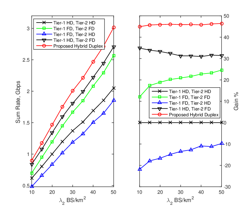
Fig. 8: Effectiveness of optimization with varied small cell density. The left figure shows the sum rate of users, and the right figure shows the gain over the conventional half-duplex HeNets.

According to [12], operating all BSs in full-duplex or half-duplex mode achieves higher throughput compared to the mixture of two mode BSs in each tier. Hence, we consider four duplex mode sets as benchmarks: 1) both tiers using half-duplex mode, 2) both tiers using full-duplex mode, 3) macro cells in full-duplex mode while small cells in half-duplex mode and 4) macro cells in half-duplex mode while small cells in full-duplex mode. Due to computational complexity, the exhaustive search results are omitted here. The sum rate obtained from different duplex mode sets are shown on the left of Fig. 8. We also show the gain of sum rate compared to the conventional half-duplex HetNets on the right. As observed in Fig. 8, our proposed hybrid-duplex mode outperforms all the benchmarks. As the density of small cells grows, the system performance of all the duplex mode sets improve. Higher density of BSs benefits the system performance in two aspects. First, the average load of BS decreases as the density grows, and the weights {ωm}\{\omega_{m}\} increase. Second, the average transmitting distance decreases as the BS density grows. However, a higher density of BSs causes stronger inter-cell interference, especially when small cells use full-duplex. It is the reason why the gain decreases in the case that macro cells use half-duplex and small cells use full-duplex in the right figure. On the other hand, the proposed algorithm shows a good balance between the duplex mode selection and interference suppression. The system gain stabilizes at about 45%45\% for all densities. It verifies that our algorithm can fulfill the potential of the proposed hybrid-duplex HetNets.

VI Conclusion

This paper proposes a novel received-power-based hybrid-duplex HetNet scheme. We characterize the SINR distribution and spectral efficiency by using stochastic geometry. Especially, inhomogeneous PPP model is used for both downlink and uplink analysis. A greedy algorithm for optimizing received power thresholds is also proposed. Extensive performance evaluations are conducted for both the analytical model and the optimization algorithm. The results show that the proposed hybrid-duplex HetNet scheme can improve the system performance significantly.

Appendix A

We consider a typical user in a two-tier HetNet. Define the following function:

f⁡(ξ)\displaystyle f\left(\xi\right) =12​log⁡(1+ξND)+12​log⁡(1+ϵ​ξNU)⏞Half-duplex\displaystyle=\overbrace{\frac{1}{2}\log\left(1+\frac{\xi}{N_{\text{D}}}\right)+\frac{1}{2}\log\left(1+\frac{\epsilon\xi}{N_{\text{U}}}\right)}^{\text{Half-duplex}}
−log⁡(1+ξR​S​ID+ND)−log⁡(1+ϵ​ξR​S​IU+NU)⏟Full-duplex,\displaystyle\underbrace{-\log\left(1+\frac{\xi}{RSI_{\text{D}}+N_{\text{D}}}\right)-\log\left(1+\frac{\epsilon\xi}{RSI_{\text{U}}+N_{\text{U}}}\right)}_{\text{Full-duplex}}, (73)

where ξ\xi is the average downlink received power. ϵ\epsilon is the user transmit power to the BS transmit power ratio. Note that the path losses are the same on both downlink and uplink channel. NDN_{\text{D}} and NUN_{\text{U}} are denoted as the sum of interference and noise on the downlink and uplink channel. R​S​IDRSI_{\text{D}} and R​S​IURSI_{\text{U}} are the residual self-interference of the user and its serving BS, respectively.

Eqn. (73) is the difference of data rate between the half-duplex mode and the full-duplex mode. When f⁡(ξ)≤0f\left(\xi\right)\leq 0, it means that the user has better performance in full-duplex mode. Otherwise, half-duplex mode is the better choice when f⁡(ξ)>0f\left(\xi\right)>0.

When R​S​ID≥NDRSI_{\text{D}}\geq N_{\text{D}} and R​S​IU≥NURSI_{\text{U}}\geq N_{\text{U}}, it is easy to have the following properties about f⁡(ξ)f\left(\xi\right) :

  1. 1)

    f⁡(0)=0f\left(0\right)=0;

  2. 2)

    when ξ\xi is sufficient small (but greater than 00), the gradient d​f​(ξ)d​ξ>0\frac{df(\xi)}{d\xi}>0;

  3. 3)

    when ξ>max⁡{R​S​ID−ND,1ϵ​(R​S​IU−NU)}\xi>\max\{RSI_{\text{D}}-N_{\text{D}},\frac{1}{\epsilon}\left(RSI_{\text{U}}-N_{\text{U}}\right)\}, the gradient d​f​(ξ)d​ξ<0\frac{df(\xi)}{d\xi}<0;

  4. 4)

    limξ→∞f⁡(ξ)<0\lim\limits_{\xi\to\infty}f\left(\xi\right)<0.

Hence, when SIC is not perfect and RSIs are relatively strong, a user suffering low received signal power (ξ\xi is sufficient small) should be scheduled as a half-duplex user (f⁡(ξ)>0f\left(\xi\right)>0). Otherwise, the user should be scheduled as a full-duplex user (f⁡(ξ)<0f\left(\xi\right)<0) when the received signal power is sufficient large. This is the reason why we consider a hybrid-duplex scheme based on average downlink received signal power.

Appendix B

According to the user association policy (2), the probability that the typical user is a full-duplex user in tier kk is

𝒜kFD=ℙ⁡(Dk≤Dk¯​(PkPk¯)1/α∩Dk≤δk)\displaystyle\mathcal{A}_{k}^{\text{FD}}=\mathbb{P}\left(D_{k}\leq D_{\bar{k}}\left(\frac{P_{k}}{P_{\bar{k}}}\right)^{1/\alpha}\cap D_{k}\leq\delta_{k}\right)
=1−∫0μk​(δk)ℙ⁡(Dk>r​(PkPk¯)1/α)​fDk¯​(r)​𝑑r\displaystyle=1-\int\limits_{0}^{\mu_{k}(\delta_{k})}\mathbb{P}\left(D_{k}>r\left(\frac{P_{k}}{P_{\bar{k}}}\right)^{1/\alpha}\right)f_{D_{\bar{k}}}(r)dr
−∫μk​(δk)∞ℙ(Dk>δk)fDk¯(r)dr,\displaystyle\qquad\qquad-\int\limits_{\mu_{k}(\delta_{k})}^{\infty}\mathbb{P}\left(D_{k}>\delta_{k}\right)f_{D_{\bar{k}}}(r)dr, (74)

where δk≜(Pkγk)1/α\delta_{k}\triangleq\left(\frac{P_{k}}{\gamma_{k}}\right)^{1/\alpha} and μk​(x)≜x​(Pk¯Pk)1/α\mu_{k}(x)\triangleq x\left(\frac{P_{\bar{k}}}{P_{k}}\right)^{1/\alpha}.

Using the property of PPP [19], we have the full-duplex association probability (16). Following a similar process, the half-duplex association probability (17) is derived. And (18) follows by the definition.

Appendix C

Take the point process of interfering full-duplex BSs ΦtFD\Phi_{t}^{\text{FD}} as example.

Refer to caption
Fig. 9: An instance of the distances between nodes.

As shown in Fig. 9, rr denotes as the distance between the typical user and the tagged BS. yy is the distance from the interfering BS to the typical user. Let ζ\zeta be the distance between the interfering BS and the handover point. According to the association policy, we have

ζ=r+ymax⁡{(PkPt)1/α−1,0}.\zeta=\frac{r+y}{\max\{(\frac{P_{k}}{P_{t}})^{1/\alpha}-1,0\}}. (75)

We assume that the coverage area of the interfering BS is a circular region around it with radius ζ\zeta. Then, the probability that there is user located in the coverage area, i.e. the probability that the interfering BS is active, can be expressed as 1−exp⁡(−λu​π​ζ2)1-\exp\left(-\lambda_{u}\pi\zeta^{2}\right). Thus the intensity measure function (19) is obtained. The process of deriving (20) is similar except that the interfering BS is scheduling a half-duplex user, which means that ζ\zeta should be greater than δt\delta_{t}. Intensity functions (21) and (22) follow the discussion in [14].

It is worth mentioning that all the intensity measure functions in this paper are the upper bound on accurate inhomogeneous intensities. Hence, the theoretical SINR distributions are lower-bounds, which is verified in Section V.

Appendix D

Take the downlink full-duplex SINR distribution 𝒞k1​,FD,D\mathcal{C}_{k}^{1\text{,FD,D}} as example.

𝒞k1​,FD,D​(T)=∫0∞ℙ⁡(θk1​,FD,D​(r)>T|DkFD=r)​fDkFD​(r)​𝑑r.\displaystyle\mathcal{C}_{k}^{1\text{,FD,D}}(T)=\int\limits_{0}^{\infty}\mathbb{P}(\theta_{k}^{1\text{,FD,D}}(r)>T|D_{k}^{\text{FD}}=r)f_{D_{k}^{\text{FD}}}(r)dr. (76)

According to the association policy (2), the cumulative density function (CDF) of the distance DkFDD_{k}^{\text{FD}} is:

ℙ⁡(DkFD≤x)={1,x>δk,ℙ⁡(Dk≤x|u∈𝒰kFD),x≤δk,\mathbb{P}(D_{k}^{\text{FD}}\leq x)=\begin{cases}1,x>\delta_{k},\\ \mathbb{P}(D_{k}\leq x|u\in\mathcal{U}_{k}^{\text{FD}}),x\leq\delta_{k},\end{cases} (77)

where

ℙ⁡(Dk≤x|u∈𝒰kFD)=ℙ⁡(Dk≤x,u∈𝒰kFD)ℙ⁡(u∈𝒰kFD)\displaystyle\mathbb{P}(D_{k}\leq x|u\in\mathcal{U}_{k}^{\text{FD}})=\frac{\mathbb{P}(D_{k}\leq x,u\in\mathcal{U}_{k}^{\text{FD}})}{\mathbb{P}(u\in\mathcal{U}_{k}^{\text{FD}})}
=1𝒜kFD[1−exp(−πλkx2−πλk¯(μk(x))2)\displaystyle=\frac{1}{\mathcal{A}_{k}^{\text{FD}}}\bigg[1-\exp\left(-\pi\lambda_{k}x^{2}-\pi\lambda_{\bar{k}}(\mu_{k}(x))^{2}\right)
−2πλk¯∫0μk​(x)rexp(−πλk(PkPk¯)2αr2−πλk¯r2)dr].\displaystyle\qquad-2\pi\lambda_{\bar{k}}\int\limits_{0}^{\mu_{k}(x)}r\exp\left(-\pi\lambda_{k}\Big(\frac{P_{k}}{P_{\bar{k}}}\Big)^{\frac{2}{\alpha}}r^{2}-\pi\lambda_{\bar{k}}r^{2}\right)dr\bigg].

Thus the probability density function (pdf) is:

fDkFD​(x)={0,x>δk,2​π​λk𝒜kFD​[x​exp⁡(−π​λk​x2−π​λk¯​(μk​(x))2)],x≤δk.\displaystyle f_{D_{k}^{\text{FD}}}(x)=\begin{cases}0,x>\delta_{k},\\ \frac{2\pi\lambda_{k}}{\mathcal{A}_{k}^{\text{FD}}}\left[x\exp\left(-\pi\lambda_{k}x^{2}-\pi\lambda_{\bar{k}}(\mu_{k}(x))^{2}\right)\right],x\leq\delta_{k}.\end{cases} (78)

The conditional SINR distribution on channel 11 of a full-duplex user at distance rr from its serving BS is

ℙ⁡(θk1​,FD,D>T|DkFD=r)\displaystyle\mathbb{P}\left(\theta_{k}^{1\text{,FD,D}}>T|D_{k}^{\text{FD}}=r\right)
=exp⁡(−TS​S​I​N​Rk,u​(r))​∏t=k,k¯𝔼It,k1​,D​[exp⁡(−T​rαPk​It,k1​,D)],\displaystyle=\exp\left(-\frac{T}{SSINR_{k,u}(r)}\right)\prod\limits_{t=k,\bar{k}}\mathbb{E}_{I_{t,k}^{1\text{,D}}}\left[\exp\left(-\frac{Tr^{\alpha}}{P_{k}}I_{t,k}^{1\text{,D}}\right)\right], (79)

Using the interference expression (6), we have

𝔼It,k1​,D​[exp⁡(−T​rαPk​It,k1​,D)]\displaystyle\mathbb{E}_{I_{t,k}^{1\text{,D}}}\left[\exp\left(-\frac{Tr^{\alpha}}{P_{k}}I_{t,k}^{1\text{,D}}\right)\right]
=(a)​ℒΦtFD​(r,T)​ℒΦu,tFD​(r,T)​ℒΦtHD​(r,T),\displaystyle\qquad\qquad\overset{(a)}{=}\mathcal{L}_{\Phi_{t}^{\text{FD}}}(r,T)\mathcal{L}_{\Phi_{u,t}^{\text{FD}}}(r,T)\mathcal{L}_{\Phi_{t}^{\text{HD}}}(r,T), (80)

where (a)(a) follows that ΦtFD\Phi_{t}^{\text{FD}}, Φu,tFD\Phi_{u,t}^{\text{FD}} and ΦtHD\Phi_{t}^{\text{HD}} are assumed to be mutually independent, hbi,u0h_{b_{i},u_{0}} and hubi,u0h_{u_{b_{i}},u_{0}} are i.i.d. (hi,j∼exp⁡(1)h_{i,j}\sim\exp(1)). Using the probability generating functional (PGFL) [21] of PPP and the Laplace transform ℒh​(s)=11+s\mathcal{L}_{h}(s)=\frac{1}{1+s} of h∼exp⁡(1)h\sim\exp(1), we have (28) and (29). Δk,t​(r)=(PtPk)1/α​r\Delta_{k,t}(r)=\left(\frac{P_{t}}{P_{k}}\right)^{1/\alpha}r is the lower-bound of the distance to the interfering BS in tier tt when the typical user is in tier kk.

The derivation of (30) is similar except the interesting lower-bound max⁡{r​(PtPk)1/α−δt,0}\max\{r(\frac{P_{t}}{P_{k}})^{1/\alpha}-\delta_{t},0\}. Let ζ\zeta be the distance between the interfering full-duplex user and its serving BS. Remind that rr is the distance between the typical user and the tagged BS, and yy denotes as the distance from the interfering user to the typical one. There are two critical conditions: (i) the interfering user is full-duplex; (ii) the typical user is served by the tagged BS. Hence we have

{ζ≤δtPk​r−α≥Pt​(y+ζ)−α⇒y≥r​(PtPk)1/α−δt,\displaystyle\begin{cases}\zeta\leq\delta_{t}\\ P_{k}r^{-\alpha}\geq P_{t}(y+\zeta)^{-\alpha}\end{cases}\Rightarrow y\geq r(\frac{P_{t}}{P_{k}})^{1/\alpha}-\delta_{t}, (81)

and then (30) is obtained.

The lower-bound max⁡{δt​(PkPt)1/α−r,0}\max\{\delta_{t}(\frac{P_{k}}{P_{t}})^{1/\alpha}-r,0\} in (31) is obtained considering two different conditions: (i) the interfering user is half-duplex; (ii) the interfering user is not served by the tagged BS. Hence we have

{ζ≥δtPk​(r+y)−α≤Pt​ζ−α⇒y≥δt​(PkPt)1/α−r.\displaystyle\begin{cases}\zeta\geq\delta_{t}\\ P_{k}(r+y)^{-\alpha}\leq P_{t}\zeta^{-\alpha}\end{cases}\Rightarrow y\geq\delta_{t}(\frac{P_{k}}{P_{t}})^{1/\alpha}-r. (82)

The proofs of (25) and (26) are omitted, which can be derived following a similar process.

Appendix E

The proof of the uplink SINR distributions is roughly the same as that of downlink. Similar to Appendix D, we can easily have

𝒞k1​,FD,U=∫0∞ℙ⁡(θk1​,FD,U​(r)>T|DkFD=r)​fDkFD​(r)​𝑑r,\displaystyle\mathcal{C}_{k}^{1\text{,FD,U}}=\int\limits_{0}^{\infty}\mathbb{P}\left(\theta_{k}^{1\text{,FD,U}}(r)>T|D_{k}^{\text{FD}}=r\right)f_{D_{k}^{\text{FD}}}(r)dr, (83)
ℙ⁡(θk1​,FD,U​(r)>T|DkFD=r)\displaystyle\mathbb{P}\left(\theta_{k}^{1\text{,FD,U}}(r)>T|D_{k}^{\text{FD}}=r\right)
=exp⁡(−TS​S​I​N​Ru,k)​∏t=k,k¯𝔼It,k1​,U​[exp⁡(−T​rαPu​It,k1​,U)].\displaystyle=\exp\left(-\frac{T}{SSINR_{u,k}}\right)\prod\limits_{t=k,\bar{k}}\mathbb{E}_{I_{t,k}^{1\text{,U}}}\left[\exp\left(-\frac{Tr^{\alpha}}{P_{u}}I_{t,k}^{1\text{,U}}\right)\right]. (84)

Using the interference expression (7), we have

𝔼It,k1​,U​[exp⁡(−T​rαPu​It,k1​,U)]=ℒΦtFD​(r,T)​ℒΦu,tFD​(r,T)​ℒΦtHD​(r,T),\displaystyle\mathbb{E}_{I_{t,k}^{1\text{,U}}}\Big[\exp(-\frac{Tr^{\alpha}}{P_{u}}I_{t,k}^{1\text{,U}})\Big]=\mathcal{L}_{\Phi_{t}^{\text{FD}}}(r,T)\mathcal{L}_{\Phi_{u,t}^{\text{FD}}}(r,T)\mathcal{L}_{\Phi_{t}^{\text{HD}}}(r,T), (85)

If the distance between the typical user and the tagged BS is rr, there is no interfering BS in the shadowed area as shown in Fig. 10 (a) on page 1313, considering the user association policy. However, the no-interfering-BS area is difficult to characterize. Hence, we make such an approximation that the no-interfering-BS area in Fig. 10 (a) is approximated to the shadowed sector in Fig. 10 (b). The sector has the same area as the shadowed circular area in the left figure. Thus we can have the interfering area ratio

pk,tI=1−π​(Δk,t​(r))2π​(Δk,t​(r)+r)2​=(a)​1−(Pt1/αPt1/α+Pk1/α)2.\displaystyle p_{k,t}^{I}=1-\frac{\pi(\Delta_{k,t}(r))^{2}}{\pi(\Delta_{k,t}(r)+r)^{2}}\overset{(a)}{=}1-\left(\frac{P_{t}^{1/\alpha}}{P_{t}^{1/\alpha}+P_{k}^{1/\alpha}}\right)^{2}. (86)

Hence we have (40) and (41).

Refer to caption
Fig. 10: The no-interfering-BS area and its approximation.

References

  • [1] A. Sabharwal, P. Schniter, D. Guo, D. Bliss, S. Rangarajan, and R. Wichman, “In-band full-duplex wireless: Challenges and opportunities,” IEEE Journal on Selected Areas in Communications, vol. 32, no. 9, pp. 1637–1652, Sep. 2014.
  • [2] S. Hong, J. Brand, J. Choi, M. Jain, J. Mehlman, S. Katti, and P. Levis, “Applications of self-interference cancellation in 5G and beyond,” IEEE Communications Magazine, vol. 52, no. 2, pp. 114–121, Feb. 2014.
  • [3] D. Bharadia, E. McMilin, and S. Katti, “Full duplex radios,” in ACM SIGCOMM 2013, New York, NY, USA, 2013, pp. 375–386.
  • [4] C. Teyan and S. Liu, “A multi-stage self-interference canceller for full-duplex wireless communications,” in 2015 IEEE Global Communications Conference (GLOBECOM), 2015.
  • [5] S. Goyal, P. Liu, S. Hua, and S. Panwar, “Analyzing a full-duplex cellular system,” in CISS 2013, Mar. 2013, pp. 1–6.
  • [6] M. Mohammadi, H. A. Suraweera, I. Krikidis, and C. Tellambura, “Full-duplex radio for uplink/downlink transmission with spatial randomness,” in Proc. IEEE ICC 2015.
  • [7] C. Psomas and I. Krikidis, “Outage analysis of full-duplex architectures in cellular networks,” in Proc. IEEE VTC 2015 Spring, Glasgow.
  • [8] S. Goyal, P. Liu, S. Panwar, R. Yang, R. A. DiFazio, and E. Bala, “Full duplex operation for small cells,” Dec. 2014. [Online]. Available: http://arxiv.org/abs/1412.8708
  • [9] J. Yao, S. Feng, X. Zhou, and Y. Liu, “Secure Routing in Multihop Wireless Ad-Hoc Networks With Decode-and-Forward Relaying,” IEEE Transactions on Communications, vol. 64, no. 2, pp. 753–764, 2016.
  • [10] H.-S. Jo, Y. J. Sang, P. Xia, and J. Andrews, “Heterogeneous cellular networks with flexible cell association: A comprehensive downlink sinr analysis,” IEEE Transactions on Wireless Communications, vol. 11, no. 10, pp. 3484–3495, 2012.
  • [11] W. Tang, S. Feng, Y. Liu, and M. C. Reed, “Joint low-power transmit and cell association in heterogeneous networks,” in 2015 IEEE Global Communications Conference (GLOBECOM), 2015, pp. 1–6.
  • [12] J. Lee and T. Quek, “Hybrid full-/half-duplex system analysis in heterogeneous wireless networks,” IEEE Transactions on Wireless Communications, vol. 14, no. 5, pp. 2883–2895, 2015.
  • [13] B. Błaszczyszyn and D. Yogeshwaran, “Clustering comparison of point processes, with applications to random geometric models,” in Stochastic Geometry, Spatial Statistics and Random Fields, ser. Lecture Notes in Mathematics, V. Schmidt, Ed. Springer International Publishing, 2015, no. 2120, pp. 31–71.
  • [14] S. Singh, X. Zhang, and J. G. Andrews, “Joint rate and SINR coverage analysis for decoupled uplink-downlink biased cell associations in HetNets,” IEEE Transactions on Wireless Communications, vol. 14, no. 10, pp. 5360–5373, 2015.
  • [15] F. J. Martin-Vega, G. Gomez, M. C. Aguayo-Torres, and M. Di Renzo, “Analytical modeling of interference aware power control for the uplink of heterogeneous cellular networks,” Jan. 2016. [Online]. Available: http://arxiv.org/abs/1601.03164
  • [16] Y. Lin, W. Bao, W. Yu, and B. Liang, “Optimizing user association and spectrum allocation in hetnets: A utility perspective,” IEEE Journal on Selected Areas in Communications, vol. 33, no. 6, pp. 1025–1039, Jun. 2015.
  • [17] B. Blaszczyszyn, M. Karray, and H. Keeler, “Using Poisson processes to model lattice cellular networks,” in 2013 Proceedings IEEE INFOCOM, Apr. 2013, pp. 773–781.
  • [18] 3GPP, “Evolved universal terrestrial radio access (E-UTRA); user equipment (UE) procedures in idle mode,” TS 36.304 version 11.6.0 Release 11, Jan. 2014.
  • [19] F. Baccelli, “Stochastic geometry and wireless networks: Volume I theory,” Foundations and Trends® in Networking, vol. 3, no. 3-4, pp. 249–449, 2009.
  • [20] D. Ramirez and B. Aazhang, “Optimal routing and power allocation for wireless networks with imperfect full-duplex nodes,” IEEE Transactions on Wireless Communications, vol. 12, no. 9, pp. 4692–4704, Sep. 2013.
  • [21] D. Stoyan, W. S. Kendall, and J. Mecke, Stochastic geometry and its applications, 3rd ed. John Wiley & Sons Inc, 2013.