跳到论文正文
W Papers独立论文阅读器 arXiv:1608.05968 论文正文 计算阅读时间 · 0%
引用这篇论文根据当前论文元数据生成,正式投稿前建议核对。


License: arXiv.org perpetual non-exclusive license
arXiv:1608.05968v2 [cond-mat.mes-hall] 21 Oct 2016

Coulomb-blockade effect in nonlinear mesoscopic capacitors

M. I. Alomar Affiliation: Institut de Física Interdisciplinària i Sistemes Complexos IFISC (CSIC-UIB), E-07122 Palma de Mallorca, Spain Affiliation: Departament de Física, Universitat de les Illes Balears, E-07122 Palma de Mallorca, Spain    Jong Soo Lim Affiliation: School of Physics, Korea Institute for Advanced Study, Seoul 130-722, Korea    David Sánchez Affiliation: Institut de Física Interdisciplinària i Sistemes Complexos IFISC (CSIC-UIB), E-07122 Palma de Mallorca, Spain Affiliation: Departament de Física, Universitat de les Illes Balears, E-07122 Palma de Mallorca, Spain
Abstract

We consider an interacting quantum dot working as a coherent source of single electrons. The dot is tunnel coupled to a reservoir and capacitively coupled to a gate terminal with an applied ac potential. At low frequencies, this is the quantum analog of the R​CRC circuit with a purely dynamical response. We investigate the quantized dynamics as a consequence of ac pulses with large amplitude. Within a Keldysh-Green function formalism we derive the time dependent current in the Coulomb blockade regime. Our theory thus extends previous models that considered either noninteracting electrons in nonlinear response or interacting electrons in the linear regime. We prove that the electron emission and absorption resonances undergo a splitting when the charging energy is larger than the tunnel broadening. For very large charging energies, the additional peaks collapse and the original resonances are recovered, though with a reduced amplitude. Quantization of the charge emitted by the capacitor is reduced due to Coulomb repulsion and additional plateaus arise. Additionally, we discuss the differential capacitance and resistance as a function of time. We find that to leading order in driving frequency the current can be expressed as a weighted sum of noninteracting currents shifted by the charging energy.

pacs
73.23.-b, 73.23.Hk, 73.63.Kv

I Introduction

Real-time manipulation of electrons is one of the greatest achievements in modern nanoelectronics [1, 2, 3]. The characteristic setup comprises a submicron-sized cavity or quantum dot tunnel coupled to a reservoir through a quantum point contact. Then, a time dependent driving voltage is applied to a electrostatically coupled metallic gate placed on top of the dot. As a consequence, dc transport is impossible and the system response is purely dynamical. The low-frequency admittance measured with cryogenic low-noise amplifiers can be understood from the serial combination of a charge relaxation resistance and a quantum capacitance [4, 5]. It turns out that in the linear regime (small ac amplitudes) the charge relaxation resistance is quantized for a single spin-polarized channel [6], a theoretical prediction that was experimentally confirmed [1]. For drivings with larger amplitudes (nonlinear regime), the system works as an on-demand single-electron source [2], in analogy with single-photon sources [7, 8], with alternate sequences of electron emission and absorption during a driving period in the fast (GHz) regime. When the voltage pulse has a Lorentzian shape [9, 10, 11, 12], recent progress has shown that the holes can be efficiently removed from the stream of excitations when the pulse is applied to an Ohmic contact [13]. These phenomena imply the observation of quantized currents ensured by charge quantization, which might be useful in metrology applications [14] and quantum computation designs [15, 16, 17].

Now, tunneling electrons feel repulsive interactions that yield Coulomb blockade, a prominent effect in small-capacitance conductors which manifests itself as an increased resistance of a quantum dot junction at finite bias voltages [18]. In fact, the effect is quite ubiquitous in nanoscale systems and arises not only in quantum dots but also in carbon nanotubes [19], molecular transistors [20], and optical lattices [21]. Therefore, it is natural to investigate the role of Coulomb blockade effects in single-electron sources. This is the goal we want to accomplish in this work. We begin by noticing that electron-electron interactions have been widely analyzed in the quantum R​CRC circuit [22, 23, 24, 25, 26, 27, 28, 29, 30, 31, 32, 33, 34, 35, 36, 37, 38, 39]. However, these works have mostly focused on the linear regime (for an exception, see Ref. [35]). The nonlinear regime is interesting because both the capacitance and the charge relaxation resistance acquire an explicit time dependence [40]. This result was found for noninteracting electrons. Here, we give full expressions for the capacitive and the dissipative parts of the current valid in the case of strong interactions that lead to Coulomb blockade effect. We predict that this effect should be visible as a splitting of the dynamical current peaks for both emitted and absorbed electrons. Importantly, the simultaneous emission of pairs of electrons in the non-interacting case is modified to a subsequent emission of two electrons.
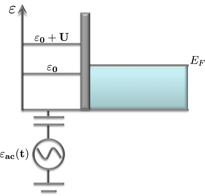
Refer to caption
Figure 1: Schematic representation of a single-electron source comprising a single-level quantum dot coupled capacitively to an ac oscillating signal, εa​c​(t)\varepsilon_{ac}(t). The dot can exchange electrons with an attached reservoir (Fermi energy EFE_{F}) via a tunnel barrier. The dot energy level is denoted with ε0\varepsilon_{0} and Coulomb repulsion is given by the charging energy UU.

The energy diagram of our system is sketched in Fig. 1. We consider a single-level quantum dot (energy ε0\varepsilon_{0}) coupled to a Fermi sea of electrons (Fermi energy EFE_{F}). The coupling region between the dot and the reservoir is typically a pinched-off quantum point contact that we depict in Fig. 1 with a tunnel barrier. This part represents the resistive component of the quantum circuit, through which electrons can hop on and off the dot. The position of ε0\varepsilon_{0} can be tuned with a dc gate potential applied to the point contact [2] (not shown in Fig. 1). Additionally, the dot is coupled to a nearby gate terminal with an externally applied harmonic potential εa​c​(t)\varepsilon_{ac}(t). This is the capacitive part of the R​CRC circuit. Finally, a charging energy UU is required to charge the dot with two electrons having opposite spins. The situation considered in this paper is experimentally relevant for small dots. The case of large dots with many quantum levels was treated in Ref. [22], where a Hartree-Fock approximation was employed to account for Coulomb interactions and screening effects. Here, we consider the Anderson model with a single level and a constant interaction energy. This model has been successfully applied to the Fermi liquid limit connected to the Korringa-Shiba relation [31], unveiling strong departures of the charge relaxation resistance from universality [32].

II Model Hamiltonian and Keldysh-Green function formalism

Our theoretical discussion starts with the Anderson Hamiltonian of a mesoscopic capacitor, H=HR+HT+HDH=H_{R}+H_{T}+H_{D}, where HRH_{R} describes the single reservoir, HTH_{T} is the tunnel coupling between the reservoir and the quantum dot (QD) and HDH_{D} models the QD:

HR\displaystyle H_{R} =\displaystyle= ∑k​σεk​ck​σ†​ck​σ,\displaystyle\sum_{k\sigma}\varepsilon_{k}c_{k\sigma}^{\dagger}c_{k\sigma}\,, (1a)
HT\displaystyle H_{T} =\displaystyle= ∑k​σ(Vk∗​dσ†​ck​σ+Vk​ck​σ†​dσ),\displaystyle\sum_{k\sigma}\left(V_{k}^{\ast}d_{\sigma}^{\dagger}c_{k\sigma}+V_{k}c_{k\sigma}^{\dagger}d_{\sigma}\right)\,, (1b)
HD\displaystyle H_{D} =\displaystyle= ∑σεσ​(t)​dσ†​dσ+U​n↑​n↓,\displaystyle\sum_{\sigma}\varepsilon_{\sigma}(t)d_{\sigma}^{\dagger}d_{\sigma}+Un_{\uparrow}n_{\downarrow}\,, (1c)

with nσ=dσ†​dσn_{\sigma}=d_{\sigma}^{\dagger}d_{\sigma} the occupation number operator and εσ​(t)=εσ+εa​c​(t)\varepsilon_{\sigma}(t)=\varepsilon_{\sigma}+\varepsilon_{ac}(t) including both the QD energy level, εσ=ε0+σ​ΔZ/2\varepsilon_{\sigma}=\varepsilon_{0}+\sigma\Delta_{Z}/2 (here ΔZ\Delta_{Z} denotes the Zeeman splitting due to interaction with an external magnetic field), and the oscillating potential applied to the gate, εa​c​(t)=εa​c​cos⁡Ω​t\varepsilon_{ac}(t)=\varepsilon_{ac}\cos\Omega t, where εa​c\varepsilon_{ac} is the ac amplitude and Ω\Omega is the driving frequency. We emphasize that ε0\varepsilon_{0} and εa​c​(t)\varepsilon_{ac}(t) can be tuned independently, as experimentally demonstrated [2], with a dc and ac voltage, respectively, applied to the quantum point contact and the gate electrode: ε0=−e​VQPC\varepsilon_{0}=-eV_{\rm QPC} and εa​c=−e​Vg\varepsilon_{ac}=-eV_{g}. This allows us to treat the position of the QD level relative to the Fermi energy and the ac amplitude as separate parameters in our calculations. The sinusoidal drive considered here is convenient because the derivative of the drive is proportional to the frequency and thus easily Fourier decomposed. Different drives such as a step function do not shows this nice property and add mathematical difficulties to the formalism. Hence, we restrict ourselves to the monochromatic case.

In the Hamiltonian HH, σ\sigma labels the electron spin and hereafter we consider the nonmagnetic case (ΔZ=0\Delta_{Z}=0). However, the magnetic (ΔZ≠0\Delta_{Z}\neq 0) situation can be easily included in our model but we focus on the spin-degenerate case. This is an important difference with the samples of Refs. [1, 2], which operate in the quantum Hall regime to achieve single-channel propagation with no spin degeneracy.

In Eq. (1a), εk\varepsilon_{k} represents the reservoir energy dispersion with momentum kk and ck​σ†​(ck​σ)c_{k\sigma}^{\dagger}(c_{k\sigma}) creates (annihilates) a conduction band electron. The tunnel hamiltonian given by Eq. (1b) contains the tunnel amplitude VkV_{k} and the fermionic operator dσ†​(dσ)d_{\sigma}^{\dagger}(d_{\sigma}), which creates (annihilates) a localized electron in the dot. Finally, U=e2/(Cg+CR)U=e^{2}/(C_{g}+C_{R}) in Eq. (1c) is the charging energy, which we also take as a tunable parameter depending on the capacitive strengths with the coupled gate, CgC_{g}, and eventually with the reservoir, CRC_{R}.

The time dependent field εa​c​(t)\varepsilon_{ac}(t) induces a purely dynamical charge current IR​(t)I_{R}(t) that can be measured at the reservoir. Since HH commutes with the total charge, IRI_{R} is determined from the change rate of the dot occupation, I⁡(t)I(t):

IR​(t)+I⁡(t)=0,I_{R}(t)+I(t)=0\,, (2)

where I⁡(t)=e​∂t∑σ⟨dσ†​dσ⟩​(t)I(t)=e\partial_{t}\sum_{\sigma}\langle d_{\sigma}^{\dagger}d_{\sigma}\rangle(t) and IR​(t)=e​∂t∑k,σ⟨ck​σ†​ck​σ⟩​(t)I_{R}(t)=e\partial_{t}\sum_{k,\sigma}\langle c_{k\sigma}^{\dagger}c_{k\sigma}\rangle(t) with ee the unit of charge. Here, ∂t\partial_{t} denotes the time derivative. Equation (2) thus represents the electronic charge conservation. In what follows, we focus on I⁡(t)I(t) because it can be directly expressed in terms of the QD Green’s function without further manipulation, as shown below. The physical current IRI_{R} (since it amounts to a flux) can then be obtained immediately from Eq. (2).

Let Gσ<​(t,t′)=i⁡⟨dσ†​(t′)​dσ​(t)⟩G_{\sigma}^{<}(t,t^{\prime})=i\langle d_{\sigma}^{\dagger}(t^{\prime})d_{\sigma}(t)\rangle be the lesser Green’s function [41, 42] for the dot operators. Clearly, the QD occupation ⟨nσ​(t)⟩=⟨dσ†​(t)​dσ​(t)⟩\langle n_{\sigma}(t)\rangle=\langle d_{\sigma}^{\dagger}(t)d_{\sigma}(t)\rangle can be written in terms of the lesser Green’s function. The current is hence calculated as

I⁡(t)\displaystyle I(t) =e​∂t∑σ⟨nσ​(t)⟩=e​∂t∑σ(−i​Gσ<​(t,t))\displaystyle=e\partial_{t}\sum_{\sigma}\left\langle n_{\sigma}(t)\right\rangle=e\partial_{t}\sum_{\sigma}\Big(-i{G}_{\sigma}^{<}(t,t)\Big)
=e​∂t∑σ∫d​ε2​π​i​Gσ<​(t,ε),\displaystyle=e\partial_{t}\sum_{\sigma}\int\frac{d\varepsilon}{2\pi i}{G}_{\sigma}^{<}(t,\varepsilon)\,, (3)

where in the last line we express the lesser dot Green’s function in a mixed time energy notation [43, 44]. This representation is especially useful for nonstationary scattering problems in the adiabatic limit [45, 46]. Its connection with the original double time picture and the corresponding Fourier transform is discussed in Appendix A.

Our regime of interest here is the adiabatic case (small frequency Ω\Omega) but arbitrary values of the ac amplitude εa​c\varepsilon_{ac}. In that case, the Green’s function is expected to display small deviations around a frozen state in time characterized by a stationary scattering matrix with time dependent parameters. This approximation is good when ℏ​Ω\hbar\Omega is the smallest energy scale of our problem. For a prototypical R​CRC circuit [1], ℏ​Ω≃0.2\hbar\Omega\simeq 0.2 μ\mueV, which is at least fifty times smaller than the tunnel coupling Γ≃10\Gamma\simeq 10 μ\mueV. Therefore, the electron interacts only weakly with the ac potential before tunneling into or out of the QD. The frequency expansion reads,

Gσ<​(t,ε)=Gσ<,f​(t,ε)+ℏ​Ω​Gσ<,(1)​(t,ε)+O⁡(Ω2),\displaystyle{G}_{\sigma}^{<}(t,\varepsilon)={G}_{\sigma}^{<,f}(t,\varepsilon)+\hbar\Omega{G}_{\sigma}^{<,(1)}(t,\varepsilon)+{O}(\Omega^{2})\,, (4)

where the superscript ff denotes the frozen approximation and (1)(1) implies the first order in driving frequency Ω\Omega. Second-order terms and beyond are neglected, which suffices for the purposes of this work. (Inductive-like effects have been studied in Ref. [47]). We stress that the zeroth-order (frozen) term in Ω\Omega is still time dependent. No assumption has been made on the strength of the amplitude, which can be arbitrarily large, driving the system into the nonlinear regime.

Substituting Eq. (4) into Eq. (3), we find similar expansions for the occupation and the current,

I⁡(t)\displaystyle I(t) ≃e​∂t∑σ∫d​ε2​π​i​(Gσ<,f​(t,ε)+ℏ​Ω​Gσ<,(1)​(t,ε))\displaystyle\simeq e\partial_{t}\sum_{\sigma}\int\frac{d\varepsilon}{2\pi i}\Big({G}_{\sigma}^{<,f}(t,\varepsilon)+\hbar\Omega{G}_{\sigma}^{<,(1)}(t,\varepsilon)\Big)
=e​∂t∑σ(⟨nσ​(t)⟩f+⟨nσ​(t)⟩(1))\displaystyle=e\partial_{t}\sum_{\sigma}(\left\langle n_{\sigma}(t)\right\rangle^{f}+\left\langle n_{\sigma}(t)\right\rangle^{(1)})
=I(1)​(t)+I(2)​(t).\displaystyle=I^{(1)}(t)+I^{(2)}(t)\,. (5)

From the definition given by Eq. (3), it follows that the leading order for the current is first order in Ω\Omega. To be consistent, we therefore keep the current terms in Eq. (5) up to second order in Ω\Omega. The physical implication says that I(1)I^{(1)} represents a capacitive-like contribution while I(2)I^{(2)} is understood as a dissipative component [40].

This interpretation can be substantiated by introducing a quantum R​CRC circuit model (a capacitor and a resistor in a series with an applied ac potential) with time dependent capacitance and resistance functions,

eI(t)≃−C∂(t)∂tεa​c(t)+R∂(t)C∂(t)∂t(C∂(t)∂tεa​c(t)).eI(t)\simeq-C_{\partial}(t)\partial_{t}\varepsilon_{ac}(t)\\ +R_{\partial}(t)C_{\partial}(t)\partial_{t}(C_{\partial}(t)\partial_{t}\varepsilon_{ac}(t))\,. (6)

This relation is valid at low frequency for both the linear and the nonlinear regimes. In Eq. (6) C∂​(t)C_{\partial}(t) is the differential capacitance and R∂​(t)R_{\partial}(t) the differential resistance. Both depend on time because they constitute a generalization of the linear-response quantum capacitance CqC_{q} and charge relaxation resistance RqR_{q} [4] to the nonlinear ac transport regime [40]. Combining Eq. (5) with Eq. (6), we can find expressions for C∂​(t)C_{\partial}(t) and R∂​(t)R_{\partial}(t). Therefore, our goal is first to obtain an equation for Gσ<​(t,ε)G^{<}_{\sigma}(t,\varepsilon) in the presence of Coulomb interactions and oscillating voltages.

III Equation of motion

The temporal evolution of the dot Green’s function is determined from the commutator of dσd_{\sigma} with HH (Heisenberg equation of motion). It is convenient to consider the time-ordered Green’s function Gσ​(t,t′)≡⟨⟨dσ,dσ†⟩⟩​(t,t′)=−i⁡⟨𝒯​dσ​(t)​dσ†​(t′)⟩G_{\sigma}(t,t^{\prime})\equiv\langle\langle d_{\sigma},d_{\sigma}^{\dagger}\rangle\rangle(t,t^{\prime})=-i\langle{\cal{T}}d_{\sigma}(t)d_{\sigma}^{\dagger}(t^{\prime})\rangle. After some straightforward steps, we find that the time-ordered Green’s function satisfies the integral (Dyson) equation

Gσ​(t,t′)=gσ​(t,t′)+∫d​sℏ​Gσ​(t,s)​εa​c​(s)​gσ​(s,t′)+∫d​sℏ∫d​s′ℏGσ(t,s′)Σ0(s′,s)gσ(s,t′)+U∫d​sℏ⟨⟨dσ,dσ†nσ¯⟩⟩(t,s)gσ(s,t′),G_{\sigma}(t,t^{\prime})=\text{g}_{\sigma}(t,t^{\prime})+\int\frac{ds}{\hbar}~G_{\sigma}(t,s)\varepsilon_{ac}(s)\text{g}_{\sigma}(s,t^{\prime})\\ +\int\frac{ds}{\hbar}~\int\frac{ds^{\prime}}{\hbar}~G_{\sigma}(t,s^{\prime})\Sigma_{0}(s^{\prime},s)\text{g}_{\sigma}(s,t^{\prime})\\ +U\int\frac{ds}{\hbar}~\langle\langle d_{\sigma},d_{\sigma}^{\dagger}n_{\bar{\sigma}}\rangle\rangle(t,s)\text{g}_{\sigma}(s,t^{\prime})\,, (7)

where σ¯=−σ\bar{\sigma}=-\sigma. Σ0​(t,t′)=∑k|Vk|2​gk​(t,t′)\Sigma_{0}(t,t^{\prime})=\sum_{k}|V_{k}|^{2}\text{g}_{k}(t,t^{\prime}) is the tunnel self-energy with gk⁡(σ)​(t,t′)\text{g}_{k(\sigma)}(t,t^{\prime}) the isolated reservoir (dot) Green’s function in the absence of the ac driving potential. The retarded/advanced and lesser Green’s functions can then be obtained from the Langreth’s analytic continuation rules [42].

To consider the effect of UU, we now generate an additional integral equation for the correlator ⟨⟨dσ,dσ†​nσ¯⟩⟩​(t,t′)\langle\langle d_{\sigma},d_{\sigma}^{\dagger}n_{\bar{\sigma}}\rangle\rangle(t,t^{\prime}) in Eq. (7):

⟨⟨dσ,dσ†​nσ¯⟩⟩​(t,t′)=⟨nσ¯​(t)⟩​gσ​(t,t′)+∫d​sℏ⟨⟨dσ,dσ†nσ¯⟩⟩(t,s)εa​c(s)gσ(s,t′)+∑k∫d​sℏ(Vk⟨⟨dσ,c†k​σnσ¯⟩⟩(t,s)+Vk​⟨⟨dσ,dσ†​ck​σ¯​dσ¯⟩⟩​(t,s)OPEN−Vk∗​⟨⟨dσ,dσ†​dσ¯†​ck​σ¯⟩⟩​(t,s))​gσ​(s,t′)+U∫d​sℏ⟨⟨dσ,dσ†nσ¯⟩⟩(t,s)gσ(s,t′),\langle\langle d_{\sigma},d_{\sigma}^{\dagger}n_{\bar{\sigma}}\rangle\rangle(t,t^{\prime})=\left\langle n_{\bar{\sigma}}(t)\right\rangle\text{g}_{\sigma}(t,t^{\prime})\\ +\int\frac{ds}{\hbar}~\langle\langle d_{\sigma},d_{\sigma}^{\dagger}n_{\bar{\sigma}}\rangle\rangle(t,s)\varepsilon_{ac}(s)\text{g}_{\sigma}(s,t^{\prime})\\ +\sum_{k}\int\frac{ds}{\hbar}~\left(V_{k}\langle\langle d_{\sigma},c^{\dagger}_{k\sigma}n_{\bar{\sigma}}\rangle\rangle(t,s)\right.\\ \left.+V_{k}\langle\langle d_{\sigma},d_{\sigma}^{\dagger}c_{k\bar{\sigma}}d_{\bar{\sigma}}\rangle\rangle(t,s)\right.\\ \left.-V_{k}^{\ast}\langle\langle d_{\sigma},d_{\sigma}^{\dagger}d_{\bar{\sigma}}^{\dagger}c_{k\bar{\sigma}}\rangle\rangle(t,s)\right)\text{g}_{\sigma}(s,t^{\prime})\\ +\,U\int\frac{ds}{\hbar}~\langle\langle d_{\sigma},d_{\sigma}^{\dagger}n_{\bar{\sigma}}\rangle\rangle(t,s)\text{g}_{\sigma}(s,t^{\prime})\,, (8)

where three new correlation functions arise. Since we are interested in the Coulomb blockade regime, we can neglect charge and spin excitations. This truncated equation of motion approach is good in the weak tunneling regime or for not very low temperatures, in which case Kondo correlations can be disregarded [48]. As a consequence, we neglect the spin-flip correlators in Eq. (8):

⟨⟨dσ,dσ†​dσ¯†​ck​σ¯⟩⟩​(t,s)≃0,\displaystyle\langle\langle d_{\sigma},d_{\sigma}^{\dagger}d_{\bar{\sigma}}^{\dagger}c_{k\bar{\sigma}}\rangle\rangle(t,s)\simeq 0\,, (9a)
⟨⟨dσ,dσ†​ck​σ¯​dσ¯⟩⟩​(t,s)≃0.\displaystyle\langle\langle d_{\sigma},d_{\sigma}^{\dagger}c_{k\bar{\sigma}}d_{\bar{\sigma}}\rangle\rangle(t,s)\simeq 0\,. (9b)

Next, we calculate the equation of motion for ⟨⟨dσ,ck​σ†​nσ¯⟩⟩​(t,t′)\langle\langle d_{\sigma},c^{\dagger}_{k\sigma}n_{\bar{\sigma}}\rangle\rangle(t,t^{\prime}):

⟨⟨dσ,ck​σ†​nσ¯⟩⟩​(t,t′)=∫d​sℏ​Vk∗​⟨⟨dσ,dσ†​nσ¯⟩⟩​(t,s)​gk​(s,t′)+∑k∫d​sℏ(Vk⟨⟨dσ,c†k​σc†k​σ¯dσ¯⟩⟩(t,s)OPEN−Vk∗​⟨⟨dσ,ck​σ†​dσ¯†​ck​σ¯⟩⟩​(t,s))​gk​(s,t′),\langle\langle d_{\sigma},c^{\dagger}_{k\sigma}n_{\bar{\sigma}}\rangle\rangle(t,t^{\prime})=\int\frac{ds}{\hbar}~V^{\ast}_{k}\langle\langle d_{\sigma},d_{\sigma}^{\dagger}n_{\bar{\sigma}}\rangle\rangle(t,s)\text{g}_{k}(s,t^{\prime})\\ +\sum_{k}\int\frac{ds}{\hbar}~\left(V_{k}\langle\langle d_{\sigma},c^{\dagger}_{k\sigma}c^{\dagger}_{k\bar{\sigma}}d_{\bar{\sigma}}\rangle\rangle(t,s)\right.\\ \left.-V_{k}^{\ast}\langle\langle d_{\sigma},c^{\dagger}_{k\sigma}d^{\dagger}_{\bar{\sigma}}c_{k\bar{\sigma}}\rangle\rangle(t,s)\right)\text{g}_{k}(s,t^{\prime})\,, (10)

where we neglect reservoir charge and spin excitations for the same reason as discussed above,

⟨⟨dσ,ck​σ†​ck​σ¯†​dσ¯⟩⟩​(t,s)≃0,\displaystyle\langle\langle d_{\sigma},c^{\dagger}_{k\sigma}c^{\dagger}_{k\bar{\sigma}}d_{\bar{\sigma}}\rangle\rangle(t,s)\simeq 0\,, (11a)
⟨⟨dσ,ck​σ†​dσ¯†​ck​σ¯⟩⟩​(t,s)≃0.\displaystyle\langle\langle d_{\sigma},c^{\dagger}_{k\sigma}d^{\dagger}_{\bar{\sigma}}c_{k\bar{\sigma}}\rangle\rangle(t,s)\simeq 0\,. (11b)

Combining Eqs. (8) and (10) with Eqs. (9) and (11) we obtain a closed expression for ⟨⟨dσ,dσ†​nσ¯⟩⟩​(t,t′)\langle\langle d_{\sigma},d_{\sigma}^{\dagger}n_{\bar{\sigma}}\rangle\rangle(t,t^{\prime}):

⟨⟨dσ,dσ†​nσ¯⟩⟩​(t,t′)=⟨nσ¯​(t)⟩​gσ​(t,t′)+∫d​sℏ⟨⟨dσ,dσ†nσ¯⟩⟩(t,s)εa​c(s)gσ(s,t′)+∫d​sℏ∫d​s′ℏ⟨⟨dσ,dσ†nσ¯⟩⟩(t,s′)Σ0(s′,s)gσ(s,t′)+U∫d​sℏ⟨⟨dσ,dσ†nσ¯⟩⟩(t,s)gσ(s,t′).\langle\langle d_{\sigma},d_{\sigma}^{\dagger}n_{\bar{\sigma}}\rangle\rangle(t,t^{\prime})=\left\langle n_{\bar{\sigma}}(t)\right\rangle\text{g}_{\sigma}(t,t^{\prime})\\ +\int\frac{ds}{\hbar}~\langle\langle d_{\sigma},d_{\sigma}^{\dagger}n_{\bar{\sigma}}\rangle\rangle(t,s)\varepsilon_{ac}(s)\text{g}_{\sigma}(s,t^{\prime})\\ +\int\frac{ds}{\hbar}~\int\frac{ds^{\prime}}{\hbar}~\langle\langle d_{\sigma},d_{\sigma}^{\dagger}n_{\bar{\sigma}}\rangle\rangle(t,s^{\prime})\Sigma_{0}(s^{\prime},s)\text{g}_{\sigma}(s,t^{\prime})\\ +\,U\int\frac{ds}{\hbar}~\langle\langle d_{\sigma},d_{\sigma}^{\dagger}n_{\bar{\sigma}}\rangle\rangle(t,s)\text{g}_{\sigma}(s,t^{\prime})\,. (12)

We have thus derived two coupled integral equations, namely Eqs. (7) and (12), which must be self-consistently solved because Eq. (12) depends on ⟨nσ​(t)⟩\left\langle n_{{\sigma}}(t)\right\rangle and to calculate this quantity we need to know Gσ<​(t,t)G^{<}_{{\sigma}}(t,t) (see Eq. (7)), which depends itself on ⟨nσ​(t)⟩\left\langle n_{{\sigma}}(t)\right\rangle via Eq. (12). Further progress can be made by expanding the equations in powers of driving frequency Ω\Omega. It is worthwhile to emphasize that Eq. (7) is exact while Eq. (12) is a quite reasonable approximation that works fairly well in the Coulomb blockade regime.

IV Noninteracting case

It is instructive to begin our discussion with the independent particle approximation. This is easy to accomplish by setting U=0U=0 in Eq. (7). Thus, we obtain an integral equation that depends on the dot Green’s function only,

𝒢σ​(t,t′)=gσ​(t,t′)+∫d​sℏ​𝒢σ​(t,s)​εa​c​(s)​gσ​(s,t′)+∫d​sℏ∫d​s′ℏ𝒢σ(t,s′)Σ0(s′,s)gσ(s,t′).\mathcal{G}_{\sigma}(t,t^{\prime})=\text{g}_{\sigma}(t,t^{\prime})+\int\frac{ds}{\hbar}~\mathcal{G}_{\sigma}(t,s)\varepsilon_{ac}(s)\text{g}_{\sigma}(s,t^{\prime})\\ +\int\frac{ds}{\hbar}~\int\frac{ds^{\prime}}{\hbar}~\mathcal{G}_{\sigma}(t,s^{\prime})\Sigma_{0}(s^{\prime},s)\text{g}_{\sigma}(s,t^{\prime})\,. (13)

Importantly, we have changed our notation G→𝒢G\rightarrow\mathcal{G} in order to distinguish between the Green’s function corresponding to the the Coulomb Blockade regime (GG) and that for noninteracting electrons (𝒢\mathcal{G}). This is done for later convenience since we will show that interacting results can indeed be expressed using noninteracting quantities.

A frequency expansion of Eq. (13) yields (we refer the reader to Appendix B.1 for details):

𝒢σr/a,f​(t,ε)=1ε−εσ−εa​c​(t)−Σ0r/a​(ε),\displaystyle\mathcal{G}_{\sigma}^{r/a,f}(t,\varepsilon)=\frac{1}{\varepsilon-\varepsilon_{\sigma}-\varepsilon_{ac}(t)-\Sigma_{0}^{r/a}(\varepsilon)}\,, (14a)
𝒢σr/a,(1)​(t,ε)=iΩ​∂tεa​c​(t)​𝒢σr/a,f​(t,ε)​∂ε𝒢σr/a,f​(t,ε),\displaystyle\mathcal{G}_{\sigma}^{r/a,(1)}(t,\varepsilon)=\frac{i}{\Omega}\partial_{t}\varepsilon_{ac}(t)\mathcal{G}_{\sigma}^{r/a,f}(t,\varepsilon)\partial_{\varepsilon}\mathcal{G}_{\sigma}^{r/a,f}(t,\varepsilon)\,, (14b)
𝒢σ<,f​(t,ε)=𝒢σr,f​(t,ε)​Σ0<​(ε)​𝒢σa,f​(t,ε),\displaystyle\mathcal{G}_{\sigma}^{<,f}(t,\varepsilon)=\mathcal{G}_{\sigma}^{r,f}(t,\varepsilon)\Sigma^{<}_{0}(\varepsilon)\mathcal{G}_{\sigma}^{a,f}(t,\varepsilon)\,, (14c)
𝒢σ<,(1)​(t,ε)=iΩ​∂tεa​c​(t)​(𝒢σa,f​(t,ε)​∂ε𝒢σ<,f​(t,ε)CLOSE\displaystyle\mathcal{G}_{\sigma}^{<,(1)}(t,\varepsilon)=\frac{i}{\Omega}\partial_{t}\varepsilon_{ac}(t)\left(\mathcal{G}_{\sigma}^{a,f}(t,\varepsilon)\partial_{\varepsilon}\mathcal{G}_{\sigma}^{<,f}(t,\varepsilon)\right.
+𝒢σ<,f(t,ε)∂ε𝒢σr,f(t,ε)),\displaystyle\left.\hskip 10.00002pt\hskip 10.00002pt\hskip 10.00002pt\hskip 10.00002pt\hskip 10.00002pt\hskip 10.00002pt\hskip 10.00002pt\hskip 10.00002pt\hskip 10.00002pt\hskip 10.00002pt+\,\mathcal{G}_{\sigma}^{<,f}(t,\varepsilon)\partial_{\varepsilon}\mathcal{G}_{\sigma}^{r,f}(t,\varepsilon)\right)\,, (14d)

where the superscript “r/ar/a” labels the retarded/advanced Green’s function and the tunnel self-energies read Σ0r/a​(ε)=∓i​Γ\Sigma_{0}^{r/a}(\varepsilon)=\mp i\Gamma, Σ0<​(ε)=2​i​Γ​f​(ε)\Sigma_{0}^{<}(\varepsilon)=2i\Gamma f(\varepsilon). Γ=π​|Vk|2​ρ\Gamma=\pi|V_{k}|^{2}\rho is the hybridization width, which we take as a constant parameter. This is a good approximation when the tunnel probability |Vk|2|V_{k}|^{2} and the lead density of states ρ\rho depend weakly on energy, which is the experimentally relevant situation. f⁡(ε)=1/[1+exp⁡(ε−EF)/kB​T]f(\varepsilon)=1/[1+\exp{(\varepsilon-E_{F})/k_{B}T}] denotes the Fermi-Dirac distribution with EFE_{F} the lead Fermi level and TT the base temperature.

We consider the spin-degenerate case (ΔZ=0\Delta_{Z}=0). Therefore, the dot level fulfills

ε↑=ε↓≡ε0,\displaystyle\varepsilon_{\uparrow}=\varepsilon_{\downarrow}\equiv\varepsilon_{0}\,, (15)

and we can define a total dot occupation ⟨n⁡(t)⟩0f\left\langle n(t)\right\rangle^{f}_{0} as

⟨n↑​(t)⟩0f=⟨n↓​(t)⟩0f≡⟨n⁡(t)⟩0f/2.\displaystyle\left\langle n_{\uparrow}(t)\right\rangle^{f}_{0}=\left\langle n_{\downarrow}(t)\right\rangle^{f}_{0}\equiv\left\langle n(t)\right\rangle^{f}_{0}/2\,. (16)

Here, the subscript 00 means “noninteracting”. Using the expressions for the noninteracting Green’s functions given by Eqs. (14), the current and mean occupation implied by Eq. (5) become

⟨n⁡(t)⟩0f=2​∫d​ε​f​(ε)​𝒟​(t,ε),\displaystyle\left\langle n(t)\right\rangle^{f}_{0}=2\int d\varepsilon~f(\varepsilon)\mathcal{D}(t,\varepsilon)\,, (17a)
I0(1)(t)=−2e∫dε(−∂εf(ε))𝒟(t,ε)∂tεa​c(t),\displaystyle I^{(1)}_{0}(t)=-2e\int d\varepsilon~\left(-\partial_{\varepsilon}f(\varepsilon)\right)\mathcal{D}(t,\varepsilon)\partial_{t}\varepsilon_{ac}(t)\,, (17b)
⟨n(t)⟩0(1)=h∫dε(−∂εf(ε))𝒟2(t,ε)∂tεa​c(t),\displaystyle\left\langle n(t)\right\rangle^{(1)}_{0}=h\int d\varepsilon~\left(-\partial_{\varepsilon}f(\varepsilon)\right)\mathcal{D}^{2}(t,\varepsilon)\partial_{t}\varepsilon_{ac}(t)\,, (17c)
I0(2)(t)=eh∫dε(−∂εf(ε))∂t(𝒟2(t,ε)∂tεa​c(t)),\displaystyle I^{(2)}_{0}(t)=eh\int d\varepsilon~\left(-\partial_{\varepsilon}f(\varepsilon)\right)\partial_{t}\big(\mathcal{D}^{2}(t,\varepsilon)\partial_{t}\varepsilon_{ac}(t)\big)\,, (17d)

where 𝒟⁡(t,ε)≡𝒟↑​(t,ε)=𝒟↓​(t,ε)\mathcal{D}(t,\varepsilon)\equiv\mathcal{D}_{\uparrow}(t,\varepsilon)=\mathcal{D}_{\downarrow}(t,\varepsilon) is the density of states written as

𝒟σ​(t,ε)=1π​Γ(ε−εσ−εa​c​(t))2+Γ2.\displaystyle\mathcal{D}_{\sigma}(t,\varepsilon)=\frac{1}{\pi}\frac{\Gamma}{\big(\varepsilon-\varepsilon_{\sigma}-\varepsilon_{ac}(t)\big)^{2}+\Gamma^{2}}\,. (18)

Equation (18) is a Breit-Wigner-like density of states which instantaneously changes with time. This is a physically transparent result—in the adiabatic regime the dot spectral function is given by the stationary density of states replacing the dot level ε0\varepsilon_{0} with the instantaneous variation of the dot potential as a function of time, i.e., ε0→ε0+εa​c​(t)\varepsilon_{0}\to\varepsilon_{0}+\varepsilon_{ac}(t). In other words, the electron adjusts its dynamics to the slow ac potential. As a consequence, the frozen occupation [Eq. (17a)] is simply given by the integral of the local density states convoluted with the Fermi function. The next order in the Ω\Omega expansion [Eq. (17c)] depends on the derivative of εa​c​(t)\varepsilon_{ac}(t), as it should. For small frequencies, this is a small correction to the frozen occupation. Finally, the capacitive and dissipative currents [Eqs. (17b) and (17d)] are just given by time derivatives of the frozen and the first-order occupations, respectively. At very low temperatures, the main contribution to both current contributions arises from the electrons around the Fermi energy due to the −∂εf-\partial_{\varepsilon}f term in the equations.

Refer to caption
Figure 2: Noninteracting charge current (up to second order in the ac frequency) as a function time for different ac amplitudes (a) and temperatures (b). Parameters: ε0=0\varepsilon_{0}=0, ℏ​Ω=0.02​Γ\hbar\Omega=0.02\,\Gamma, (a) kB​T=0k_{B}T=0, and (b) εa​c=10​Γ\varepsilon_{ac}=10\Gamma.
Refer to caption
Figure 3: Noninteracting charge current (up to second order in the ac frequency) as a function of dot energy level (vertical axis) and time (horizontal). Parameters: εa​c=10​Γ\varepsilon_{ac}=10\Gamma, ℏ​Ω=0.02​Γ\hbar\Omega=0.02\,\Gamma, and kB​T=0k_{B}T=0.

The total current I0​(t)=I0(1)​(t)+I0(2)​(t)I_{0}(t)=I^{(1)}_{0}(t)+I^{(2)}_{0}(t) is plotted in Fig. 2(a) as a function of time for different εa​c\varepsilon_{ac} amplitudes. The results are calculated for zero temperature and very small ac frequencies. In the large amplitude case (green dashed-dotted line), we observe a current peak (dip) in the first (second) half cycle since in the first (second) half cycle an electron is adsorbed (emitted) by the dot. This occurs when the ac modulated dot level aligns with the Fermi level, ε0+εa​c​cos⁡Ω​t=EF\varepsilon_{0}+\varepsilon_{ac}\cos\Omega t=E_{F} (hereafter we set EF=0E_{F}=0). The amplitude of the current peak (dip) is proportional to εa​c\varepsilon_{ac}, as shown in Eqs. (17b) and (17d). Therefore, the ac amplitude should be larger than Γ\Gamma for the single-electron source to produce well defined current peaks. This is within experimental reach since εa​c≃100\varepsilon_{ac}\simeq 100 μ\mueV [2] and Γ≃10\Gamma\simeq 10 μ\mueV. On the other hand, the ac frequency should be ℏ​Ω=0.02​Γ≃0.2\hbar\Omega=0.02\,\Gamma\simeq 0.2 μ\mueV and the resulting current peak, given in Fig. 2(a) in units of e​Ωe\Omega, attains values of the order of I0≃0.3I_{0}\simeq 0.3 nA, which is experimentally measurable.

At nonzero temperatures, the peaks broaden due to thermal smearing [see Fig. 2(b)]. The reason is clear—for large temperatures (larger than Γ\Gamma) and fixed ac amplitude the current pulse is distributed among electronic states within kB​Tk_{B}T around the Fermi energy and the pulse is not sharply peaked as in the kB​T=0k_{B}T=0 case. As a consequence, low temperatures smaller than T≃100T\simeq 100 mK (=8.62μ\mueV) for Γ≃10\Gamma\simeq 10 μ\mueV are needed to observe single-electron injection into the Fermi sea.

Figure 3 shows the total current for a fixed εa​c\varepsilon_{ac} as a function of time (horizontal axis) and the dot level position (vertical axis). The peak and dip found in Fig. 2 are also visible in Fig. 3 within a value range of ε0\varepsilon_{0}. The current resonances shift with time in order to satisfy the resonant condition ε0+εa​c​cos⁡Ω​t=EF\varepsilon_{0}+\varepsilon_{ac}\cos\Omega t=E_{F}. Notably, for dot levels such that |ε0|>|εa​c||\varepsilon_{0}|>|\varepsilon_{ac}| the current is identically zero independently of time, since at those energies the resonant condition is never met.

Refer to caption
Figure 4: Differential capacitance (a) and differential resistance (b) as a function of time for different ac amplitudes. Parameters: ε0=0\varepsilon_{0}=0, ℏ​Ω=0.02​Γ\hbar\Omega=0.02\Gamma, and kB​T=0k_{B}T=0.

Now, using Eqs. (6), (17b), and (17d) we derive the following expressions for the differential capacitance and resistance:

C∂0(t)=2e2∫dε(−∂εf)𝒟(t,ε),\displaystyle C^{0}_{\partial}(t)=2e^{2}\int\!\!d\varepsilon(-\partial_{\varepsilon}f)\mathcal{D}(t,\varepsilon)\,, (19)
R∂0​(t)=h4​e2​∫dε(−∂εf)∂t(𝒟2(t,ε)∂tεa​c(t))∫dε(−∂εf)𝒟(t,ε)∫dε(−∂εf)∂t(𝒟(t,ε)∂tεa​c(t)),\displaystyle R^{0}_{\partial}(t)=\frac{h}{4e^{2}}\frac{\int\!\!d\varepsilon(-\partial_{\varepsilon}f)\partial_{t}\big(\mathcal{D}^{2}(t,\varepsilon)\partial_{t}\varepsilon_{ac}(t)\big)}{\int\!\!d\varepsilon(-\partial_{\varepsilon}f)\mathcal{D}(t,\varepsilon)\!\!\int\!\!d\varepsilon(-\partial_{\varepsilon}f)\partial_{t}\big(\mathcal{D}(t,\varepsilon)\partial_{t}\varepsilon_{ac}(t)\big)}\,, (20)

where the dot density of states 𝒟⁡(t,ε)\mathcal{D}(t,\varepsilon) is given by Eq. (18). Clearly, Eq. (19) can be interpreted as an instantaneous quantum capacitance. The physical meaning of the resistance of Eq. (20) is less obvious. Only in linear response does R∂0​(t)R^{0}_{\partial}(t) reduce to the charge relaxation resistance [40].

Figure 4(a) shows C∂0​(t)C^{0}_{\partial}(t) for three specific cases: εa​c=0.1​Γ\varepsilon_{ac}=0.1\Gamma (solid black line), Γ\Gamma (dashed blue line) and 10​Γ10\Gamma (dotted red line). In the first case, C∂0C^{0}_{\partial} is nearly time independent and takes on its maximum value as a constant times e2/Γe^{2}/\Gamma. This occurs because in the low εa​c\varepsilon_{ac} limit the dot density of states has a constant value for any time. As the ac amplitude increases, a strong time dependence becomes apparent in terms of two well defined peaks when the aforementioned resonant condition is fulfilled. We observe that the minima of the dashed blue line never reaches zero since for intermediate values of εa​c\varepsilon_{ac} the dot energy level is close to EFE_{F} and can therefore be populated. In the strongly nonlinear case (dotted red line) the two peaks become clearly resolved inasmuch as for large εa​c\varepsilon_{ac} the dot level gets fully depopulated (populated) after electron emission (injection).

In the linear regime (εa​c→0\varepsilon_{ac}\rightarrow 0) and zero temperature the quantum capacitance given by Eq. (19) takes a simpler form, C∂0=2​e2​𝒟C^{0}_{\partial}=2e^{2}\mathcal{D}, which is time independent and provides information about the dot density of states as we tune ε0\varepsilon_{0}. In fact, the static density of states becomes 𝒟=(Γ/π)/[(EF−ε0)2+Γ2]\mathcal{D}=(\Gamma/\pi)/[(E_{F}-\varepsilon_{0})^{2}+\Gamma^{2}], i.e., a Lorentzian curve centered at EFE_{F} with half-width Γ\Gamma. Hence, the value marked by the solid black line of Fig. 4(a) is not universal and depends on the position of ε0\varepsilon_{0} with respect to EFE_{F} [23]. In particular, for ε0=0\varepsilon_{0}=0 the capacitance is C∂0=2​e2/π​Γ≃0.64​e2/ΓC^{0}_{\partial}=2e^{2}/\pi\Gamma\simeq 0.64e^{2}/\Gamma as shown in Fig. 4(a). In contrast, the resistance in the linear regime and for kB​T=0k_{B}T=0 is not sample specific. R∂0R^{0}_{\partial} becomes time and energy independent [see the solid black line of Fig. 4(b)], taking the universal value R∂0=h/4​e2=0.25​h/e2R^{0}_{\partial}={h}/{4e^{2}}=0.25h/e^{2} (we recall that we have two independent channels, one per spin). This quantization of the resistance was earlier predicted by Büttiker et al. in 1993 [4] and later demonstrated experimentally for the spin-polarized case by Gabelli et al. in 2006 [1]. This resistance can be also connected with an instantaneous Joule law for the dissipated heat in the reservoir [49, 50].

Away from linear response [dashed blue line and dotted red line in Fig. 4(b)], the resistance quickly deviates from the quantized value and becomes both time and energy dependent. With increasing εa​c\varepsilon_{ac}, R∂0R^{0}_{\partial} shows two peaks as a result of the resonant condition but, unlike the capacitance, the resistance peaks get higher and more broadened as the ac amplitude increases. Therefore, the dissipation enhances as εa​c\varepsilon_{ac} grows, which is naturally expected. The enhancement rate is, however, nonlinear and not easily derived from Eq. (20).

V Coulomb Blockade Regime

Our aim now is to include Coulomb repulsion between electrons in the quantum dot and to investigate how the noninteracting results discussed in the previous section change in the presence of interactions. In the Coulomb blockade regime, the charging energy is typically a large energy scale in the problem and for small dots one has U>π​ΓU>\pi\Gamma [18]. We start from the main results of the equation-of-motion method [Eqs. (7) and (12)]. The frequency expansion can be performed after somewhat lengthy calculations detailed in Appendix B.2. We find the frozen and dynamic (to leading order in Ω\Omega) lesser and retarded Green’s functions,

Gσr,f​(t,ε)=(1−⟨nσ¯​(t)⟩f)​𝒢σr,f​(t,ε)+⟨nσ¯​(t)⟩f​𝒢U​σr,f​(t,ε),\displaystyle G^{r,f}_{\sigma}(t,\varepsilon)=\big(1-\left\langle n_{\bar{\sigma}}(t)\right\rangle^{f}\big)\mathcal{G}^{r,f}_{\sigma}(t,\varepsilon)+\left\langle n_{\bar{\sigma}}(t)\right\rangle^{f}\mathcal{G}^{r,f}_{U\sigma}(t,\varepsilon)\,, (21a)
Gσr,(1)(t,ε)=(U⟨nσ¯(t)⟩(1)𝒢U​σr,f(t,ε)+iΩ∂tεa​c(t)[(1−⟨nσ¯(t)⟩f)∂ε𝒢σr,f(t,ε)\displaystyle G^{r,(1)}_{\sigma}(t,\varepsilon)=\Big(U\,\left\langle n_{\bar{\sigma}}(t)\right\rangle^{(1)}\mathcal{G}^{r,f}_{U\sigma}(t,\varepsilon)+\frac{i}{\Omega}\partial_{t}\varepsilon_{ac}(t)\Big[\big(1-\left\langle n_{\bar{\sigma}}(t)\right\rangle^{f}\big)\partial_{\varepsilon}\mathcal{G}^{r,f}_{\sigma}(t,\varepsilon)
+(1+U𝒢U​σr,f(t,ε))⟨nσ¯(t)⟩f∂ε𝒢U​σr,f(t,ε)])𝒢σr,f(t,ε),\displaystyle\hskip 9.24994pt\hskip 9.24994pt\hskip 9.24994pt\hskip 9.24994pt\hskip 9.24994pt\hskip 9.24994pt\hskip 9.24994pt\hskip 9.24994pt\hskip 9.24994pt\hskip 9.24994pt\hskip 9.24994pt\hskip 9.24994pt\hskip 9.24994pt\hskip 9.24994pt\hskip 9.24994pt\hskip 9.24994pt\hskip 9.24994pt\hskip 9.24994pt\hskip 9.24994pt\hskip 9.24994pt\hskip 9.24994pt\hskip 9.24994pt\hskip 9.24994pt\hskip 9.24994pt\hskip 9.24994pt\hskip 9.24994pt\hskip 9.24994pt\hskip 9.24994pt+(1+U\,\mathcal{G}^{r,f}_{U\sigma}(t,\varepsilon))\left\langle n_{\bar{\sigma}}(t)\right\rangle^{f}\partial_{\varepsilon}\mathcal{G}^{r,f}_{U\sigma}(t,\varepsilon)\Big]\Big)\mathcal{G}^{r,f}_{\sigma}(t,\varepsilon)\,, (21b)
Gσ<,f​(t,ε)=(1−⟨nσ¯​(t)⟩f)​𝒢σ<,f​(t,ε)+⟨nσ¯​(t)⟩f​𝒢U​σ<,f​(t,ε),\displaystyle G^{<,f}_{\sigma}(t,\varepsilon)=\big(1-\left\langle n_{\bar{\sigma}}(t)\right\rangle^{f}\big)\mathcal{G}^{<,f}_{\sigma}(t,\varepsilon)+\left\langle n_{\bar{\sigma}}(t)\right\rangle^{f}\mathcal{G}^{<,f}_{U\sigma}(t,\varepsilon)\,, (21c)
Gσ<,(1)​(t,ε)=⟨nσ¯​(t)⟩(1)​(𝒢σ<,f​(t,ε)−𝒢U​σ<,f​(t,ε))+iΩ​∂tεa​c​(t)​((1−⟨nσ¯​(t)⟩f)​[𝒢σa,f​(t,ε)​∂ε𝒢σ<,f​(t,ε)+𝒢σ<,f​(t,ε)​∂ε𝒢σr,f​(t,ε)]CLOSE\displaystyle G^{<,(1)}_{\sigma}(t,\varepsilon)=\left\langle n_{\bar{\sigma}}(t)\right\rangle^{(1)}\Big(\mathcal{G}^{<,f}_{\sigma}(t,\varepsilon)-\mathcal{G}^{<,f}_{U\sigma}(t,\varepsilon)\Big)+\frac{i}{\Omega}\partial_{t}\varepsilon_{ac}(t)\Big(\big(1-\left\langle n_{\bar{\sigma}}(t)\right\rangle^{f}\big)\Big[\mathcal{G}^{a,f}_{\sigma}(t,\varepsilon)\partial_{\varepsilon}\mathcal{G}^{<,f}_{\sigma}(t,\varepsilon)+\mathcal{G}^{<,f}_{\sigma}(t,\varepsilon)\partial_{\varepsilon}\mathcal{G}^{r,f}_{\sigma}(t,\varepsilon)\Big]
OPEN+⟨nσ¯​(t)⟩f​[𝒢U​σa,f​(t,ε)​∂ε𝒢U​σ<,f​(t,ε)+𝒢U​σ<,f​(t,ε)​∂ε𝒢U​σr,f​(t,ε)]).\displaystyle\hskip 9.24994pt\hskip 9.24994pt\hskip 9.24994pt\hskip 9.24994pt\hskip 9.24994pt\hskip 9.24994pt\hskip 9.24994pt\hskip 9.24994pt\hskip 9.24994pt\hskip 9.24994pt\hskip 9.24994pt\hskip 9.24994pt\hskip 9.24994pt\hskip 9.24994pt\hskip 9.24994pt\hskip 9.24994pt\hskip 9.24994pt\hskip 9.24994pt\hskip 9.24994pt\hskip 9.24994pt\hskip 9.24994pt\hskip 9.24994pt\hskip 9.24994pt\hskip 9.24994pt\hskip 9.24994pt+\left\langle n_{\bar{\sigma}}(t)\right\rangle^{f}\Big[\mathcal{G}^{a,f}_{U\sigma}(t,\varepsilon)\partial_{\varepsilon}\mathcal{G}^{<,f}_{U\sigma}(t,\varepsilon)+\mathcal{G}^{<,f}_{U\sigma}(t,\varepsilon)\partial_{\varepsilon}\mathcal{G}^{r,f}_{U\sigma}(t,\varepsilon)\Big]\Big)\,. (21d)

Here, we express the interacting Green’s functions (denoted by GG) in terms of the noninteracting Green’s functions [denoted by 𝒢\mathcal{G} and explicitly written in Eqs. (14)]. We indicate with the subscript UU that 𝒢U​σ\mathcal{G}_{U\sigma} is the noninteracting Green’s function with the replacement ε0→ε0+U\varepsilon_{0}\rightarrow\varepsilon_{0}+U.

We focus on the nonmagnetic case as in Sec. IV. Notably, we find that the interacting occupations derived from Eqs. (21c) and (21d) can be also connected with the noninteracting densities of Eqs. (17a) and (17c):

⟨n⁡(t)⟩f=2​⟨n⁡(t)⟩0f2+⟨n⁡(t)⟩0f−⟨n⁡(t)⟩0​Uf,\displaystyle\left\langle n(t)\right\rangle^{f}=\frac{2\,\left\langle n(t)\right\rangle^{f}_{0}}{2+\left\langle n(t)\right\rangle^{f}_{0}-\left\langle n(t)\right\rangle^{f}_{0U}}\,, (22)
⟨n⁡(t)⟩(1)=2​⟨n⁡(t)⟩0(1)​(2−⟨n⁡(t)⟩0​Uf)+⟨n⁡(t)⟩0​U(1)​⟨n⁡(t)⟩0f(2+⟨n⁡(t)⟩0f−⟨n⁡(t)⟩0​Uf)2,\displaystyle\left\langle n(t)\right\rangle^{(1)}=2\,\frac{\left\langle n(t)\right\rangle^{(1)}_{0}(2-\left\langle n(t)\right\rangle^{f}_{0U})+\left\langle n(t)\right\rangle^{(1)}_{0U}\left\langle n(t)\right\rangle^{f}_{0}}{(2+\left\langle n(t)\right\rangle^{f}_{0}-\left\langle n(t)\right\rangle^{f}_{0U})^{2}}\,, (23)

where the subscript UU again designates the substitution ε0→ε0+U\varepsilon_{0}\rightarrow\varepsilon_{0}+U. From the latter equations we can immediately derive the capacitive and dissipative currents,

I(1)​(t)=2​I0(1)​(t)​(2−⟨n⁡(t)⟩0​Uf)+I0​U(1)​(t)​⟨n⁡(t)⟩0f(2+⟨n⁡(t)⟩0f−⟨n⁡(t)⟩0​Uf)2,\displaystyle I^{(1)}(t)\!=\!2\,\frac{I^{(1)}_{0}(t)(2-\left\langle n(t)\right\rangle^{f}_{0U})+I^{(1)}_{0U}(t)\left\langle n(t)\right\rangle^{f}_{0}}{(2+\left\langle n(t)\right\rangle^{f}_{0}-\left\langle n(t)\right\rangle^{f}_{0U})^{2}}\,, (24)
I(2)​(t)=e​∂t⟨n⁡(t)⟩(1),\displaystyle I^{(2)}(t)\!=\!e\partial_{t}\left\langle n(t)\right\rangle^{(1)}\,, (25)

These are the central results of our paper. In particular, Eq. (24) states that the leading-order current for interacting electrons is given by a weighted sum of the noninteracting expressions [Eq. (17b)] corresponding to two resonances, namely, ε0\varepsilon_{0} and ε0+U\varepsilon_{0}+U. This finding is particularly appealing since it anticipates the main transformation of the noninteracting results—the current pulses, for moderate values of UU, will split into two separate peaks. We will now confirm our expectation with exact numerical results.

Refer to caption
Figure 5: Interacting charge current (Coulomb blockade regime) as a function of time for different values of the charging energy UU. Parameters: ε0=0\varepsilon_{0}=0, εa​c=10​Γ\varepsilon_{ac}=10\Gamma, ℏ​Ω=0.02​Γ\hbar\Omega=0.02\,\Gamma, and kB​T=0k_{B}T=0.

Figure 5 shows the behavior of total charge current, I(1)​(t)+I(2)​(t)I^{(1)}(t)+I^{(2)}(t), as a function of time for ε0=0\varepsilon_{0}=0, εa​c=10​Γ\varepsilon_{ac}=10\Gamma, and different values of the charging energy UU at zero temperature. For U=0U=0 (solid black line) we reproduce the curve from Fig. 2 for comparison with the nonzero UU results. Strikingly enough, for U=4​ΓU=4\Gamma (dashed blue line) both the peak and the dip split into two resonances each. Therefore, we have two consecutive electron emissions (absorptions) whenever ε0\varepsilon_{0} and ε0+U\varepsilon_{0}+U cross above (below) the lead Fermi level thus satisfying the resonant condition. Furthermore, the amplitude of each resonance becomes reduced as compared with the noninteracting case. This can be understood if one recalls that in the noninteracting case the dot level is spin-degenerate while for interacting electrons each resonance can be occupied with at most one electron due to Pauli blocking. The splitting gradually increases as UU is enhanced [see the transition to the dotted red line (U=8​ΓU=8\Gamma) and the dashed-dotted green line (U=10​ΓU=10\Gamma)] because the second resonance shifts to higher (lower) times as compared with the peak (dip) originally present for U=0U=0. This second resonance decreases its amplitude until it vanishes for U>εa​c=10​ΓU>\varepsilon_{ac}=10\Gamma (dashed-dotted orange curve). This effect can be explained if we notice that the resonance ε0+U\varepsilon_{0}+U never crosses the Fermi level if U>εa​cU>\varepsilon_{ac}. In other words, the two resonances can be occupied (at least partially) only if U<EF+εa​c−ε0U<E_{F}+\varepsilon_{ac}-\varepsilon_{0}.

Refer to caption
Figure 6: Interacting charge current (Coulomb blockade regime) as a function of the dot energy level (vertical axis) and time (horizonal axis). Parameters: εa​c=10​Γ\varepsilon_{ac}=10\Gamma, U=4​ΓU=4\Gamma, ℏ​Ω=0.02​Γ\hbar\Omega=0.02\,\Gamma, and kB​T=0k_{B}T=0.

In Fig. 6 we present the total current as a function of time and the dot energy level position for a fixed charging energy (U=4​ΓU=4\Gamma) and ac amplitude (εa​c=10​Γ\varepsilon_{ac}=10\Gamma). We see clear signatures of the peak splitting for a wide range of energy levels since as we tune ε0\varepsilon_{0} the resonant condition is satisfied at different times, as explained above.

Importantly, electron-electron interactions affect the charge quantization in a mesoscopic capacitor. From the total charge current we can obtain the charge QQ emitted for a half of a period in terms of the occupation:

Q=∫0τ/2d​t​I​(t)=e⁡(⟨n⁡(t=τ/2)⟩−⟨n⁡(t=0)⟩),\displaystyle Q=\int_{0}^{\tau/2}\!\!dt~I(t)=e\,\big(\!\left\langle n(t=\tau/2)\right\rangle-\left\langle n(t=0)\right\rangle\big)\,, (26)

where τ=2​π/Ω\tau=2\pi/\Omega is the ac period and ⟨n⁡(t)⟩=⟨n⁡(t)⟩f+⟨n⁡(t)⟩(1)\left\langle n(t)\right\rangle=\left\langle n(t)\right\rangle^{f}+\left\langle n(t)\right\rangle^{(1)} is the total occupation given by the sum of Eqs. (22) and (23) to lowest order in frequency. Figure 7 shows QQ as a function of the ac amplitude for different values of the Coulomb strength, UU. For U=0U=0 we recover a full charge quantization at large values of the harmonic potential [40]. With increasing electron-electron interactions, a new plateau emerges for intermediate values of εa​c\varepsilon_{ac}. This phenomenon is exclusively due to Coulomb repulsion effects since when U>ΓU>\Gamma the dot energy level is split into two resonances, ε0\varepsilon_{0} and ε0+U\varepsilon_{0}+U, which are occupied sequentially as εa​c\varepsilon_{ac} grows. It is worth noting that the transition between plateaus shifts to larger values of energy as UU increases because when U>εa​cU>\varepsilon_{ac} only the resonance at ε0\varepsilon_{0} is able to fulfill the resonant condition and the second plateau ceases to be visible. Therefore, it is crucial to take into account electron-electron interactions to give precise predictions on the charge quantization amplitude and its domain.

Refer to caption
Figure 7: Charge (Coulomb blockade regime) as a function of the ac amplitude εa​c\varepsilon_{ac}. Parameters: ε0=0\varepsilon_{0}=0, ℏ​Ω=0.02​Γ\hbar\Omega=0.02\,\Gamma, and kB​T=0k_{B}T=0.

Let us turn now to the differential capacitance and resistance. In Eqs. (19) and (20) we obtained their full expressions for noninteracting electrons. When interactions are present, we should combine Eq. (6) together with Eqs. (24) and (25) to arrive at the following relation:

C∂​(t)=2​C∂0​(t)​(2−⟨n⁡(t)⟩0​Uf)+C∂0​U​(t)​⟨n⁡(t)⟩0f(2+⟨n⁡(t)⟩0f−⟨n⁡(t)⟩0​Uf)2.\displaystyle C_{\partial}(t)=2\,\frac{C^{0}_{\partial}(t)(2-\left\langle n(t)\right\rangle^{f}_{0U})+C^{0U}_{\partial}\!(t)\left\langle n(t)\right\rangle^{f}_{0}}{(2+\left\langle n(t)\right\rangle^{f}_{0}-\left\langle n(t)\right\rangle^{f}_{0U})^{2}}\,. (27)

Remarkably, we again find the nice result that the Coulomb-blockaded capacitance C∂​(t)C_{\partial}(t) can be written in terms of a weighted sum of noninteracting capacitances renormalized by interactions. The weight factors depend themselves on shifted occupations calculated in the absence (⟨n⁡(t)⟩0f\left\langle n(t)\right\rangle^{f}_{0}) and in the presence (⟨n⁡(t)⟩0​Uf\left\langle n(t)\right\rangle^{f}_{0U}) of interactions. Nevertheless, the analytic expression for the resistance is too lengthy to be included here. For the numerical calculations we shall use the definition

R∂​(t)=e​I(2)​(t)C∂​(t)​∂t(C∂​(t)​(∂tεa​c​(t))).\displaystyle R_{\partial}(t)=e\frac{I^{(2)}(t)}{C_{\partial}(t)\partial_{t}(C_{\partial}(t)(\partial_{t}\varepsilon_{ac}(t)))}\,. (28)
Refer to caption
Figure 8: Differential capacitance (a) differential resistance (b) as a function of time for different values of the charging energy UU. Parameters: ε0=0\varepsilon_{0}=0, εa​c=10​Γ\varepsilon_{ac}=10\Gamma, and kB​T=0k_{B}T=0.

In Fig. 8 we plot Eqs. (27) and (28) as a function of time for different Coulomb strengths. In the top panel [Fig. 8(a)], we depict C∂​(t)C_{\partial}(t) in units of e2/Γe^{2}/\Gamma. As expected, the capacitance, which mimics the instantaneous density of states, undergoes a double splitting for finite charging energies (cf. the case U=0U=0 showed in solid black line with the case U=8​ΓU=8\Gamma in dashed blue line). The four-peak structure arises from multiple passings (upward and downward) of the resonances ε0\varepsilon_{0} and ε0+U\varepsilon_{0}+U across the Fermi energy. Our calculations predict that four peaks (two in each half cycle) will appear in the Coulomb blockade regime (U>π​ΓU>\pi\Gamma) and for sufficiently low temperature. Further increase of UU leads to a recovery of the two peaks but with reduced amplitude. In general, for energies U>EF+εa​c−ε0U>E_{F}+\varepsilon_{ac}-\varepsilon_{0} (with ε0>0\varepsilon_{0}>0) the resonance lying at ε0+U\varepsilon_{0}+U is not able to fulfill the resonant condition and we recover the U=0U=0 case but with half-height peaks due to the 1/21/2 occupation (on average) of each spin level.

We show the differential resistance R∂R_{\partial} in Fig. 8(b). Already for U=0U=0 we find departures from the universal charge relaxation resistance value h/4​e2{h}/{4e^{2}}. These deviations are stronger as UU increases and lead to negative values of R∂R_{\partial} for certain values of time. Therefore, we cannot identify the product C∂​R∂C_{\partial}R_{\partial} with a delay time since this interpretation is physically meaningful in linear response only. In fact, at some points the resistance diverges. Analogous resistance divergences have been found in the thermoelectric transport [37] but here the effect is purely electric. Equation (28) dictates that the differential resistance is inversely proportional to the derivative of the differential capacitance. As a consequence, R∂R_{\partial} diverges whenever this derivative vanishes. This implies that the resistance divergences are correlated with the maxima or minima of C∂C_{\partial}, as can be easily inferred from a close inspection of Figs. 8(a) and 8(b).

Refer to caption
Figure 9: Quantum capacitance (a) and charge relaxation resistance resistance (b) as a function of dot energy level in the linear regime, εa​c→0\varepsilon_{ac}\rightarrow 0, and for interacting electrons in the Coulomb-blockade regime. Parameters: U=10​ΓU=10\Gamma, and kB​T=0k_{B}T=0.

A natural question is then whether the strong fluctuations of the nonlinear resistance away from its quantized value persist in the linear regime. To examine this, we take the limit εa​c→0\varepsilon_{ac}\to 0 in Eqs. (27) and (28). We find for kB​T=0k_{B}T=0 the expressions

C∂\displaystyle C_{\partial} =4​𝒟⁡(2−⟨n⟩0​Uf)+𝒟U​⟨n⟩0f(2+⟨n⟩0f−⟨n⟩0​Uf)2,\displaystyle=4\,\frac{\mathcal{D}(2-\left\langle n\right\rangle^{f}_{0U})+\mathcal{D}_{U}\left\langle n\right\rangle^{f}_{0}}{(2+\left\langle n\right\rangle^{f}_{0}-\left\langle n\right\rangle^{f}_{0U})^{2}}\,, (29)
R∂\displaystyle R_{\partial} =h8​e2​𝒟2​(2−⟨n⟩0​Uf)+𝒟U2​⟨n⟩0f(𝒟⁡(2−⟨n⟩0​Uf)+𝒟U​⟨n⟩0f)2\displaystyle=\frac{h}{8e^{2}}\frac{\mathcal{D}^{2}(2-\left\langle n\right\rangle^{f}_{0U})+\mathcal{D}_{U}^{2}\left\langle n\right\rangle^{f}_{0}}{(\mathcal{D}(2-\left\langle n\right\rangle^{f}_{0U})+\mathcal{D}_{U}\left\langle n\right\rangle^{f}_{0})^{2}}
×(2+⟨n⟩0f−⟨n⟩0​Uf)2,\displaystyle\hskip 9.24994pt\hskip 9.24994pt\hskip 9.24994pt\hskip 9.24994pt\hskip 9.24994pt\hskip 9.24994pt\hskip 9.24994pt\hskip 9.24994pt\hskip 9.24994pt\times(2+\left\langle n\right\rangle^{f}_{0}-\left\langle n\right\rangle^{f}_{0U})^{2}\,, (30)

where 𝒟=Γ/[(EF−ε0)2+Γ2]\mathcal{D}=\Gamma/[(E_{F}-\varepsilon_{0})^{2}+\Gamma^{2}] and 𝒟U=Γ/[(EF−ε0−U)2+Γ2]\mathcal{D}_{U}=\Gamma/[(E_{F}-\varepsilon_{0}-U)^{2}+\Gamma^{2}]. Interestingly, Eqs. (29) and (30) depend on the mean frozen occupation. The capacitance is a weighted sum of densities of states and will therefore show two peaks at ε0≃EF\varepsilon_{0}\simeq E_{F} and ε0≃EF−U\varepsilon_{0}\simeq E_{F}-U [see Fig. 9(a) where we depict the capacitance as a function of the dot level]. Even in the presence of interactions the capacitance can be traced back to a spectroscopic measure of the dot spectral function. However, the charge relaxation resistance is no longer constant as in the noninteracting case. In Fig. 9(b) we observe a strong energy dependence of R∂R_{\partial} with ε0\varepsilon_{0}. Only when the dot level is clearly off resonance (either ε0≫Γ\varepsilon_{0}\gg\Gamma or ε0≪Γ\varepsilon_{0}\ll\Gamma) do we recover the universal value h/4​e2h/4e^{2}. In both cases the reason is clear—either for ε0\varepsilon_{0} well above EFE_{F} or for a deep level configuration, interactions play no role and the noninterating result is restored. In the electron-hole symmetry point [ε0=(EF−U)/2\varepsilon_{0}=(E_{F}-U)/2] the system behaves effectively as a single channel conductor because the occupation per spin is 1/21/2. For dot energies in between the electron-hole symmetry point and the off-resonant situation, the charge relaxation resistance acquires its maximum value, which is sample dependent. We attribute this resistance increase to the maximal charge fluctuations that operate around the point ε0≃−Γ\varepsilon_{0}\simeq-\Gamma and its symmetric counterpart ε0≃U−Γ\varepsilon_{0}\simeq U-\Gamma. We notice that significant enhancements of R∂R_{\partial} have been previously reported in the literature for interacting R​CRC circuits [32, 31].

VI Conclusions

In summary, we have investigated Coulomb blockade effects in a coherent source of single-electrons driven by a monochromatic excitation. Using a nonequilibrium Green’s function approach valid for arbitrarily large amplitudes of the ac potential, we have found that the current peaks associated to electron emission and absorption become split in the Coulomb blockade regime. The effect is particularly intense for the emitted charge, with additional quantization steps as a function of the ac forcing. Our model is capable of describing the noninteracting case (U=0U=0) up to strong interactions (U→∞U\to\infty) within the Coulomb blockade regime. While for U=0U=0 our theory produces two-electron or two-hole pulses, for U→∞U\to\infty our model predicts single-electron or single-hole pulses. For intermediate values of UU one may have two single-electron or single-hole pulses separated in time. Our model system is a mesoscopic capacitor but our results are equally relevant for different single-electron sources such as those formed with dopant atoms in silicon [51, 52, 53] or dots embedded in coplanar cavities [54, 55, 56, 57].

Further investigations should address the role of cotunneling processes which are dominant in the Coulomb blockade valley at temperatures kB​T≪Γk_{B}T\ll\Gamma. One possibility is to relax the conditions given by Eqs. (9) and (11) and to make a step further in the equation-of-motion hierarchy. In particular, spin-flip cotunneling processes would lead to Kondo correlations that would alter the picture discussed here. In general, we expect the minimum between current peaks (dips) to rise (lower) due to the buildup of a many-body Kondo resonance pinned at the Fermi energy. An additional peak should then appear in the quantum capacitance since it is proportional to the local density of states. However, a new energy scale (kB​TKk_{B}T_{K} with TKT_{K} the Kondo temperature) would arise and a more careful analysis should be carried out.

Another assumption of our model is the spin degeneracy in both the dot level and the coupled reservoir [cf. Eq. (15)]. Introducing a Zeeman splitting ΔZ\Delta_{Z} would lead to extra splittings that would compete with the existing ones depending on the strength of ΔZ\Delta_{Z} as compared with Γ\Gamma, UU and kB​Tk_{B}T. We note that the original experiments by Fève et al. [2] applied a strong magnetic field that drove the system into the quantum Hall regime. Moreover, the dot coupled to a gate with a large capacitance and charging effects were then negligible. To test our predictions, we would need a smaller dot in the absence of magnetic fields (or with Zeeman fields smaller than the characteristic energy scales).

Finally, we have focused on the adiabatic regime (low frequencies). This approximation is valid if one is interested in the capacitance and the charge relaxation resistance. Arbitrary frequencies are beyond the scope of the present work but are certainly interesting (for U=0U=0 see, e.g., Refs. [58, 59]). In fact, for larger frequencies (larger than the GHz scale considered in this work) photon-assisted tunneling takes place [60, 61] and our frequency expansion breaks down. It would be highly desirable to take into account large frequencies and amplitudes in a unified framework for the purely ac transport of electrons in nanostructures.

Acknowledgements.
We thank A. Cottet, M. Moskalets and P. Samuelsson for useful comments. This work has been supported by MINECO under Grant No. FIS2014-52564.

Appendix A Fourier transform and mixed time-energy representation

The double Fourier transformation and its inverse are defined as

𝒢(t,t′)=∑m,n∫d​ε2​πe−i(ε+mℏΩ)t/ℏei⁡(ε+n​ℏ​Ω)​t′/ℏ𝒢(m−n,εn),\displaystyle\mathcal{G}(t,t^{\prime})=\sum_{m,n}\int\frac{d\varepsilon}{2\pi}~e^{-i(\varepsilon+m\hbar\Omega)t/\hbar}e^{i(\varepsilon+n\hbar\Omega)t^{\prime}/\hbar}\mathcal{G}(m-n,\varepsilon_{n})\,, (31)
𝒢(m−n,εn)=∫0τd​tτ∫d​t′ℏei⁡(ε+m​ℏ​Ω)​t/ℏe−i(ε+nℏΩ)t′/ℏ𝒢(t,t′),\displaystyle\mathcal{G}(m-n,\varepsilon_{n})=\int_{0}^{\tau}\!\!\frac{dt}{\tau}\!\int\!\!\frac{dt^{\prime}}{\hbar}~e^{i(\varepsilon+m\hbar\Omega)t/\hbar}e^{-i(\varepsilon+n\hbar\Omega)t^{\prime}/\hbar}\mathcal{G}(t,t^{\prime})\,, (32)

where mm and nn are intergers, τ=2​π/Ω\tau=2\pi/\Omega is the ac period, and εn=ε+n​ℏ​Ω\varepsilon_{n}=\varepsilon+n\hbar\Omega. Notice that only the states whose energies differ by interger times ℏ​Ω\hbar\Omega can be coupled. It is convenient to employ the mixed time-energy representation

𝒢⁡(t,ε)=∑ne−i​n​Ω​t​𝒢​(n,ε).\mathcal{G}(t,\varepsilon)=\sum_{n}e^{-in\Omega t}\mathcal{G}(n,\varepsilon)\,. (33)

The Fourier transform can then be written in the form

𝒢(t,t′)=∫d​ε2​πe−iε(t−t′)/ℏ𝒢(t,ε)\mathcal{G}(t,t^{\prime})=\int\frac{d\varepsilon}{2\pi}~e^{-i\varepsilon(t-t^{\prime})/\hbar}\mathcal{G}(t,\varepsilon) (34)

and the corresponding inverse Fourier transforms are given by

𝒢⁡(t,ε)=∫d​t′ℏ​ei​ε​(t−t′)/ℏ​𝒢​(t,t′),\displaystyle\mathcal{G}(t,\varepsilon)=\int\frac{dt^{\prime}}{\hbar}~e^{i\varepsilon(t-t^{\prime})/\hbar}\mathcal{G}(t,t^{\prime})\,, (35)
𝒢⁡(n,ε)=∫0τd​tτ​ei​n​Ω​t​𝒢​(t,ε),\displaystyle\mathcal{G}(n,\varepsilon)=\int_{0}^{\tau}\frac{dt}{\tau}~e^{in\Omega t}\mathcal{G}(t,\varepsilon)\,, (36)

respectively.

Appendix B Frequency expansion

We begin by applying the double Fourier transform Eq. (32) to Eqs. (7) and (12):

Gσ​(n,ε)=gσ​(n,ε)+∑pGσ​(n−p,εp)​[εa​c​gσ]​(p,ε)\displaystyle G_{\sigma}(n,\varepsilon)=\text{g}_{\sigma}(n,\varepsilon)+\sum_{p}G_{\sigma}(n-p,\varepsilon_{p})[\varepsilon_{ac}\text{g}_{\sigma}](p,\varepsilon)
+∑p,qGσ(n−p,εp)Σ0(p−q,εq)gσ(q,ε)\displaystyle\hskip 9.24994pt\hskip 9.24994pt\hskip 9.24994pt\hskip 9.24994pt+\sum_{p,q}G_{\sigma}(n-p,\varepsilon_{p})\Sigma_{0}(p-q,\varepsilon_{q})\text{g}_{\sigma}(q,\varepsilon)
+U∑p⟨⟨dσ,dσ†nσ¯⟩⟩(n−p,εp)gσ(p,ε),\displaystyle\hskip 9.24994pt\hskip 9.24994pt\hskip 9.24994pt\hskip 9.24994pt\hskip 9.24994pt\hskip 9.24994pt+U\sum_{p}\langle\langle d_{\sigma},d_{\sigma}^{\dagger}n_{\bar{\sigma}}\rangle\rangle(n-p,\varepsilon_{p})\text{g}_{\sigma}(p,\varepsilon)\,, (37)
⟨⟨dσ,dσ†​nσ¯⟩⟩​(n,ε)=[⟨nσ¯⟩​gσ]​(n,ε)\displaystyle\langle\langle d_{\sigma},d_{\sigma}^{\dagger}n_{\bar{\sigma}}\rangle\rangle(n,\varepsilon)=\left[\left\langle n_{\bar{\sigma}}\right\rangle\!\text{g}_{\sigma}\right](n,\varepsilon)
+∑p⟨⟨dσ,dσ†nσ¯⟩⟩(n−p,εp)[εa​cgσ](p,ε)\displaystyle\hskip 9.24994pt\hskip 9.24994pt\hskip 9.24994pt\hskip 9.24994pt+\sum_{p}\langle\langle d_{\sigma},d_{\sigma}^{\dagger}n_{\bar{\sigma}}\rangle\rangle(n-p,\varepsilon_{p})\left[\varepsilon_{ac}\text{g}_{\sigma}\right](p,\varepsilon)
+∑p,q⟨⟨dσ,dσ†nσ¯⟩⟩(n−p,εp)Σ0(p−q,εq)gσ(q,ε)\displaystyle\hskip 9.24994pt\hskip 9.24994pt+\sum_{p,q}\langle\langle d_{\sigma},d_{\sigma}^{\dagger}n_{\bar{\sigma}}\rangle\rangle(n-p,\varepsilon_{p})\Sigma_{0}(p-q,\varepsilon_{q})\text{g}_{\sigma}(q,\varepsilon)
+U∑p⟨⟨dσ,dσ†nσ¯⟩⟩(n−p,εp)gσ(p,ε).\displaystyle\hskip 9.24994pt\hskip 9.24994pt\hskip 9.24994pt\hskip 9.24994pt\hskip 9.24994pt\hskip 9.24994pt+\,U\sum_{p}\langle\langle d_{\sigma},d_{\sigma}^{\dagger}n_{\bar{\sigma}}\rangle\rangle(n-p,\varepsilon_{p})\text{g}_{\sigma}(p,\varepsilon)\,. (38)

The retarded/advanced and lesser Green’s functions then follow from Eqs. (37) and (38) by applying the Langreth’s rules [42].

B.1 Noninteracting case

In the noninteracting case, we set U=0U=0 and therefore ⟨⟨dσ,dσ†​nσ¯⟩⟩​(n,ε)\langle\langle d_{\sigma},d_{\sigma}^{\dagger}n_{\bar{\sigma}}\rangle\rangle(n,\varepsilon) in Eqs. (37) and (38) is neglected.

B.1.1 Retarded and advanced Green’s function

The retarded/advanced dot Green’s function is given by

𝒢σr/a​(n,ε)=gσr/a​(n,ε)+∑p𝒢σr/a​(n−p,εp)​[εa​c​gσr/a]​(p,ε)+∑p,q𝒢r/aσ(n−p,εp)Σr/a0(p−q,εq)gr/aσ(q,ε)\mathcal{G}^{r/a}_{\sigma}(n,\varepsilon)=\text{g}^{r/a}_{\sigma}(n,\varepsilon)+\sum_{p}\mathcal{G}^{r/a}_{\sigma}(n-p,\varepsilon_{p})[\varepsilon_{ac}\text{g}^{r/a}_{\sigma}](p,\varepsilon)\\ +\sum_{p,q}\mathcal{G}^{r/a}_{\sigma}(n-p,\varepsilon_{p})\Sigma^{r/a}_{0}(p-q,\varepsilon_{q})\text{g}^{r/a}_{\sigma}(q,\varepsilon) (39)

with

gσr/a​(n,ε)=δn,0ε−εσ±i​0+=δn,0​gσr/a​(ε),\displaystyle\text{g}^{r/a}_{\sigma}(n,\varepsilon)=\frac{\delta_{n,0}}{\varepsilon-\varepsilon_{\sigma}\pm i0^{+}}=\delta_{n,0}\text{g}^{r/a}_{\sigma}(\varepsilon)\,, (40a)
Σ0r/a​(m−n,εn)=∓i​δm,n​Γ​(εn)=δm,n​Σ0r/a​(εn),\displaystyle\Sigma^{r/a}_{0}(m-n,\varepsilon_{n})=\mp i\delta_{m,n}\Gamma(\varepsilon_{n})=\delta_{m,n}\Sigma^{r/a}_{0}(\varepsilon_{n})\,, (40b)
[εa​c​gσr/a]​(n,ε)=εa​c2​(δn,1+δn,−1)​gσr/a​(ε),\displaystyle[\varepsilon_{ac}\text{g}^{r/a}_{\sigma}](n,\varepsilon)=\frac{\varepsilon_{ac}}{2}(\delta_{n,1}+\delta_{n,-1})\text{g}^{r/a}_{\sigma}(\varepsilon)\,, (40c)

where Γ⁡(εn)=2​π​|Vk|2​ρ​(εn)\Gamma(\varepsilon_{n})=2\pi|V_{k}|^{2}\rho(\varepsilon_{n}) and ρ⁡(εn)=∑kδ⁡(εn−εk)\rho(\varepsilon_{n})=\sum_{k}\delta(\varepsilon_{n}-\varepsilon_{k}) is the reservoir density of states.

Introducing Eq. (40) into Eq. (39), we find

𝒢σr/a​(n,ε)=(δn,0+εa​c2​∑p=±1𝒢σr/a​(n−p,εp))​𝒢σr/a​(ε),\mathcal{G}^{r/a}_{\sigma}(n,\varepsilon)=\Big(\delta_{n,0}+\frac{\varepsilon_{ac}}{2}\sum_{p=\pm 1}\mathcal{G}^{r/a}_{\sigma}(n-p,\varepsilon_{p})\Big)\mathscr{G}^{r/a}_{\sigma}(\varepsilon)\,, (41)

where

𝒢σr/a​(ε)=1ε−εσ−Σ0r/a​(ε).\displaystyle\mathscr{G}^{r/a}_{\sigma}(\varepsilon)=\frac{1}{\varepsilon-\varepsilon_{\sigma}-\Sigma^{r/a}_{0}(\varepsilon)}\,. (42)

We now expand in powers of ℏ​Ω\hbar\Omega

𝒢⁡(n−p,εp)=𝒢f​(n−p,ε)+ℏ​Ω​(p​∂ε𝒢f​(n−p,ε)+𝒢(1)​(n−p,ε))+…,\mathcal{G}(n-p,\varepsilon_{p})=\mathcal{G}^{f}(n-p,\varepsilon)\\ +\hbar\Omega\Big(p\partial_{\varepsilon}\mathcal{G}^{f}(n-p,\varepsilon)+\mathcal{G}^{(1)}(n-p,\varepsilon)\Big)+\dots\,, (43)

and substitute it in Eq. (41) to find

𝒢σr/a,f​(n,ε)=(δn,0+εa​c2​∑p=±1𝒢σr/a​(n−p,ε))​𝒢σr/a​(ε),\displaystyle\mathcal{G}^{r/a,f}_{\sigma}(n,\varepsilon)=\Big(\delta_{n,0}+\frac{\varepsilon_{ac}}{2}\!\sum_{p=\pm 1}\!\mathcal{G}^{r/a}_{\sigma}(n-p,\varepsilon)\Big)\mathscr{G}^{r/a}_{\sigma}(\varepsilon)\,, (44)
𝒢σr/a,(1)​(n,ε)=εa​c2​∑p=±1(p​∂ε𝒢σr/a,f​(n−p,ε)CLOSE\displaystyle\mathcal{G}^{r/a,(1)}_{\sigma}(n,\varepsilon)=\frac{\varepsilon_{ac}}{2}\!\sum_{p=\pm 1}\!\Big(p\partial_{\varepsilon}\mathcal{G}^{r/a,f}_{\sigma}(n-p,\varepsilon)
OPEN+𝒢σr/a,(1)​(n−p,ε))​𝒢σr/a​(ε).\displaystyle\hskip 9.24994pt\hskip 9.24994pt\hskip 9.24994pt\hskip 9.24994pt\hskip 9.24994pt\hskip 9.24994pt\hskip 9.24994pt\hskip 9.24994pt\hskip 9.24994pt\hskip 9.24994pt+\mathcal{G}^{r/a,(1)}_{\sigma}(n-p,\varepsilon)\Big)\mathscr{G}^{r/a}_{\sigma}(\varepsilon)\,. (45)

Using Eq. (33) and taking into account the wide band limit Γ⁡(ε)=Γ\Gamma(\varepsilon)=\Gamma, which is a good approximation for reservoirs with flat densities of states, we arrive at Eqs. (14a) and (14b) of the main text.

B.1.2 Lesser Green’s function

The lesser Green’s function for the quantum dot electrons can be obtained as

𝒢σ<​(n,ε)=δn,0​gσ<​(n,ε)+∑p(𝒢σr​(n−p,εp)​[εa​c​gσ<]​(p,ε)+𝒢σ<​(n−p,εp)​[εa​c​gσa]​(p,ε))+∑p,q(𝒢σr​(n−p,εp)​Σ0r​(p−q,εq)​gσ<​(q,ε)CLOSEOPEN+𝒢σr​(n−p,εp)​Σ0<​(p−q,εq)​gσa​(q,ε)+𝒢σ<​(n−p,εp)​Σ0a​(p−q,εq)​gσa​(q,ε)),\mathcal{G}^{<}_{\sigma}(n,\varepsilon)=\delta_{n,0}\text{g}^{<}_{\sigma}(n,\varepsilon)+\sum_{p}\Big(\mathcal{G}^{r}_{\sigma}(n-p,\varepsilon_{p})[\varepsilon_{ac}\text{g}^{<}_{\sigma}](p,\varepsilon)+\mathcal{G}^{<}_{\sigma}(n-p,\varepsilon_{p})[\varepsilon_{ac}\text{g}^{a}_{\sigma}](p,\varepsilon)\Big)+\sum_{p,q}\Big(\mathcal{G}^{r}_{\sigma}(n-p,\varepsilon_{p})\Sigma^{r}_{0}(p-q,\varepsilon_{q})\text{g}^{<}_{\sigma}(q,\varepsilon)\\ +\mathcal{G}^{r}_{\sigma}(n-p,\varepsilon_{p})\Sigma^{<}_{0}(p-q,\varepsilon_{q})\text{g}^{a}_{\sigma}(q,\varepsilon)+\mathcal{G}^{<}_{\sigma}(n-p,\varepsilon_{p})\Sigma^{a}_{0}(p-q,\varepsilon_{q})\text{g}^{a}_{\sigma}(q,\varepsilon)\Big)\,, (46)

where

gσ<​(n,ε)=2​π​i​δn,0​δ​(ε−εσ)​f​(εσ)=δn,0​gσ<​(ε),\displaystyle\text{g}^{<}_{\sigma}(n,\varepsilon)=2\pi i\delta_{n,0}\delta(\varepsilon-\varepsilon_{\sigma})f(\varepsilon_{\sigma})=\delta_{n,0}\text{g}^{<}_{\sigma}(\varepsilon)\,, (47a)
Σ0<​(m−n,εn)=2​i​δm,n​Γ​(εn)​f​(εn)=δm,n​Σ0<​(εn),\displaystyle\Sigma^{<}_{0}(m-n,\varepsilon_{n})=2i\delta_{m,n}\Gamma(\varepsilon_{n})f(\varepsilon_{n})=\delta_{m,n}\Sigma^{<}_{0}(\varepsilon_{n})\,, (47b)
[εa​c​gσ<]​(n,ε)=εa​c2​(δn,1+δn,−1)​gσ<​(ε).\displaystyle[\varepsilon_{ac}\text{g}^{<}_{\sigma}](n,\varepsilon)=\frac{\varepsilon_{ac}}{2}(\delta_{n,1}+\delta_{n,-1})\text{g}^{<}_{\sigma}(\varepsilon)\,. (47c)

Introducing Eqs. (40) and (47) into Eq. (46) and using gσr,−1​(ε)​gσ<​(ε)=0\text{g}^{r,-1}_{\sigma}(\varepsilon)\text{g}^{<}_{\sigma}(\varepsilon)=0 we find

𝒢σ<​(n,ε)=(εa​c2​∑p=±1𝒢σ<​(n−p,εp)CLOSEOPEN+𝒢σr​(n,ε)​Σ0<​(ε))​𝒢σa​(ε).\mathcal{G}^{<}_{\sigma}(n,\varepsilon)=\Big(\frac{\varepsilon_{ac}}{2}\sum_{p=\pm 1}\mathcal{G}^{<}_{\sigma}(n-p,\varepsilon_{p})\\ +\mathcal{G}^{r}_{\sigma}(n,\varepsilon)\Sigma^{<}_{0}(\varepsilon)\Big)\mathscr{G}^{a}_{\sigma}(\varepsilon)\,. (48)

This is the starting point for a series expansion in powers of ℏ​Ω\hbar\Omega. The procedure is analogous to Eq. (43). Then, the frozen and first order terms in Ω\Omega become, respectively,

𝒢σ<,f​(n,ε)=(εa​c2​∑p=±1𝒢σ<,f​(n−p,ε)CLOSE\displaystyle\mathcal{G}^{<,f}_{\sigma}(n,\varepsilon)=\Big(\frac{\varepsilon_{ac}}{2}\sum_{p=\pm 1}\mathcal{G}^{<,f}_{\sigma}(n-p,\varepsilon)
OPEN+𝒢σr,f​(n,ε)​Σ0<​(ε))​𝒢σa​(ε),\displaystyle\hskip 9.24994pt\hskip 9.24994pt\hskip 9.24994pt\hskip 9.24994pt\hskip 9.24994pt\hskip 9.24994pt\hskip 9.24994pt\hskip 9.24994pt\hskip 9.24994pt\hskip 9.24994pt\hskip 9.24994pt+\mathcal{G}^{r,f}_{\sigma}(n,\varepsilon)\Sigma^{<}_{0}(\varepsilon)\Big)\mathscr{G}^{a}_{\sigma}(\varepsilon)\,, (49)
𝒢σ<,(1)​(n,ε)=(εa​c2​∑p=±1(p​∂ε𝒢σ<,f​(n−p,ε)CLOSECLOSE\displaystyle\mathcal{G}^{<,(1)}_{\sigma}(n,\varepsilon)=\bigg(\frac{\varepsilon_{ac}}{2}\sum_{p=\pm 1}\Big(p\partial_{\varepsilon}\mathcal{G}^{<,f}_{\sigma}(n-p,\varepsilon)
OPENOPEN+𝒢σr,(1)​(n−p,ε))+𝒢σr,(1)​(n,ε)​Σ0<​(ε))​𝒢σa​(ε).\displaystyle\hskip 9.24994pt\hskip 9.24994pt+\mathcal{G}^{r,(1)}_{\sigma}(n-p,\varepsilon)\Big)+\mathcal{G}^{r,(1)}_{\sigma}(n,\varepsilon)\Sigma^{<}_{0}(\varepsilon)\bigg)\mathscr{G}^{a}_{\sigma}(\varepsilon)\,. (50)

As discussed earlier, we can again use Eq. (33) and consider the wide band limit, which leads to Eqs. (14c) and (14d).

B.2 Interacting case (Coulomb blockade regime)

In order to describe the Coulomb blockade regime, we consider the nonzero UU case. Hence, Eq. (38) must be taken into account.

B.2.1 Retarded and advanced Green’s function

The retarded/advanced Green’s functions are simply derived from Eq. (37) and (38), yielding

Gσr/a​(n,ε)=gσr/a​(n,ε)+∑pGσr/a​(n−p,εp)​[εa​c​gσr/a]​(p,ε)\displaystyle{{G}}^{r/a}_{\sigma}(n,\varepsilon)={\text{g}}^{r/a}_{\sigma}(n,\varepsilon)+\sum_{p}{{G}}^{r/a}_{\sigma}(n-p,\varepsilon_{p})[\varepsilon_{ac}{\text{g}}^{r/a}_{\sigma}](p,\varepsilon)
+∑p,qGσr/a(n−p,εp)Σ0r/a(p−q,εq)gσr/a(q,ε)\displaystyle\hskip 9.24994pt\hskip 9.24994pt\hskip 9.24994pt+\sum_{p,q}{{G}}^{r/a}_{\sigma}(n-p,\varepsilon_{p}){\Sigma}^{r/a}_{0}(p-q,\varepsilon_{q}){\text{g}}^{r/a}_{\sigma}(q,\varepsilon)
+U∑p⟨⟨dσ,dσ†nσ¯⟩⟩r/a(n−p,εp)gσr/a(p,ε),\displaystyle\hskip 9.24994pt\hskip 9.24994pt\hskip 9.24994pt\hskip 9.24994pt+U\sum_{p}\langle\langle d_{\sigma},d_{\sigma}^{\dagger}n_{\bar{\sigma}}\rangle\rangle^{r/a}(n-p,\varepsilon_{p}){\text{g}}^{r/a}_{\sigma}(p,\varepsilon)\,, (51)
⟨⟨dσ,dσ†​nσ¯⟩⟩r/a​(n,ε)=[⟨nσ¯⟩​gσr/a]​(n,ε)\displaystyle\langle\langle d_{\sigma},d_{\sigma}^{\dagger}n_{\bar{\sigma}}\rangle\rangle^{r/a}(n,\varepsilon)=\left[\left\langle n_{\bar{\sigma}}\right\rangle\!{\text{g}}^{r/a}_{\sigma}\right](n,\varepsilon)
+∑p⟨⟨dσ,dσ†nσ¯⟩⟩r/a(n−p,εp)[εa​cgσr/a](p,ε)\displaystyle\hskip 9.24994pt\hskip 9.24994pt\hskip 9.24994pt+\sum_{p}\langle\langle d_{\sigma},d_{\sigma}^{\dagger}n_{\bar{\sigma}}\rangle\rangle^{r/a}(n-p,\varepsilon_{p})\left[\varepsilon_{ac}{\text{g}}^{r/a}_{\sigma}\right](p,\varepsilon)
+∑p,q⟨⟨dσ,dσ†nσ¯⟩⟩r/a(n−p,εp)Σ0r/a(p−q,εq)gσr/a(q,ε)\displaystyle\hskip 9.24994pt+\sum_{p,q}\langle\langle d_{\sigma},d_{\sigma}^{\dagger}n_{\bar{\sigma}}\rangle\rangle^{r/a}(n-p,\varepsilon_{p}){\Sigma}^{r/a}_{0}(p-q,\varepsilon_{q}){\text{g}}^{r/a}_{\sigma}(q,\varepsilon)
+U∑p⟨⟨dσ,dσ†nσ¯⟩⟩r/a(n−p,εp)gσr/a(p,ε),\displaystyle\hskip 9.24994pt\hskip 9.24994pt\hskip 9.24994pt\hskip 9.24994pt+\,U\sum_{p}\langle\langle d_{\sigma},d_{\sigma}^{\dagger}n_{\bar{\sigma}}\rangle\rangle^{r/a}(n-p,\varepsilon_{p}){\text{g}}^{r/a}_{\sigma}(p,\varepsilon)\,, (52)

with

[⟨nσ¯⟩​gσr/a]​(n,ε)=⟨nσ¯⟩n​gσr/a​(ε).\displaystyle\left[\left\langle n_{\bar{\sigma}}\right\rangle\!{\text{g}}^{r/a}_{\sigma}\right](n,\varepsilon)=\left\langle n_{\bar{\sigma}}\right\rangle_{n}{\text{g}}^{r/a}_{\sigma}(\varepsilon)\,. (53)

where we have used the Fourier expansion

⟨nσ¯​(t)⟩=∑n⟨nσ¯⟩n​e−i​n​Ω​t.\left\langle n_{\bar{\sigma}}(t)\right\rangle=\sum_{n}\left\langle n_{\bar{\sigma}}\right\rangle_{n}e^{-in\Omega t}\,. (54)

We substitute Eqs. (40) and (53) into Eqs. (51) and (52) and find

Gσr/a​(n,ε)=(δn,0+εa​c2​∑p=±1Gσr/a​(n−p,εp)CLOSE\displaystyle{G}^{r/a}_{\sigma}(n,\varepsilon)=\Big(\delta_{n,0}+\frac{\varepsilon_{ac}}{2}\sum_{p=\pm 1}{G}^{r/a}_{\sigma}(n-p,\varepsilon_{p})
OPEN+U​⟨⟨dσ,dσ†​nσ¯⟩⟩r/a​(n,ε)​gσr/a​(ε))​𝒢σr/a​(ε),\displaystyle\hskip 9.24994pt\hskip 9.24994pt\hskip 9.24994pt\hskip 9.24994pt\hskip 9.24994pt+U\langle\langle d_{\sigma},d_{\sigma}^{\dagger}n_{\bar{\sigma}}\rangle\rangle^{r/a}(n,\varepsilon){\text{g}}^{r/a}_{\sigma}(\varepsilon)\Big)\mathscr{G}^{r/a}_{\sigma}(\varepsilon)\,, (55)
⟨⟨dσ,dσ†​nσ¯⟩⟩r/a​(n,ε)=(⟨nσ¯⟩nCLOSE\displaystyle\langle\langle d_{\sigma},d_{\sigma}^{\dagger}n_{\bar{\sigma}}\rangle\rangle^{r/a}(n,\varepsilon)=\Big(\left\langle n_{\bar{\sigma}}\right\rangle_{n}
+εa​c2∑p=±1⟨⟨dσ,dσ†nσ¯⟩⟩r/a(n−p,εp))𝒢σr/a(ε−U),\displaystyle\hskip 9.24994pt+\frac{\varepsilon_{ac}}{2}\sum_{p=\pm 1}\langle\langle d_{\sigma},d_{\sigma}^{\dagger}n_{\bar{\sigma}}\rangle\rangle^{r/a}(n-p,\varepsilon_{p})\Big)\mathscr{G}^{r/a}_{\sigma}(\varepsilon-U)\,, (56)

where 𝒢σr/a\mathscr{G}^{r/a}_{\sigma} is given by (42). The solution has poles at εσ\varepsilon_{\sigma} and εσ+U\varepsilon_{\sigma}+U such that it properly describes the Coulomb blockade.

Let us now expand in powers of ℏ​Ω\hbar\Omega. The expansion is based upon Eq. (43), which leads to

Gσr/a,f​(n,ε)=(δn,0+εa​c2​∑p=±1Gσr/a​(n−p,ε)CLOSE\displaystyle{G}^{r/a,f}_{\sigma}(n,\varepsilon)=\Big(\delta_{n,0}+\frac{\varepsilon_{ac}}{2}\!\sum_{p=\pm 1}\!{G}^{r/a}_{\sigma}(n-p,\varepsilon)
OPEN+U​⟨⟨dσ,dσ†​nσ¯⟩⟩r/a,f​(n,ε))​𝒢σr/a​(ε),\displaystyle\hskip 9.24994pt\hskip 9.24994pt\hskip 9.24994pt\hskip 9.24994pt\hskip 9.24994pt\hskip 9.24994pt+U\langle\langle d_{\sigma},d_{\sigma}^{\dagger}n_{\bar{\sigma}}\rangle\rangle^{r/a,f}(n,\varepsilon)\Big)\mathscr{G}^{r/a}_{\sigma}(\varepsilon)\,, (57)
Gσr/a,(1)(n,ε)=(εa​c2∑p=±1[p∂εGσr/a,f(n−p,ε)\displaystyle{G}^{r/a,(1)}_{\sigma}\,(n,\varepsilon)=\Big(\frac{\varepsilon_{ac}}{2}\!\sum_{p=\pm 1}\!\Big[p\partial_{\varepsilon}{G}^{r/a,f}_{\sigma}(n-p,\varepsilon)
+Gσr/a,(1)(n−p,ε)]\displaystyle\hskip 9.24994pt\hskip 9.24994pt\hskip 9.24994pt\hskip 9.24994pt\hskip 9.24994pt\hskip 9.24994pt\hskip 9.24994pt\hskip 9.24994pt\hskip 9.24994pt\hskip 9.24994pt\hskip 9.24994pt\hskip 9.24994pt+{G}^{r/a,(1)}_{\sigma}(n-p,\varepsilon)\Big]
OPEN+U​⟨⟨dσ,dσ†​nσ¯⟩⟩r/a,(1)​(n,ε))​𝒢σr/a​(ε),\displaystyle\hskip 9.24994pt\hskip 9.24994pt\hskip 9.24994pt\hskip 9.24994pt\hskip 9.24994pt\hskip 9.24994pt+U\langle\langle d_{\sigma},d_{\sigma}^{\dagger}n_{\bar{\sigma}}\rangle\rangle^{r/a,(1)}(n,\varepsilon)\Big)\mathscr{G}^{r/a}_{\sigma}(\varepsilon)\,, (58)

where

⟨⟨dσ,dσ†​nσ¯⟩⟩r/a,f​(n,ε)=(⟨nσ¯⟩nfCLOSE\displaystyle\langle\langle d_{\sigma},d_{\sigma}^{\dagger}n_{\bar{\sigma}}\rangle\rangle^{r/a,f}(n,\varepsilon)=\Big(\left\langle n_{\bar{\sigma}}\right\rangle^{f}_{n}
+εa​c2∑p=±1⟨⟨dσ,dσ†nσ¯⟩⟩r/a,f(n−p,ε))𝒢σr/a(ε−U),\displaystyle\hskip 9.24994pt+\frac{\varepsilon_{ac}}{2}\!\sum_{p=\pm 1}\!\langle\langle d_{\sigma},d_{\sigma}^{\dagger}n_{\bar{\sigma}}\rangle\rangle^{r/a,f}(n-p,\varepsilon)\Big)\mathscr{G}^{r/a}_{\sigma}(\varepsilon-U)\,, (59)
⟨⟨dσ,dσ†​nσ¯⟩⟩r/a,(1)​(n,ε)=(⟨nσ¯⟩n(1)CLOSE\displaystyle\langle\langle d_{\sigma},d_{\sigma}^{\dagger}n_{\bar{\sigma}}\rangle\rangle^{r/a,(1)}(n,\varepsilon)=\Big(\left\langle n_{\bar{\sigma}}\right\rangle^{(1)}_{n}
+εa​c2∑p=±1[p∂ε⟨⟨dσ,dσ†nσ¯⟩⟩r/a,f(n−p,ε)\displaystyle\hskip 9.24994pt\hskip 9.24994pt\hskip 9.24994pt\hskip 9.24994pt+\frac{\varepsilon_{ac}}{2}\!\sum_{p=\pm 1}\!\Big[p\partial_{\varepsilon}\langle\langle d_{\sigma},d_{\sigma}^{\dagger}n_{\bar{\sigma}}\rangle\rangle^{r/a,f}(n-p,\varepsilon)
+⟨⟨dσ,dσ†nσ¯⟩⟩r/a,(1)(n−p,ε)])𝒢σr/a(ε−U).\displaystyle\hskip 9.24994pt\hskip 9.24994pt\hskip 9.24994pt+\langle\langle d_{\sigma},d_{\sigma}^{\dagger}n_{\bar{\sigma}}\rangle\rangle^{r/a,(1)}(n-p,\varepsilon)\Big]\Big)\mathscr{G}^{r/a}_{\sigma}(\varepsilon-U)\,. (60)

Expressing Eqs. (57) and (58) in the mixed time-energy representation leads to Eqs. (21a) and Eqs. (21b).

B.2.2 Lesser Green’s function

Applying Langreth’s rules again, the lesser Green’s functions become

Gσ<​(n,ε)=δn,0​gσ<​(n,ε)+∑p(Gσr​(n−p,εp)​[εa​c​gσ<]​(p,ε)+Gσ<​(n−p,εp)​[εa​c​gσa]​(p,ε))+U​∑p(⟨⟨dσ,dσ†​nσ¯⟩⟩r​(n−p,εp)​gσ<​(p,ε)CLOSEOPEN+⟨⟨dσ,dσ†​nσ¯⟩⟩<​(n−p,εp)​gσa​(p,ε))+∑p,q(Gσr​(n−p,εp)​Σ0r​(p−q,εq)​gσ<​(q,ε)+Gσr​(n−p,εp)​Σ0<​(p−q,εq)​gσa​(q,ε)CLOSEOPEN+Gσ<​(n−p,εp)​Σ0a​(p−q,εq)​gσa​(q,ε)),{G}^{<}_{\sigma}(n,\varepsilon)=\delta_{n,0}\text{g}^{<}_{\sigma}(n,\varepsilon)+\sum_{p}\Big({G}^{r}_{\sigma}(n-p,\varepsilon_{p})[\varepsilon_{ac}\text{g}^{<}_{\sigma}](p,\varepsilon)+{G}^{<}_{\sigma}(n-p,\varepsilon_{p})[\varepsilon_{ac}\text{g}^{a}_{\sigma}](p,\varepsilon)\Big)+U\sum_{p}\Big(\langle\langle d_{\sigma},d_{\sigma}^{\dagger}n_{\bar{\sigma}}\rangle\rangle^{r}(n-p,\varepsilon_{p})\text{g}^{<}_{\sigma}(p,\varepsilon)\\ +\langle\langle d_{\sigma},d_{\sigma}^{\dagger}n_{\bar{\sigma}}\rangle\rangle^{<}(n-p,\varepsilon_{p})\text{g}^{a}_{\sigma}(p,\varepsilon)\Big)+\sum_{p,q}\Big({G}^{r}_{\sigma}(n-p,\varepsilon_{p})\Sigma^{r}_{0}(p-q,\varepsilon_{q})\text{g}^{<}_{\sigma}(q,\varepsilon)+{G}^{r}_{\sigma}(n-p,\varepsilon_{p})\Sigma^{<}_{0}(p-q,\varepsilon_{q})\text{g}^{a}_{\sigma}(q,\varepsilon)\\ +{G}^{<}_{\sigma}(n-p,\varepsilon_{p})\Sigma^{a}_{0}(p-q,\varepsilon_{q})\text{g}^{a}_{\sigma}(q,\varepsilon)\Big)\,, (61)
⟨⟨dσ,dσ†​nσ¯⟩⟩σ<​(n,ε)=[⟨nσ¯⟩​gσ<]​(n,ε)+∑p(⟨⟨dσ,dσ†​nσ¯⟩⟩σr​(n−p,εp)​[εa​c​gσ<]​(p,ε)+⟨⟨dσ,dσ†​nσ¯⟩⟩σ<​(n−p,εp)​[εa​c​gσa]​(p,ε))+U∑p(⟨⟨dσ,dσ†nσ¯⟩⟩r(n−p,εp)g<σ(p,ε)+⟨⟨dσ,dσ†nσ¯⟩⟩<(n−p,εp)gaσ(p,ε))+∑p,q(⟨⟨dσ,dσ†nσ¯⟩⟩rσ(n−p,εp)Σr0(p−q,εq)g<σ(q,ε)OPEN+⟨⟨dσ,dσ†​nσ¯⟩⟩σr​(n−p,εp)​Σ0<​(p−q,εq)​gσa​(q,ε)+⟨⟨dσ,dσ†​nσ¯⟩⟩σ<​(n−p,εp)​Σ0a​(p−q,εq)​gσa​(q,ε)),\langle\langle d_{\sigma},d_{\sigma}^{\dagger}n_{\bar{\sigma}}\rangle\rangle^{<}_{\sigma}(n,\varepsilon)=\left[\left\langle n_{\bar{\sigma}}\right\rangle\!{\text{g}}^{<}_{\sigma}\right](n,\varepsilon)+\sum_{p}\Big(\langle\langle d_{\sigma},d_{\sigma}^{\dagger}n_{\bar{\sigma}}\rangle\rangle^{r}_{\sigma}(n-p,\varepsilon_{p})[\varepsilon_{ac}\text{g}^{<}_{\sigma}](p,\varepsilon)+\langle\langle d_{\sigma},d_{\sigma}^{\dagger}n_{\bar{\sigma}}\rangle\rangle^{<}_{\sigma}(n-p,\varepsilon_{p})[\varepsilon_{ac}\text{g}^{a}_{\sigma}](p,\varepsilon)\Big)\\ +U\sum_{p}\Big(\langle\langle d_{\sigma},d_{\sigma}^{\dagger}n_{\bar{\sigma}}\rangle\rangle^{r}(n-p,\varepsilon_{p})\text{g}^{<}_{\sigma}(p,\varepsilon)+\langle\langle d_{\sigma},d_{\sigma}^{\dagger}n_{\bar{\sigma}}\rangle\rangle^{<}(n-p,\varepsilon_{p})\text{g}^{a}_{\sigma}(p,\varepsilon)\Big)+\sum_{p,q}\Big(\langle\langle d_{\sigma},d_{\sigma}^{\dagger}n_{\bar{\sigma}}\rangle\rangle^{r}_{\sigma}(n-p,\varepsilon_{p})\Sigma^{r}_{0}(p-q,\varepsilon_{q})\text{g}^{<}_{\sigma}(q,\varepsilon)\\ +\langle\langle d_{\sigma},d_{\sigma}^{\dagger}n_{\bar{\sigma}}\rangle\rangle^{r}_{\sigma}(n-p,\varepsilon_{p})\Sigma^{<}_{0}(p-q,\varepsilon_{q})\text{g}^{a}_{\sigma}(q,\varepsilon)+\langle\langle d_{\sigma},d_{\sigma}^{\dagger}n_{\bar{\sigma}}\rangle\rangle^{<}_{\sigma}(n-p,\varepsilon_{p})\Sigma^{a}_{0}(p-q,\varepsilon_{q})\text{g}^{a}_{\sigma}(q,\varepsilon)\Big)\,, (62)

with

[⟨nσ¯⟩​gσ<]​(n,ε)=⟨nσ¯⟩n​gσ<​(ε).\displaystyle\left[\left\langle n_{\bar{\sigma}}\right\rangle\!{\text{g}}^{<}_{\sigma}\right](n,\varepsilon)=\left\langle n_{\bar{\sigma}}\right\rangle_{n}{\text{g}}^{<}_{\sigma}(\varepsilon)\,. (63)

Inserting Eqs. (40), (47), and (63) into Eqs. (61) and (62), and recalling that gσr−1​(ε)​gσ<​(ε)=0\text{g}^{r-1}_{\sigma}(\varepsilon)\text{g}^{<}_{\sigma}(\varepsilon)=0, we get

Gσ<​(n,ε)=(εa​c2​∑p=±1Gσ<​(n−p,εp)CLOSE\displaystyle{G}^{<}_{\sigma}(n,\varepsilon)=\Big(\frac{\varepsilon_{ac}}{2}\sum_{p=\pm 1}{G}^{<}_{\sigma}(n-p,\varepsilon_{p})
OPEN+U​⟨⟨dσ,dσ†​nσ¯⟩⟩<​(n,ε)+Gσr​(n,ε)​Σ0<​(ε))​𝒢σa​(ε),\displaystyle\hskip 9.24994pt+U\langle\langle d_{\sigma},d_{\sigma}^{\dagger}n_{\bar{\sigma}}\rangle\rangle^{<}(n,\varepsilon)+{G}^{r}_{\sigma}(n,\varepsilon)\Sigma^{<}_{0}(\varepsilon)\Big)\mathscr{G}^{a}_{\sigma}(\varepsilon)\,, (64)
⟨⟨dσ,dσ†​nσ¯⟩⟩σ<​(n,ε)=(εa​c2​∑p=±1⟨⟨dσ,dσ†​nσ¯⟩⟩σ<​(n−p,εp)CLOSE\displaystyle\langle\langle d_{\sigma},d_{\sigma}^{\dagger}n_{\bar{\sigma}}\rangle\rangle^{<}_{\sigma}(n,\varepsilon)=\Big(\frac{\varepsilon_{ac}}{2}\sum_{p=\pm 1}\langle\langle d_{\sigma},d_{\sigma}^{\dagger}n_{\bar{\sigma}}\rangle\rangle^{<}_{\sigma}(n-p,\varepsilon_{p})
OPEN+⟨⟨dσ,dσ†​nσ¯⟩⟩σr​(n,ε)​Σ0<​(ε))​𝒢σa​(ε−U).\displaystyle\hskip 9.24994pt\hskip 9.24994pt\hskip 9.24994pt\hskip 9.24994pt\hskip 9.24994pt+\langle\langle d_{\sigma},d_{\sigma}^{\dagger}n_{\bar{\sigma}}\rangle\rangle^{r}_{\sigma}(n,\varepsilon)\Sigma^{<}_{0}(\varepsilon)\Big)\mathscr{G}^{a}_{\sigma}(\varepsilon-U)\,. (65)

The expansion in Ω\Omega yields

Gσ<,f​(n,ε)=(εa​c2​∑p=±1Gσ<,f​(n−p,ε)CLOSE\displaystyle{G}^{<,f}_{\sigma}(n,\varepsilon)=\bigg(\frac{\varepsilon_{ac}}{2}\sum_{p=\pm 1}{G}^{<,f}_{\sigma}(n-p,\varepsilon)
OPEN+U​⟨⟨dσ,dσ†​nσ¯⟩⟩σ<,f​(n,ε)+Gσr,f​(n,ε)​Σ0<​(ε))​𝒢σa​(ε),\displaystyle+U\langle\langle d_{\sigma},d_{\sigma}^{\dagger}n_{\bar{\sigma}}\rangle\rangle^{<,f}_{\sigma}(n,\varepsilon)+{G}^{r,f}_{\sigma}(n,\varepsilon)\Sigma^{<}_{0}(\varepsilon)\bigg)\mathscr{G}^{a}_{\sigma}(\varepsilon)\,, (66)
Gσ<,(1)​(n,ε)=(𝒢σr,(1)​(n,ε)​Σ0<​(ε)CLOSE\displaystyle{G}^{<,(1)}_{\sigma}(n,\varepsilon)=\bigg(\mathcal{G}^{r,(1)}_{\sigma}(n,\varepsilon)\Sigma^{<}_{0}(\varepsilon)
+εa​c2∑p=±1[p∂εGσ<,f(n−p,ε)+𝒢σr,(1)(n−p,ε)]\displaystyle\hskip 9.24994pt\hskip 9.24994pt+\frac{\varepsilon_{ac}}{2}\sum_{p=\pm 1}\Big[p\partial_{\varepsilon}{G}^{<,f}_{\sigma}(n-p,\varepsilon)+\mathcal{G}^{r,(1)}_{\sigma}(n-p,\varepsilon)\Big]
OPEN+U​⟨⟨dσ,dσ†​nσ¯⟩⟩σ<,(1)​(n,ε))​𝒢σa​(ε),\displaystyle\hskip 9.24994pt\hskip 9.24994pt\hskip 9.24994pt\hskip 9.24994pt\hskip 9.24994pt\hskip 9.24994pt\hskip 9.24994pt+U\langle\langle d_{\sigma},d_{\sigma}^{\dagger}n_{\bar{\sigma}}\rangle\rangle^{<,(1)}_{\sigma}(n,\varepsilon)\bigg)\mathscr{G}^{a}_{\sigma}(\varepsilon)\,, (67)

and

⟨⟨dσ,dσ†​nσ¯⟩⟩σ<​(n,ε)=(εa​c2​∑p=±1⟨⟨dσ,dσ†​nσ¯⟩⟩σ<,f​(n−p,ε)CLOSE\displaystyle\langle\langle d_{\sigma},d_{\sigma}^{\dagger}n_{\bar{\sigma}}\rangle\rangle^{<}_{\sigma}(n,\varepsilon)=\Big(\frac{\varepsilon_{ac}}{2}\sum_{p=\pm 1}\langle\langle d_{\sigma},d_{\sigma}^{\dagger}n_{\bar{\sigma}}\rangle\rangle^{<,f}_{\sigma}(n-p,\varepsilon)
OPEN+⟨⟨dσ,dσ†​nσ¯⟩⟩σr,f​(n,ε)​Σ0<​(ε))​𝒢σa​(ε−U),\displaystyle\hskip 9.24994pt\hskip 9.24994pt\hskip 9.24994pt\hskip 9.24994pt+\langle\langle d_{\sigma},d_{\sigma}^{\dagger}n_{\bar{\sigma}}\rangle\rangle^{r,f}_{\sigma}(n,\varepsilon)\Sigma^{<}_{0}(\varepsilon)\Big)\mathscr{G}^{a}_{\sigma}(\varepsilon-U)\,, (68)
⟨⟨dσ,dσ†​nσ¯⟩⟩σ<,(1)​(n,ε)=(⟨⟨dσ,dσ†​nσ¯⟩⟩σr,(1)​(n,ε)​Σ0<​(ε)CLOSE\displaystyle\langle\langle d_{\sigma},d_{\sigma}^{\dagger}n_{\bar{\sigma}}\rangle\rangle^{<,(1)}_{\sigma}(n,\varepsilon)=\Big(\langle\langle d_{\sigma},d_{\sigma}^{\dagger}n_{\bar{\sigma}}\rangle\rangle^{r,(1)}_{\sigma}(n,\varepsilon)\Sigma^{<}_{0}(\varepsilon)
+εa​c2∑p=±1[p∂ε⟨⟨dσ,dσ†nσ¯⟩⟩σ<,f(n−p,ε)\displaystyle\hskip 9.24994pt\hskip 9.24994pt\hskip 9.24994pt\hskip 9.24994pt\hskip 9.24994pt\hskip 9.24994pt+\frac{\varepsilon_{ac}}{2}\sum_{p=\pm 1}\Big[p\partial_{\varepsilon}\langle\langle d_{\sigma},d_{\sigma}^{\dagger}n_{\bar{\sigma}}\rangle\rangle^{<,f}_{\sigma}(n-p,\varepsilon)
+⟨⟨dσ,dσ†nσ¯⟩⟩σr,(1)(n−p,ε)])𝒢σa(ε−U).\displaystyle\hskip 9.24994pt\hskip 9.24994pt\hskip 9.24994pt+\langle\langle d_{\sigma},d_{\sigma}^{\dagger}n_{\bar{\sigma}}\rangle\rangle^{r,(1)}_{\sigma}(n-p,\varepsilon)\Big]\Big)\mathscr{G}^{a}_{\sigma}(\varepsilon-U)\,. (69)

Equations (21c) and (21d) then follow easily.

References

  • [1] J. Gabelli, J. M. Berrior, G. Fève, B. Plaçais, Y. Jin, B. Etienne, and D. C. Glattli, Science 313, 499 (2006).
  • [2] G. Fève, A. Mahé, J.-M. Berroir, T. Kontos, B. Plaçais, C. Glattli, A. Cavanna, B. Etienne, and Y. Jin, Science 316, 1169 (2007).
  • [3] J. Gabelli, G. Fève, J.-M. Berroir, and B. Plaçais, Rep. Prog. Phys. 75, 126504 (2012).
  • [4] M. Büttiker, A. Prêtre, and H. Thomas, Phys. Rev. Lett. 70, 4114 (1993).
  • [5] A. Prêtre, H. Thomas, and M. Büttiker, Phys. Rev. B 54, 8130 (1996).
  • [6] M. Büttiker, H. Thomas, and A. Prêtre, Phys. Lett. A 180, 364 (1993).
  • [7] P. Michler, A. Kiraz, C. Becher, W. V. Schoenfeld, P. M. Petroff, L. Zhang, E. Hu, and A. Imamoglu, Science 290, 2282 (2000).
  • [8] C. Santori, M. Pelton, G. Solomon, Y. Dale, and Y. Yamamoto, Phys. Rev. Lett. 86, 1502 (2001).
  • [9] L. S. Levitov, H. Lee, and G. Lesovik, J. Math. Phys. 37, 4845 (1996).
  • [10] D. A. Ivanov, H. W. Lee, and L. S. Levitov, Phys. Rev. B 56, 6839 (1997).
  • [11] J. Keeling, I. Klich, and L. S. Levitov, Phys. Rev. Lett. 97, 116403 (2006).
  • [12] J. Dubois, T. Jullien, C. Grenier, P. Degiovanni, P. Roulleau, and D. C. Glattli, Phys. Rev. B 88, 085301 (2013).
  • [13] J. Dubois, T. Jullien, F. Portier, P. Roche, A. Cavanna, Y. Jin, W. Wegscheider, P. Roulleau, and D. C. Glattli, Nature (London) 502, 659 (2013).
  • [14] J. P. Pekola, O.-P. Saira, V. F. Maisi, A. Kemppinen, M. Möttönen, Y. A. Pashkin, and D. V. Averin, Rev. Mod. Phys. 85, 1421 (2013).
  • [15] S. Ol’khovskaya, J. Splettstoesser, M. Moskalets, and M. Büttiker, Phys. Rev. Lett. 101, 166802 (2008).
  • [16] J. Splettstoesser, M. Moskalets, and M. Büttiker, Phys. Rev. Lett. 103, 076804 (2009).
  • [17] Y. Sherkunov, N. d’Ambrumenil, P. Samuelsson, and M. Büttiker, Phys. Rev. B 85, 081108(R) (2012).
  • [18] Single Charge Tunneling, edited by H. Grabert and M. H. Devoret (Plenum Press, New York, 1992).
  • [19] H. W. Postma, T. Teepen, Z. Yao, M. Grifoni, and C. Dekker, Science 293, 76 (2001).
  • [20] J. Park et al., Nature (London) 417, 722 (2002).
  • [21] P. Cheinet, S. Trotzky, M. Feld, U. Schnorrberger, M. Moreno-Cardoner, S. Fölling, and I. Bloch, Phys. Rev. Lett. 101, 090404 (2008).
  • [22] S. E. Nigg, R. López, and M. Büttiker, Phys. Rev. Lett. 97, 206804 (2006).
  • [23] M. Büttiker and S. E. Nigg, Nanotechnology 18, 044029 (2007).
  • [24] S. E. Nigg and M. Büttiker, Phys. Rev. B 77, 085312 (2008).
  • [25] Z. Ringel, Y. Imry, and O. Entin-Wohlman, Phys. Rev. B 78, 165304 (2008).
  • [26] Ya. I. Rodionov, I. S. Burmistrov, and A. S. Ioselevich, Phys. Rev. B 80, 035332 (2009).
  • [27] C. Mora and K. Le Hur, Nat. Phys. 6, 697 (2010).
  • [28] Y. Hamamoto, T. Jonckheere, T. Kato, and T. Martin, Phys. Rev. B 81, 153305 (2010).
  • [29] J. Splettstoesser, M. Governale, J. König, and M. Büttiker, Phys. Rev. B 81, 165318 (2010).
  • [30] M. Albert, C. Flindt, and M. Büttiker, Phys. Rev. B 82, 041407(R) (2010).
  • [31] M. Filippone, K. Le Hur, and C. Mora, Phys. Rev. Lett. 107, 176601 (2011).
  • [32] M. Lee, R. López, M.-S. Choi, T. Jonckheere, and T. Martin, Phys. Rev. B 83, 201304 (2011).
  • [33] M. Filippone and C. Mora, Phys. Rev. B 86, 125311 (2012).
  • [34] L. D. Contreras-Pulido, J. Splettstoesser, M. Governale, J. König, and M. Büttiker, Phys. Rev. B 85, 075301 (2012).
  • [35] O. Kashuba, H. Schoeller, and J. Splettstoesser, EPL 98, 57003 (2012).
  • [36] P. Dutt, T. L. Schmidt, C. Mora, and K. Le Hur, Phys. Rev. B 87, 155134 (2013).
  • [37] J. S. Lim, R. López, and D. Sánchez, Phys. Rev. B 88, 201304 (2013).
  • [38] G. Rosselló, R. López, and J. S. Lim, Phys. Rev. B 92, 115402 (2015).
  • [39] I. S. Burmistrov and Ya. I. Rodionov, Phys. Rev. B 92, 195412 (2015).
  • [40] M. Moskalets, P. Samuelsson, and M. Büttiker Phys. Rev. Lett. 100, 086601 (2008).
  • [41] A.-P. Jauho, Ned S. Wingreen, and Y. Meir, Phys. Rev. B 50, 5528 (1994).
  • [42] See, e.g., H. Haug and A.-P. Jauho, Quantum Kinetics in Transport and Optics of Semiconductors (Springer, Berlin, 2007).
  • [43] L. Arrachea, Phys. Rev. B 72, 125349 (2005)
  • [44] L. Arrachea and M. Moskalets, Phys. Rev. B 74, 245322 (2006)
  • [45] M. Moskalets and M. Büttiker, Phys. Rev. B 80, 081302 (2009).
  • [46] M. V. Moskalets, Scattering Matrix Approach to Non-stationary Quantum Transport (Imperial College Press, London, 2012).
  • [47] J. Wang, B. Wang, and H. Guo, Phys. Rev. B 75, 155336 (2007).
  • [48] R. Van Roemund, S. Y. Shiau and M. Lavagna, Phys. Rev. B 81, 165115 (2010).
  • [49] M. F. Ludovico, J. S. Lim, M. Moskalets, L. Arrachea, and D. Sánchez, Phys. Rev. B 89, 161306(R) (2014).
  • [50] M. F. Ludovico, M. Moskalets, D. Sánchez, and L. Arrachea, Phys. Rev. B 94, 035436 (2016).
  • [51] G. P. Lansbergen, Y. Ono, and A. Fujiwara, Nano Lett. 12, 763 (2012).
  • [52] B. Roche, R.-P. Riwar, B. Voisin, E. Dupont-Ferrier, R. Wacquez, M. Vinet, M. Sanquer, J. Splettstoesser, and X. Jehl, Nat. Commun. 4, 1581 (2013).
  • [53] G. C. Tettamanzi, R. Wacquez, and S. Rogge, New J. Phys. 16, 063036 (2014).
  • [54] M. R. Delbecq, V. Schmitt, F. D. Parmentier, N. Roch, J. J. Viennot, G. Fève, B. Huard, C. Mora, A. Cottet, and T. Kontos, Phys. Rev. Lett. 107, 256804 (2011).
  • [55] T. Frey, P. J. Leek, M. Beck, A. Blais, T. Ihn, K. Ensslin, and A. Wallraff, Phys. Rev. Lett. 108, 046807 (2012).
  • [56] A. Cottet, T. Kontos and B. Douçot, Phys. Rev. B 91, 205417 (2015).
  • [57] L.E. Bruhat, J.J. Viennot, M.C. Dartiailh, M.M. Desjardins, T. Kontos, and A. Cottet Phys. Rev. X 6, 021014 (2016).
  • [58] F. Battista and P. Samuelsson, Phys. Rev. B 83, 125324 (2011).
  • [59] F. Battista and P. Samuelsson, Phys. Rev. B 85, 075428 (2012).
  • [60] L. P. Kouwenhoven, S. Jauhar, J. Orenstein, P. L. McEuen, Y. Nagamune, J. Motohisa, and H. Sakaki, Phys. Rev. Lett. 73, 3443 (1994).
  • [61] A. Kogan, S. Amasha, and M. A. Kastner, Science 304, 1293 (2004).