Emergent facilitation behavior in a distinguishable-particle lattice model of glass
Abstract
We propose an interacting lattice gas model of structural glass characterized by particle distinguishability and site-particle-dependent random nearest-neighboring particle interactions. This incorporates disorder quenched in the configuration space rather than in the physical space. The model exhibits non-trivial energetics while still admitting exact equilibrium states directly constructible at arbitrary temperature and density. The dynamics is defined by activated hopping following standard kinetic Monte Carlo approach without explicit facilitation rule. Kinetic simulations show emergent dynamic facilitation behaviors in the glassy phase in which motions of individual voids are significant only when accelerated by other voids nearby. This provides a microscopic justification for the dynamic facilitation picture of structural glass.
I Introduction
Glassy dynamics still admits many open questions despite decades of intensive studies [1, 2, 3]. When supercooled below the glass transition temperature , many liquids can be quenched into the glassy phase, an amorphous solid-like state without long-range order. Molecular dynamics (MD) simulations are able to capture the dramatic slowdown [4, 5], but a thorough understanding of the simulated dynamics also proves challenging. The study of simplified lattice models [6, 7, 8, 9, 10, 11, 12, 13] is thus important. In particular, the p-spin model [7] has inspired the random first-order transition (RFOT) theory [14, 15], a leading theory of glass. A potential issue in the p-spin model however is that it assumes externally imposed quenched disorder rather than the expected self-generated disorder, although a density functional Hamiltonian with self-generated disorder has also been used to demonstrate RFOT [16]. Another promising theory is dynamic facilitation [17, 18, 19] founded on kinetically constrained models (KCM) [8, 9]. An important example is a spin-facilitation model by Fredrickson and Andersen (FA) in which defects interpreted as low-density regions are allowed to evolve only when facilitated by the presence of adjacent defects [8]. A full microscopic justification of the facilitation rules still remains a challenge.
In this work, we formulate a distinguishable-particle lattice model (DPLM), which is a lattice gas model with effectively infinitely many particle-types. This generalizes other multi-species models for glass [4, 12, 20]. It also models glassy systems in which most particles have distinct properties including polymers [5], polydispersive colloidal systems [21] and monodispersive systems in which particle interactions admit random positional shifts [22, 23, 24]. More generally, it is suggested to model also identical-particle glassy systems in which distinct particle properties effectively account for the positional disorder of particles at sub-lattice resolutions. DPLM can be simulated at arbitrary temperature and particle density realizing physical systems ranging from dilute gases to glasses. Interestingly, the glassy phase exhibits dynamic facilitation as an emergent property.
II Model
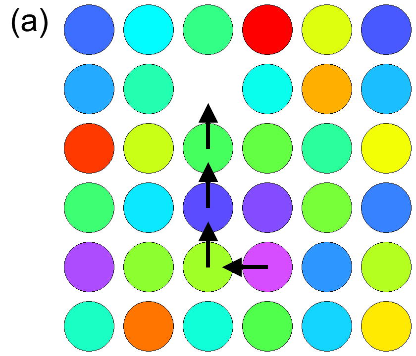
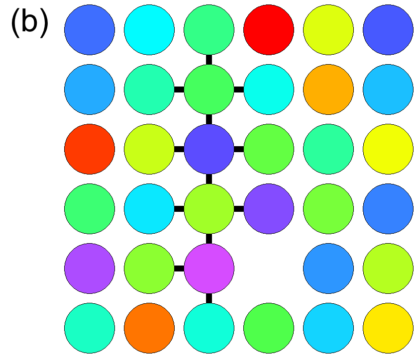
DPLM is defined by particles on a 2D square lattice of unit lattice constant and size with periodic boundary conditions. No more than one particle can occupy each site. Each particle is distinguishable from the others (see Fig. 1). For an occupied site , the particle index denotes which particle is at site . For convenience, we let if the site is unoccupied, i.e. occupied by a void. The occupation number is hence
| (1) |
where is the Kronecker delta. The whole set of , rather than , uniquely specifies the state of our system.
The total system energy is defined as
| (2) |
where the sum is over all nearest neighboring (NN) sites. It can be equivalently written as
| (3) |
where the sum is restricted to bonded NN sites and , i.e. with both sites occupied by particles.
A key feature is the site-particle-dependent interaction energy . Its dependence on particle indices and means that each particle defines its own interaction strengths and this will be justified further. Effectively, each particle is a type of its own generalizing multi-species models. In DPLM, each is time-independent and is an independent variable following a probability distribution except when the symmetry applies. We expect to be bounded below as in typical two particle interactions and thus should not be for example a simple Gaussian. For simplicity, is assumed to be the uniform distribution in which leads to a particle interaction slightly attractive on average.
To better understand the time-dependence of the interactions, it is instructive to write Eq. (3) as
| (4) |
where . We emphasize that while each interaction for any given sites and and particles and is a quenched random variable, the interaction at site and and arbitrary particles is quenched. Instead, admits an implicit time dependence via and , which are time dependent and change in values when a particle at or is replaced. Equally importantly, has no explicit time dependence. A previous value can thus be exactly reinstated whenever a previous local particle configuration as specified by and is restored via the return of the particles. We believe that such particle-dependent local interactions with persistent memory capture essential characteristics of structural glass. A further subtle point is that since depends on time, the disorder in our model is quenched in the physical space, unlike spin-glass models [6]. Instead, because of the time independence of and that the same interaction energy always applies to the same local particle configuration, the disorder is quenched in the configuration space.
This site-particle dependence in is not necessarily due to possible diverse particle properties. Instead, it effectively account for the impacts of positional disorder at sub-lattice resolutions which are usually truncated in lattice models. A particle at site in a spatially disordered system in principle admits a small random offset from the exact lattice point. This results in a random deviation in the atomic separation between the particles at sites and and hence also in the pair interaction . Rather than explicitly modeling the disorder in or , we directly consider the resulting random fluctuations in the interaction by simply taking a random . The dependence on both site and particle indices models the random changes expected to be induced by the hopping of any of the concerned particles or of the whole pair. Realistically, there must also be additional dependencies on further neighbors, which are all neglected for simplicity.
Equilibrium states of DPLM are exactly solvable. In particular, particle occupancies follow equilibrium statistics the same as those of a standard identical-particle lattice gas model with a constant interaction energy. These will be explained in Appendix A. Furthermore, equilibrium states of DPLM can be directly constructed using those of standard lattice gas, which exhibits no glassy slowdown (see Appendix B.5).
The dynamics of DPLM is defined by standard activated hopping approach for kinetic Monte Carlo simulations. Specifically, to simulate the dynamics at temperature , each particle can hop to an unoccupied NN site at a rate [25]
| (5) |
where is the change in the system energy due to the hop and is the Boltzmann constant. This definition satisfies detailed balance. We let so that . Also, we put without loss of generality. Particle motions can be equivalently described as void motions (see Fig. 1). At temperature , DPLM reduces to a simple sliding block model [26].
III Glassy dynamics
Let be the void density where is the particle density in principle related physically to the system pressure. We perform kinetic Monte Carlo simulations of fully equilibrated systems at at various and (see Appendix B for simulation methods). Standard dynamical measurements show that the system behaves as a simple liquid at high and and a glass at low and . As will be further explained, glassy behaviors are shown by the appearance of a plateau in the particle mean square displacement (MSD), a super-Arrhenius dependence of the particle diffusion coefficient , a stretched exponential form of the self-intermediate scattering function decaying towards zero at long time, a violation of the Stokes-Einstein relation, and typical time and dependences of a four-point susceptibility. In particular, the convergence of the self-intermediate scattering function towards zero rather than a finite value at long time verifies that DPLM is a model of structural glass, as opposed to for example spin glass. For all and studied, DPLM exhibits no sign of ideal glass transition. It also appears ergodic as supported, for example, by the divergence of the particle MSD and the vanishing of the self-intermediate scattering function at long time.
III.1 Diffusion coefficient
We calculate the MSD defined as where denotes the lattice position vector of particle at time . Figure 2(a) shows the MSD in a log-log plot for different and . For , the slopes of the lines are consistent with unity, indicating diffusive behavior over long observation time. Sub-diffusive plateaus appearing at intermediate at low indicate cage effects. Note that being a lattice model without vibrational modes at the sublattice level, the plateaus are much less pronounced as have been found for other lattice models [10].
From similar MSD for various and , we measure the particle diffusion coefficient
| (6) |
by fitting to data points where and the slope in the log-log plot is higher than 0.96. Fig. 2(b) shows in an Arrhenius plot for various . It exhibits super-Arrhenius behavior which becomes more pronounced at small and low . This shows that DPLM is a fragile glass.
III.2 Self-intermediate scattering function
We have measured the self-intermediate scattering function defined as
| (7) |
and the result is shown in Fig. 3(a) for and with . A one-step drop of versus instead of a two-step decay is again typical for lattice models [27, 10, 12]. In glassy systems, the terminal decay of the scattering function is usually well approximated by the Kohlrausch-Williams-Watts (KWW) stretched exponential function of the form , where is a relaxation time and () is the stretching exponent. Our results fit well to the KWW form for large . This is also demonstrated by the log-log plot of against in Fig. 3(b) which shows a linear region at large expected from the KWW form with . The stretching exponent obtained from the slope of the linear region is plotted in Fig. 4(a). As decreases, drops from 1 to around 0.82, indicating glassy dynamics at low .
From Fig. 3(a), we also extract a relaxation time which is the time at which . Fig. 4(b) plots against . The value clearly increases with decreasing and demonstrate a violation of the Stokes-Einstein relation expected for glasses.
III.3 Four-point correlation function
Close to the glass transition, one region in a glassy fluid can relax much faster than another one. This spatially inhomogeneous dynamical behavior is known as dynamic heterogeneity. To quantitatively study the heterogeneity in the persistence of the particle configuration, one can define an overlap function as
| (8) |
It measures how much particle moves during times and at a length scale . Note that the average overlap equals the self-intermediate scattering function . Each particle contributes to an overlap field defined by
| (9) |
Consider its spatial correlation
| (10) |
where the average is over the spatial origin and the starting time 0. measures the correlation of the fluctuations in the overlap function between two points that are separated by .
In the Fourier space, we get
| (11) | |||||
One can define the susceptibility as , which is simply the variance of the overlap function. can be interpreted as the typical size of correlated clusters in structural relaxation, thus an efficient measure of the degree of dynamic heterogeneity.
Fig. 5 shows from DPLM simulations. As is typical for structural glasses, for each temperature, has a peak, which shifts to larger times, and has a larger value when decreases. This reveals an increasing length scale of dynamic heterogeneity when the system cools down.
IV Emergent facilitation behaviors
Being an energetically non-trivial model with and independently and fully tunable, it exhibits much richer physics than purely kinetic models such as KCM. The particle diffusion coefficient shown in Fig 2(b) is replotted in Fig. 6(a) against . At each , the linear relation in the log-log plot at small suggests the power-law
| (13) |
Fig. 6(b) plots the scaling exponent as a function of . For the liquid state at high , we get indicating that each void moves independently [26]. This is supported by a video in the Supplemental Material [28] showing the motions of the voids as well as the particles at . It can be observed that voids diffuse independently. Figure 7(a) visualizes the same motions using void trajectories (thin lines). They appear slightly more compact than those of simple random walks due to the disorder. Particles with non-zero net displacements (pink and red) induced by the same void can be grouped into a cluster. Cluster sizes for different voids are relatively uniform. Voids are not trapped and travel throughout the whole system independently at longer times. Dynamic heterogeneity revealed via these clusters is weak.
We now explain that the low regime exhibits dynamic facilitation [19]. Fig. 6(b) shows that rises to 2 and beyond at low . The nonlinear scaling dictates that a void at small has arbitrarily small contributions to the dynamics. According to simple chemical kinetics, corresponds to motion dominated by pairs of coupled voids. This quantitatively shows an emergent dynamic facilitation behavior of void motions. It is analogous to KCM and in particular the spin facilitation dynamics of the FA model [8]. We have checked that the nonlinear scaling in Eq. (13) is not due to any void aggregation and is robust upon tuning the void-void attraction by a shift of the probability distribution on the energy scale.
To verify the above facilitation interpretation of Eq. (13), we directly visualize the particle motions for in a video in the Supplemental Material [28]. It can be seen that isolated voids are trapped. In sharp contrast, a pair of voids nearby to each other moves vigorously. Figure 7(b) shows the void trajectories in the same simulation which become very compact with numerous dead-ends indicating confined motions of the voids due to enhanced disorder. The trajectory of each isolated void induces no or few displaced particles (pink and red) as most particles have not hopped or have returned to their original positions. In contrast, the pair of voids nearby to each other induces significantly more extensive intertwining trajectories and vigorous particle displacements. Such pairs dominate the dynamics for the regime. At longer times, isolated voids typically remain trapped locally by the disorder unless visited and untrapped by other mobile pairs. Pairs of voids may split and new pairs may emerge but these occur at a longer time scale. Dynamic heterogeneity induced by highly mobile pairs of voids among trapped isolated voids is thus strong. Fig. 6(b) suggests that may reach 3 and beyond at even lower indicating dynamics dominated by triplets of voids, etc.


The dynamics of an isolated void at low typically involve motions confined along low-energy paths. Note that hops by a single void typically corresponds to single-hops by particles as shown in Fig. 1. A trapped void hence typically leads to bistable-like back-and-forth hops by a few particles. Such repetitive motions observed in MD simulations of polymers have been argued as the main cause of super-Arrhenius slow-down [29]. We have adapted the method in Ref. 29 to quantify these repetitions. Specifically, after a particle has hopped, we measure the probability that its next hop returns itself to the original site. The probability that it next hops instead to a new site is also measured. The results for are plotted in Fig. 8. They follow within 0.01% and the minor deviations are due to particles without a second hop during the observed period. At large , we find empirically that applicable for small noting that the random walks of voids induce correlated walks of particles [30]. We have checked that approaches towards the particle random walk value 1/4 at large . As decreases, increases monotonically reaching 0.96 for the lowest studied. The trend strikingly resembles those from polymer simulations [29]. This resemblance also strongly supports the physical relevance of DPLM. Such a high means that most hops are reversed and irrelevant to long-time dynamics. The repetition thus must contribute significantly to the slowdown. As , our results support . Most hopping particles then form two-level systems (TLS) known to be relevant to glass at very low [31].
V Conclusion
We have developed DPLM as a lattice gas model based on distinguishable particles for studying glassy dynamics. In the glassy phase, the particle diffusion coefficient scales nonlinearly with the void density in the low void density limit. This implies that isolated voids are essentially trapped and the dynamics of a void is dominated by facilitation by other voids nearby. Particle hopping becomes increasingly repetitive at low temperature.
DPLM is defined by a simple, generic, and physically motivated system energy function. It has both non-trivial energetics and kinetics. It can be efficiently simulated and equilibrium states can be directly generated at arbitrary temperature and density. Its glassy state does not rely on frustration on a specific lattice type. These may render DPLM a unique prototypical model for the further study of glassy dynamics and aging in disordered systems.
The definition of DPLM involves no explicit facilitation rule but facilitation behaviors are observed. It thus provides a strong microscopic support to dynamic facilitation and KCM. It will be interesting to deduce the precise coarse-grained lattice model for DPLM. Dynamic facilitation of voids demonstrated by DPLM is analogous to the picture of facilitation via pair-interactions of string-like particle motions motivated by MD simulations of polymers [29]. In that picture, each string is initiated by a single void leading to a one-one correspondence between strings and voids. From Fig. 1, the motion of a void alters the particle pairings and hence the energy landscape along its entire path. The energy landscape experienced by another void nearby is thus altered. Whether the second void can diffuse across the path of the first void is thus randomly affected. This demonstrates a form of path interaction of voids which is essentially equivalent to string interactions observed in MD [29]. The particle and void dynamics in DPLM as well as in polymer simulations is recently described on the same footing by a random local configuration tree theory [32]. Alternatively, it will also be of interest to study DPLM defined on the Bethe lattice which may allow exact analysis.
In DPLM, each is an independent random variable. More generally, Eq. (2) features a very generic Hamiltonian. Adopting instead a constant gives a simple interacting lattice gas. As lattice gas models can be mapped to spin models with spin-exchange (Kawasaki) dynamics, it also represents a ferromagnetic or anti-ferromagnetic spin model. Alternatively, a particle-dependent reduces it to a multi-species lattice gas such as a binary alloy [33]. Limiting to a site-dependent , it becomes a variant of the Edwards-Anderson (EA) model for spin glass [6] with Kawasaki dynamics and a random field. In addition, by continuously varying the correlations between the various , Eq. (2) describes models interpolating between these systems.
Acknowledgements.
We thank helpful discussions with J.Q. You, Ho-Kei Chan and Peter Harrowell. We are grateful to the support of Hong Kong GRF (Grant 15301014).Appendix A Exact equilibrium statistics
Assuming ergodicity, which is supported by our simulations in Sec. III, it is possible to derive exact equilibrium states of DPLM in the thermodynamic limit. This is because the system follows a Boltzmann distribution which factorizes over the bonds. More specifically, equilibrium statistics in the ergodic phase of a system with particles is described by the canonical partition function
| (14) |
where the sum is over all possible system states and . Noting that denotes a void, can be rewritten as
| (15) |
Here, the first sum is over all possible site occupancies with defined in Eq. (1). The second sum is over the set of the permutations of particle arrangement at the occupied sites with . Equation (15) can be recast into
| (16) |
where is the partition function restricted to the specific site occupation and is given by
| (17) |
after applying Eq. (3).
A.1 Quenched and annealed averaging
The value of primary interest is the quenched average where the bar denotes averaging over the time-independent variables . At sufficiently high , it may agree with the annealed average , where again denotes averaging over which is now reinterpreted as additional time-dependent system state variables. A detailed derivation of this agreement will be explained in Appendix A.2.
We first study annealed averages which are much easier to calculate. Applying annealed averaging to Eq. (17), we get
| (18) |
where we have noted that each has a distinct set of indices and are thus independent random numbers. Defining
| (19) |
can then be interpreted as the average free energy of a bond between two NN particles and is given by
| (20) |
Substituting Eq. (19) into Eq. (18), all terms in the sum become identical and this trivially gives
| (21) |
It further reduces to
| (22) |
where is the number of pairs of bonded particles for the given site occupation . Substituting into the annealed average of Eq. (16), we get
| (23) |
The factor results from the particle distinguishability and is related to the Gibb’s paradox [34]. It is irrelevant and can be omitted for canonical ensembles with a constant considered here. We thus redefine by multiplying with a factor and obtain
| (24) |
A.2 Averaging over permutations
As discussed above, it is valid to redefine with an additional factor . Specifically, we continue to adopt Eq. (16) while Eq. (17) is replaced by
| (25) |
The r.h.s. now involves explicitly an average over particle permutations among the occupied sites. We will now explain that this averages out all . This is because as emphasized in Eq. (4), with nontrivial indices and is not quenched. It indeed samples over many different as particles permute, in sharp contrast to the quenched at fixed indices.
Without loss of generality, assume that sites 1 and 2 are occupied nearest neighboring sites. We single out the permutations concerning sites 1 and 2, giving
where is the partition function for the remain sites excluding particles and defined as
| (27) |
Since all particles are statistically equivalent, the dependence of on and is a manifestation of random fluctuations resulting from the random . Assuming negligible fluctuations in at large , which will be justified later, we write and Eq. (A.2) reduces to
| (28) |
where is defined in Eq. (20). Repeating similar procedures, a factor is contributed by every bond and we get
| (29) |
analogous to Eq. (22) after irrelevant prefactors in the latter are dropped.
At finite , for a given set of deviates from the value in Eq. (29) with a magnitude characterized by the standard deviation . We will show that becomes negligible compared with as increases. At high , this is obvious because fluctuations of each factor in Eq. (25) is small. We thus focus only on the case of low . The deduction is non-trivial because terms in Eq. (25) are correlated and have large variances increasing with .
At low , a term in Eq. (25) is significant predominantly when all its factors are relatively large. We thus characterize each factor only by whether it is large or small via the approximation
| (30) |
where
| (31) |
with . Noting that the apriori probability density of is uniform in , we have constructed the approximation so that the average of is unchanged. In particular, the probability that is
| (32) |
Equation (25) is then approximated by
| (33) |
where
| (34) |
Here, equals the number of relevant particle permutations which contribute significantly to . For each of these permutations, it is easy to see that all interactions are within from the average value .
We now evaluate the statistical properties of by tackling the combinatorial problem of counting the relevant permutations. For simplicity, we illustrate further calculations for a fully occupied lattice with interactions only in the non-trivial dimension, but generalization is straightforward. First, there are ways to occupy site . For each choice, there are on average ways to occupy site in which . It is analogous for the other sites except for which contributes a factor because both and must be nonzero. The average of is thus
| (35) | |||||
As a consistency check, substituting Eq. (35) into Eq. (33) and assuming recovers Eq. (29).
More importantly, we now calculate the standard deviation of . For each of the ways to occupy site 1, the number of ways to occupy site follows a binomial distribution with a variance . Each of these choices at sites 1 and on average results at relevant ways to permute the remaining particles. Therefore, fluctuations at contribute a variance to given by
| (36) | |||||
where we have used Eq. (35). We next consider fluctuation at site 3 as a further example. For each of the on average ways to occupy sites 1 and 2, the number of ways to occupy site 3 follows a binomial distribution with a variance . Each of these choices at sites 1, 2 and 3 on average results at relevant ways to permute the remaining particles. Fluctuations at site thus contribute a variance to given by
| (37) | |||||
Fluctuations at other sites can be similarly calculated. Neglecting correlations between these fluctuations, we get which simplifies to
| (38) | |||||
For large , all but the first term are negligible and we get . Since according to Eq. (33), the standard deviation of is . In particular, we have
| (39) |
To verify this result, we have numerically performed direct enumeration of values of using either Eq. (25) or Eq. (33) for independent realizations of for and . In both cases, Eq. (39) is readily verified. As a further check of our method, we consider alternative interactions in the form , representing particle-dependent interactions as opposed to site-particle-dependent ones. Using analogous arguments, we find instead , which is also well verified numerically by direct enumeration.
It is straightforward to generalize Eq. (39) to arbitrary site occupancies in 2D. Therefore, for DPLM studied in this work, Eq. (29) admits corrections only of order and is essentially exact for large . Substituting Eq. (29) into Eq. (16), we get
| (40) |
where all -dependent correction terms are of higher orders in . Note that similar arguments also imply that defined in Eq. (27) has negligible fluctuations and this justifies the assumption used in deriving Eq. (28).
We emphasize that we have at this point performed the ensemble average over and in Eq. (40) have already become independent of due to the averaging over particle permutations. This is quite analogous to self-averaging behaviors exhibited by many systems. Here, sample to sample fluctuations of hence vanish and all quenched averaging becomes trivial, i.e. . A further comparison of Eq. (40) with Eq. (24) gives
| (41) |
This shows the identical statistical properties of quenched and annealed ensembles in the ergodic phase for large .
A.3 Equilibrium properties
Let be the partition function of a simple identical-particle lattice gas with a NN particle interaction energy . It is easy to see that is in fact identical to in Eq. (40), i.e.
| (42) |
Therefore, DPLM and simple lattice gas have exactly the same equilibrium particle occupation statistics despite the very different dynamics. A simple lattice gas has a gas-liquid phase transition at the vaporization temperature , which depends on and thus on the distribution . The lattice gas can be further mapped to the 2D Ising model with an exchange [33]. Applying Onsager’s solution for the 2D Ising model [34], we get
| (43) |
where is given in Eq. (20) evaluated at . Solving Eqs. (20) and (43) numerically, we get . We have verified this value of using small-scale DPLM simulations at e.g. . Since is below studied in our main simulations, the systems considered here correspond to lattice gases in the gaseous phase, in which particles are only slightly attractive and neither particles nor voids in dilute concentration aggregate.
We now derive the equilibrium distribution of the interactions for annealed ensembles, which is identical to that of quenched ensembles according to Eq. (41). Restricting our consideration to a given site occupancy . We study the equilibrium properties of the remaining state variables and . They follow the Boltzmann probability distribution
| (44) |
where the product is over all NN sites and and all particles and . Applying Eq. (3), we get
| (45) |
Here, the first product is restricted to bonded NN sites and . Thus, the realized interaction which describes an existing bond in the state follows the Boltzmann distribution
| (46) |
where is a normalization constant. The second product in Eq. (45) is over the complementary set of unrealized interactions which do not represent any existing bond in the state . This equation also implies that these unrealized interactions simply follow .
We now further derive some other useful results. Adopting annealed ensemble, all in the r.h.s. of Eq. (45) are dummy indices of identical independent variables. All permutations of are indeed equivalent and only amount to different labeling of the particles. To see this mathematically, we note that after integrating over all , we get a uniform probability distribution
| (47) |
demonstrating the equivalence of all permutations for annealed ensembles as expected.
Appendix B Simulation details
We will describe both elementary and accelerated simulation approaches, which have been checked to generate statistically identical results. Our main simulations are all performed using accelerated algorithms. Each of them at lattice size takes up to about 20 hours to run on an Intel Xeon processor core. Data for each set of values of and are typically averaged over 5 similar independent runs. Additional shorter runs recording particle positions at a higher time-resolution are also needed to obtain correlation data at short time.
B.1 Elementary kinetic Monte Carlo method
Simulations can be performed using standard kinetic Monte Carlo approach. At each time step , the following procedures can be performed:
- •
Randomly choose a site .
- •
Randomly choose a site which is a NN of .
- •
If and is false, reject this step.
- •
Accept particle hop from to with probability where is calculated using Eq. (5)
Here, must be small and satisfies for all possible configurations.
B.2 Rejection-free method
The simple kinetic Monte Carlo algorithm above is inefficient due to too many rejected move attempts. A rejection-free method [35] is much more efficient. Let be the number of voids. We optimize our algorithm for which is most demanding due to the slow dynamics. The number of possible hops is in general. The associated hopping rates are calculated using Eq. (5) and stored at the lowest level of a complete binary tree. Each parent node then stores the sum of the two immediate children. Note that an exchange of two voids is unphysical and is assigned a rate 0.
For each time step , one of the possible hops is randomly selected with a relative probability . It is straightforward to select the hop efficiently by randomly descending the binary tree using the node values as the relative probabilistic weights. The hop is then executed. A few hopping rates associated with the hopping particle and its neighbors are recalculated since the local configuration has changed. The binary tree is then also updated accordingly. It is easy to see that is time dependent and follows , where is the value at the root of the binary tree and equals the sum of all the rates [36].
B.3 Two-step interaction energy tabulation
A nontrivial point in the programming for DPLM is that the total number of is of order . This requires too much memory storage for large . For medium values of , can be sampled only when needed and stored using a hash data structure. In our main simulations with a large , it is necessary to adopt a two-step tabulation method to be explained below.
As an approximate scheme, we put
| (50) |
Here, each for site is an independent random permutation function mapping the set to itself. The function thus involves only order tabulated random numbers sampled from which are independent from each other except when the symmetry applies. Before simulation starts, the functions and are randomly sampled and stored. The memory requirement significantly decreases from order to order . The method do introduce some unwanted correlations between the ideally independent . However, we have checked in medium scale simulations that it gives results statistically identical to those using the hash-table method.
B.4 Elementary initial thermalization
A straightforward approach is to generate each independently from the probability distribution taking into account the symmetry . The system state is initialized at infinite temperature by putting each particle randomly onto an unoccupied site in the lattice with uniform probability. This gives and at time . Thermalization kinetic Monte Carlo steps, typically performed using the rejection-free method explained above, are then conducted at the target temperature until equilibrium is attained.
During thermalization, equilibrium is indicated by the stabilization of various statistical measures such as the average particle energy . We have checked numerically that equilibration can be performed successfully under various conditions and a particularly demanding example in the glassy phase is illustrated in Fig. 9(a). The solid curves show against from two typical runs for and . They stabilize towards the average equilibrium value given in Eq. (49). Figure 9(b) shows the evolution of the probability distribution of the realized interaction at time from the same runs. It crossovers smoothly from the initial distribution toward the equilibrium distribution in Eq. (46). From both Figs. 9(a) and (b), the system can be deemed equilibrium for the given and for . The results verify numerically Eq. (49) and Eq. (46). More importantly, they hence also verify the agreement between quenched and annealed averages used in their derivations.
B.5 Direct initialization method
System equilibration at large using thermalization Monte Carlo steps explained above can take very long runtime at low . This is a major difficulty for many lattice models and most MD simulations of glass. Being able to directly construct equilibrium states is thus a highly desirable property. This is possible for KCM with trivial energetics, non-spatial models [37, 38] and some frustrated spin models defined on triangular or related lattices [39]. It is also possible for MD simulations of a system with long-range shifted interactions [23, 24]. DPLM is in our knowledge the only finite-dimensional and energetically non-trivial lattice model of glass defined on a general lattice with this capability.
First, we calculate the particle occupancy and the particle index at every site . We start by simulating a simple identical-particle lattice gas because of the equivalent particle statistics (see Eq. (42)). It is performed with a constant NN particle interaction energy given in Eq. (20) and we use the same computer code for DPLM with reduced to the constant . Similar to the elementary initial thermalization approach described above, we initialize the particle positions randomly and then equilibrate the simple lattice gas by a thermalization run. It is computationally very efficient because of the absence of glassification at arbitrary . The thermalized particle positions give and at time . Note that due to the identical-particle nature of this part of the simulation, only is of interest. The precise particle permutation as specified by for the occupied sites is irrelevant because all permutations are equally probable (see Eq. (47)).
Second, we randomly generate from the annealed ensemble, which is statistically identical to the quenched ensemble (see Eq. (41)). Specifically, We sample all unrealized from the distribution while realized interactions appearing in the state are sampled from the Boltzmann distribution given by Eq. (46). This completes the generation of an equilibrium state at .
In Fig. 9(a), the two dashed curves show the particle energy from two typical runs using this direct initialization method. They support that the systems have attained equilibrium energy once constructed and this numerically verifies the method. Note that at finite , interactions from this approach differ in principle from that based on the elementary method in Appendix B.4 in which all interactions are sampled from . Nevertheless, since the total number of is of order while the number of bonds is of order , the fraction of realized interactions sampled from is only of order . The fraction thus approaches zero at large and this demonstrations the equivalence of the elementary and the direct methods. Even after using our two-step tabulation approximation in Eq. (50), the fraction increases to order and still vanishes for large . This approach of determining the particle arrangement and before generating the interaction is closely analogous to a planting method in Refs. 23, 24.
B.6 Software reliability
Correct software implementation is highly nontrivial because minor programming mistakes may affect the particle dynamics only occasionally and can be very difficult to spot. One helpful consistency check is to measure the probability distribution of the interaction energy at equilibrium and compare with the exact distribution in Eq. (46). We have also conducted more general Boltzmann distribution tests [36] by performing long simulations using a small lattice with all but several particles frozen. Then, only a few thousand different configurations will be realized. We measure the total occurrence durations and the system energies of all these configurations and make sure that the results agree with the Boltzmann distribution within the expected statistical errors. With these tests, we believe that our software implementation is highly reliable.
References
- [1] G. Biroli and J. P. Garrahan, J. Chem. Phys. 138, 12A301 (2013)
- [2] F. H. Stillinger and P. G. Debenedetti, Annu. Rev. Condens. Matter Phys. 4, 263 (2013)
- [3] L. Berthier and G. Biroli, Rev. Mod. Phys. 83, 587 (2011)
- [4] W. Kob and H. C. Andersen, Phys. Rev. E 51, 4626 (1995)
- [5] K. Kremer and G. S. Grest, J. Chem. Phys. 92, 5057 (1990)
- [6] S. F. Edwards and P. W. Anderson, Journal of Physics F: Metal Physics 5, 965 (1975)
- [7] T. R. Kirkpatrick and D. Thirumalai, Phys. Rev. B 36, 5388 (1987)
- [8] G. H. Fredrickson and H. C. Andersen, Phys. Rev. Lett. 53, 1244 (1984)
- [9] R. G. Palmer, D. L. Stein, E. Abrahams, and P. W. Anderson, Phys. Rev. Lett. 53, 958 (1984)
- [10] W. Kob and H. C. Andersen, Phys. Rev. E 48, 4364 (1993)
- [11] G. Biroli and M. Mézard, Phys. Rev. Lett. 88, 025501 (2001)
- [12] R. K. Darst, D. R. Reichman, and G. Biroli, J. Chem. Phys. 132, 044510 (2010)
- [13] N. B. Tito, J. E. Lipson, and S. T. Milner, Soft Matter 9, 3173 (2013)
- [14] T. R. Kirkpatrick, D. Thirumalai, and P. G. Wolynes, Phys. Rev. A 40, 1045 (1989)
- [15] T. R. Kirkpatrick and D. Thirumalai, Rev. Mod. Phys. 87, 183 (2015)
- [16] T. Kirkpatrick and D. Thirumalai, J. Phys. A 22, L149 (1989)
- [17] F. Ritort and P. Sollich, Adv. Phys. 52, 219 (2003)
- [18] J. P. Garrahan, P. Sollich, and C. Toninelli, Dynamical heterogeneities in glasses, colloids and granular media, edited by L. Berthier, G. Biroli, J.-P. Bouchaud, L. Cipelletti, and W. van Saarloosand (Oxford University Press)(2011)
- [19] D. Chandler and J. P. Garrahan, Annu. Rev. Phys. Chem. 61, 191 (2010)
- [20] S.-i. Sasa, Phys. Rev. Lett. 109, 165702 (2012)
- [21] G. L. Hunter and E. R. Weeks, Rep. Prog. Phys. 75, 066501 (2012)
- [22] R. Mari, F. Krzakala, and J. Kurchan, Phys. Rev. Lett. 103, 025701 (2009)
- [23] R. Mari and J. Kurchan, J. Chem. Phys. 135, 124504 (2011)
- [24] P. Charbonneau, Y. Jin, G. Parisi, and F. Zamponi, Proc. Natl. Acad. Sci. 111, 15025 (2014)
- [25] K. A. Fichthorn and M. Scheffler, Phys. Rev. Lett. 84, 5371 (2000)
- [26] Ajay and R. G. Palmer, J. Phys. A 23, 2139 (1990)
- [27] P. Harrowell, Phys. Rev. E 48, 4359 (1993)
- [28] See supplemental material at http://apricot.ap.polyu.edu.hk/dplm for videos showing particle dynamics in small-scale simulations at and .
- [29] C.-H. Lam, arXiv:1508.03153 (2015)
- [30] M. Brummelhuis and H. Hilhorst, J. Stat. Phys. 53, 249 (1988)
- [31] W. Phillips, Rep. Prog. Phys. 50, 1657 (1987)
- [32] C.-H. Lam, arXiv:1611.03586 (2016)
- [33] K. Binder, Zeitschrift für Physik 267, 313 (1974)
- [34] M. Toda, R. Kubo, and N. Saito, Statistical physics I: equilibrium statistical mechanics (Springer, Heidelberg, 1991)
- [35] A. Bortz, M. Kalos, and J. Lebowitz, Journal of Computational Physics 17, 10 (1975)
- [36] C.-H. Lam, M. Lung, and L. M. Sander, Journal of Scientific Computing 37, 73 (2008)
- [37] B. Derrida, Phys. Rev. Lett. 45, 79 (1980)
- [38] F. Ritort, Phys. Rev. Lett. 75, 1190 (1995)
- [39] M. Newman and C. Moore, Phys. Rev. E 60, 5068 (1999)