跳到论文正文
W Papers独立论文阅读器 arXiv:1608.05959 论文正文 计算阅读时间 · 0%
引用这篇论文根据当前论文元数据生成,正式投稿前建议核对。


License: arXiv.org perpetual non-exclusive license
arXiv:1608.05959v1 [quant-ph] 21 Aug 2016

Quantum state transfer for multi-input linear quantum systems

Naoki Yamamoto    Hendra I. Nurdin    Matthew R. James ††thanks: N. Yamamoto is with the Department of Applied Physics and Physico-Informatics, Keio University, Hiyoshi 3-14-1, Kohoku, Yokohama, Japan (e-mail: yamamoto@appi.keio.ac.jp). H. I. Nurdin is with School of Electrical Engineering and Telecommunications, UNSW Australia, Sydney NSW 2052, Australia (e-mail: h.nurdin@unsw.edu.au). M. R. James is with Research School of Engineering, The Australian National University, Canberra, ACT 0200, Australia (e-mail: Matthew.James@anu.edu.au). This work is supported by the Australian Research Council, the UNSW Australia Faculty of Engineering, and JSPS Grant-in-Aid No. 15K06151.
Abstract

Effective state transfer is one of the most important problems in quantum information processing. Typically, a quantum information device is composed of many subsystems with multi-input ports. In this paper, we develop a general theory describing the condition for perfect state transfer from the multi-input ports to the internal system components, for general passive linear quantum systems. The key notion used is the zero of the transfer function matrix. Application to entanglement generation and distribution in a quantum network is also discussed.

I Introduction

A quantum state transducer, that for instance transfers an optical state to a solid state, is an indispensable component contained in various types of quantum information processors. For instance, such a state transfer procedure is involved in every quantum memory architecture [1, 2, 3, 4], which is typically used for building a quantum repeater in quantum communication networks [5]. Towards a systematic and effective design of state transfer protocol, in [6] two of the authors developed a general theory for single-input and single-output (SISO) passive linear quantum systems [7, 8]; the result obtained is that the input state encoded in an appropriately shaped wave function can be perfectly transferred to the system. A remarkable fact is that such a wave function can be completely characterized in terms of the zeros of the transfer function of the system, which thus revealed a close connection between systems and control theory and the important task in quantum information science.

Based on this background, in this paper, we aim to extend the result of [6] to the case of multi-input and multi-output (MIMO) general linear passive systems. In fact the memory systems studied in the above-referred papers [1, 2, 3] are all MIMO systems. Also a hybridized system conducting frequency conversion between e.g. an optical cavity and a microwave circuit is essentially an MIMO system [9, 10, 11]. On the other hand, it is well known in classical systems and control theory [12] that extending the notion of zeros from the SISO case to the MIMO case is quite nontrivial. This is because in the MIMO case we are dealing with a transfer function matrix, and the zeros of this matrix can have several definitions; for instance, a transmission zero is defined as a complex number at which the rank of the transfer function matrix drops, while a blocking zero is a complex number at which the transfer function matrix becomes a zero matrix. Therefore, the goal of this paper is to deduce the condition for perfect state transfer and how that condition can be characterized by the zeros of the transfer function matrix.

Notation: for a matrix A=(ai​j)A=(a_{ij}), the symbols A†A^{\dagger}, A⊤A^{\top}, and A♯A^{\sharp} represent its Hermitian conjugate, transpose, and complex conjugation in elements of AA, respectively; i.e., A†=(aj​i∗)A^{\dagger}=(a_{ji}^{*}), A⊤=(aj​i)A^{\top}=(a_{ji}), and A♯=(ai​j∗)A^{\sharp}=(a^{*}_{ij}). For a matrix of operators we use the same notation, in which case ai​j∗a_{ij}^{*} denotes the adjoint to ai​ja_{ij}.

II Preliminaries

II-A Model of the system and input

Let us consider the following MIMO passive linear quantum system [7, 8]:

d​𝒂d​t=A​𝒂−C†​S​𝒃,𝒃~=C​𝒂+S​𝒃.\frac{d\mbox{\boldmath$a$}}{dt}=A\mbox{\boldmath$a$}-C^{\dagger}S\mbox{\boldmath$b$},~~~\tilde{\mbox{\boldmath$b$}}=C\mbox{\boldmath$a$}+S\mbox{\boldmath$b$}. (1)

Here 𝒂=[a1,…,an]⊤\mbox{\boldmath$a$}=[a_{1},\ldots,a_{n}]^{\top} is the vector of system annihilation operators. This system has mm input channels represented by the vector of field annihilation operators 𝒃=[b1,…,bm]⊤\mbox{\boldmath$b$}=[b_{1},\ldots,b_{m}]^{\top}, and 𝒃~\tilde{\mbox{\boldmath$b$}} is the corresponding output. These are infinite dimensional operators satisfying e.g. ai​(t)​aj∗​(t)−aj∗​(t)​ai​(t)=δi​j​∀ta_{i}(t)a_{j}^{*}(t)-a_{j}^{*}(t)a_{i}(t)=\delta_{ij}~\forall t and bi​(t)​bj∗​(t′)−bj∗​(t′)​bi​(t)=δi​j​δ​(t−t′)​∀t,t′b_{i}(t)b_{j}^{*}(t^{\prime})-b_{j}^{*}(t^{\prime})b_{i}(t)=\delta_{ij}\delta(t-t^{\prime})~\forall t,t^{\prime}. In the dynamical equation, C∈ℂm×nC\in{\mathbb{C}}^{m\times n} represents the system-field coupling; also A=−i​Ω−C†​C/2A=-i\Omega-C^{\dagger}C/2, where the n×nn\times n Hermitian matrix Ω=Ω†\Omega=\Omega^{\dagger} is related to the system Hamiltonian. Finally SS is a m×mm\times m unitary matrix, representing the scattering process of 𝒃b.

In the state transfer problem considered in this paper, we assume that the input is given by a continuous-mode single-photon field state. This state is defined in terms of the following annihilation and creation process operators:

B⁡(ξ)=∫−∞∞ξ∗​(t)​b​(t)​𝑑t,B∗​(ξ)=∫−∞∞ξ⁡(t)​b∗​(t)​𝑑t.B(\xi)=\int_{-\infty}^{\infty}\xi^{*}(t)b(t)dt,~~B^{*}(\xi)=\int_{-\infty}^{\infty}\xi(t)b^{*}(t)dt. (2)

ξ⁡(t)\xi(t) is an associated function in ℂ{\mathbb{C}}, representing the shape of the optical pulse field. Also ξ⁡(t)\xi(t) satisfies the normalization condition ∫−∞∞|ξ⁡(t)|2​𝑑t=1\int_{-\infty}^{\infty}|\xi(t)|^{2}dt=1. Due to this, B⁡(ξ)B(\xi) and B∗​(ξ)B^{*}(\xi) satisfy the relation B⁡(ξ)​B∗​(ξ)−B∗​(ξ)​B​(ξ)=1B(\xi)B^{*}(\xi)-B^{*}(\xi)B(\xi)=1. The continuous-mode single photon field state is produced by acting B∗​(ξ)B^{*}(\xi) on the vacuum field |0⟩f|{0}\rangle_{f} as follows [13, 14]:

|1ξ⟩f=B∗​(ξ)​|0⟩f=∫−∞∞ξ⁡(t)​b∗​(t)​𝑑t​|0⟩f.|{1_{\xi}}\rangle_{f}=B^{*}(\xi)|{0}\rangle_{f}=\int_{-\infty}^{\infty}\xi(t)b^{*}(t)dt|{0}\rangle_{f}. (3)

This is the continuous-mode version of the single-mode single-photon state |1⟩=a∗​|0⟩|{1}\rangle=a^{*}|{0}\rangle where a∗a^{*} is the single-mode creation operator and |0⟩|{0}\rangle is the ground state. Note that f​⟨1ξ|1ξ⟩f=1\mbox{}_{f}\langle{1_{\xi}}|{1_{\xi}}\rangle_{f}=1 holds due to the normalization condition of ξ⁡(t)\xi(t). Also from the relation f​⟨1ξ|​b∗​(t)​b​(t)​|1ξ⟩f=|ξ⁡(t)|2\mbox{}_{f}\langle{1_{\xi}}|b^{*}(t)b(t)|{1_{\xi}}\rangle_{f}=|\xi(t)|^{2}, ξ⁡(t)\xi(t) has the meaning of the wave function such that |ξ⁡(t)|2|\xi(t)|^{2} represents the probability of photo detection per unit time.

II-B Zeros of a passive linear system

The transfer function matrix of the system (1) is given by

G⁡(s)=[I−C​(s​I−A)−1​C†]​S.G(s)=[I-C(sI-A)^{-1}C^{\dagger}]S.

Here we give two definitions of zeros of a general m×mm\times m transfer function matrix G⁡(s)G(s) [12].

Definition 1: If there exist z∈ℂz\in{\mathbb{C}} and 𝒖∈ℂm\mbox{\boldmath$u$}\in{\mathbb{C}}^{m} such that G⁡(z)​𝒖=0G(z)\mbox{\boldmath$u$}=0, then zz is called a transmission zero.

Definition 2: If there exists z∈ℂz\in{\mathbb{C}} such that G⁡(z)=0G(z)=0, then zz is called a blocking zero.

The following three facts are used in this paper.

Fact 1: Suppose that z∈ℂz\in{\mathbb{C}} is a (blocking or transmission) zero of G⁡(s)G(s), and it is not a pole of G⁡(s)G(s). Then zz is an eigenvalue of −A†-A^{\dagger}.

Proof: Let us first consider the case of a blocking zero. This means there exists z∈ℂz\in{\mathbb{C}} such that [I−C​(z​I−A)−1​C†]​S=0[I-C(zI-A)^{-1}C^{\dagger}]S=0. Now let us define V:=(z​I−A)−1​C†​SV:=(zI-A)^{-1}C^{\dagger}S; then we have (z​I−A)​V​S†=C†(zI-A)VS^{\dagger}=C^{\dagger} and C​V=SCV=S. These two equations lead to (z​I−A)​V=C†​C​V(zI-A)V=C^{\dagger}CV and therefore (A+C†​C)​V=z​V(A+C^{\dagger}C)V=zV. Thus −A†​V=z​V-A^{\dagger}V=zV; note that zz is degenerated in the eigenspace span⁡(V){\rm span}(V).

The case of transmission zero is almost the same. The definition is that there exist z∈ℂz\in{\mathbb{C}} and 𝒖∈ℂm\mbox{\boldmath$u$}\in{\mathbb{C}}^{m} such that G⁡(s)​𝒖=[I−C​(z​I−A)−1​C†]​S​𝒖=0G(s)\mbox{\boldmath$u$}=[I-C(zI-A)^{-1}C^{\dagger}]S\mbox{\boldmath$u$}=0. Again define V:=(z​I−A)−1​C†​SV:=(zI-A)^{-1}C^{\dagger}S, which leads to (z​I−A)​V​S†=C†(zI-A)VS^{\dagger}=C^{\dagger} and C​V​𝒖=S​𝒖CV\mbox{\boldmath$u$}=S\mbox{\boldmath$u$}; hence we have (z​I−A)​V​𝒖=C†​C​V​𝒖(zI-A)V\mbox{\boldmath$u$}=C^{\dagger}CV\mbox{\boldmath$u$} and −A†​V​𝒖=z​V​𝒖-A^{\dagger}V\mbox{\boldmath$u$}=zV\mbox{\boldmath$u$}. Note from this the transmission-zero vector 𝒖u and the eigenvector of −A†-A^{\dagger}, 𝒗v, are connected by 𝒗=V​𝒖\mbox{\boldmath$v$}=V\mbox{\boldmath$u$}. This further yields S†​C​𝒗=S†​C​V​𝒖=S†​S​𝒖=𝒖S^{\dagger}C\mbox{\boldmath$v$}=S^{\dagger}CV\mbox{\boldmath$u$}=S^{\dagger}S\mbox{\boldmath$u$}=\mbox{\boldmath$u$}, hence 𝒖=S†​C​𝒗\mbox{\boldmath$u$}=S^{\dagger}C\mbox{\boldmath$v$}. □\Box

Fact 2: If AA is Hurwitz, then all (blocking or transmission) zeros of G⁡(s)G(s) are unstable zeros.

Proof: Let λ\lambda be an eigenvalue of AA, i.e. det(λ​I−A)=0{\det}(\lambda I-A)=0. This yields det(λ∗​I−A†)=0{\det}(\lambda^{*}I-A^{\dagger})=0. Then from Fact 1, a zero of G⁡(s)G(s), z, is given by z=−λ∗z=-\lambda^{*}. Hence Re⁡(z)=−Re⁡(λ)>0{\rm Re}(z)=-{\rm Re}(\lambda)>0. □\Box

Fact 3: If AA is Hurwitz, G⁡(s)G(s) always has a transmission zero.

Proof: We begin with the eigen-equation −A†​𝒗=z​𝒗-A^{\dagger}\mbox{\boldmath$v$}=z\mbox{\boldmath$v$}. Then from −A†=A+C†​C-A^{\dagger}=A+C^{\dagger}C, we have (A+C†​C)​𝒗=z​𝒗(A+C^{\dagger}C)\mbox{\boldmath$v$}=z\mbox{\boldmath$v$}. Now from Fact 2, zz is not an eigenvalue of AA, hence (z−A)−1(z-A)^{-1} always exists; thus we have 𝒗=(z−A)−1​C†​C​𝒗\mbox{\boldmath$v$}=(z-A)^{-1}C^{\dagger}C\mbox{\boldmath$v$}. This yields C​𝒗=C​(z−A)−1​C†​C​𝒗C\mbox{\boldmath$v$}=C(z-A)^{-1}C^{\dagger}C\mbox{\boldmath$v$} and further [I−C​(z−A)−1​C†]​C​𝒗=0[I-C(z-A)^{-1}C^{\dagger}]C\mbox{\boldmath$v$}=0. Therefore we end up with G⁡(z)​S†​C​𝒗=0G(z)S^{\dagger}C\mbox{\boldmath$v$}=0, meaning that there always exists a transmission zero. Note again we find the transmission-zero vector 𝒖u and the eigenvector 𝒗v are connected by 𝒖=S†​C​𝒗\mbox{\boldmath$u$}=S^{\dagger}C\mbox{\boldmath$v$}. □\Box

III General MIMO state transfer

In what follows we assume that AA is Hurwitz. Then the solution of the dynamics is given by

𝒂♯(0)=U∗𝒂♯(t0)U=−∫t00e−A♯​tC⊤S♯𝒃♯(t)dt,\mbox{\boldmath$a$}^{\sharp}(0)=U^{*}\mbox{\boldmath$a$}^{\sharp}(t_{0})U=-\int_{t_{0}}^{0}e^{-A^{\sharp}t}C^{\top}S^{\sharp}\mbox{\boldmath$b$}^{\sharp}(t)dt, (4)

where UU is the unitary operator describing the joint time evolution of the system and the field from the initial time t0t_{0} to the final time 00. In particular the initial time is assumed to be t0→−∞t_{0}\rightarrow-\infty. Let us define the matrix of functions

Ξ⁡(t)=[ξ1,1​(t)⋯ξ1,m​(t)⋮⋮ξn,1​(t)⋯ξn,m​(t)]\displaystyle\hskip-30.00005pt\Xi(t)=\left[\begin{array}[]{ccc}\xi_{1,1}(t)&\cdots&\xi_{1,m}(t)\\ \vdots&&\vdots\\ \xi_{n,1}(t)&\cdots&\xi_{n,m}(t)\\ \end{array}\right]
:=−e−A♯​t​C⊤​S♯​Θ​(−t).\displaystyle\hskip-11.99998pt:=-e^{-A^{\sharp}t}C^{\top}S^{\sharp}\Theta(-t). (9)

Θ⁡(−t)\Theta(-t) is the Heaviside step function taking 11 for t≤0t\leq 0 and 00 for t>0t>0. This matrix satisfies ∫−∞∞Ξ⁡(t)​Ξ​(t)†​𝑑t=I\int_{-\infty}^{\infty}\Xi(t)\Xi(t)^{\dagger}dt=I. Then we find

U∗​𝒂♯​(t0)​U=[U∗​a1∗​(t0)​U⋮U∗​an∗​(t0)​U]=∫t00Ξ⁡(t)​𝒃♯​(t)​𝑑t\displaystyle\hskip-30.00005ptU^{*}\mbox{\boldmath$a$}^{\sharp}(t_{0})U=\left[\begin{array}[]{c}U^{*}a_{1}^{*}(t_{0})U\\ \vdots\\ U^{*}a_{n}^{*}(t_{0})U\\ \end{array}\right]=\int_{t_{0}}^{0}\Xi(t)\mbox{\boldmath$b$}^{\sharp}(t)dt
=[B1∗​(ξ1,1)+⋯+Bm∗​(ξ1,m)⋮B1∗​(ξn,1)+⋯+Bm∗​(ξn,m)],\displaystyle\hskip 20.00003pt=\left[\begin{array}[]{c}B_{1}^{*}(\xi_{1,1})+\cdots+B_{m}^{*}(\xi_{1,m})\\ \vdots\\ B_{1}^{*}(\xi_{n,1})+\cdots+B_{m}^{*}(\xi_{n,m})\\ \end{array}\right],

where Bk∗​(ξi,j)B_{k}^{*}(\xi_{i,j}) is the continuous-mode creation process operator on the kkth input channel, defined by Eq. (2). This means that a special class of input field state can be perfectly transferred to the system. For instance let us consider the following entangled single-photon field state:

|Ψ⁡(t0)⟩f=|1ξ1,1(1)⟩f+⋯+|1ξ1,m(m)⟩f\displaystyle\hskip-30.00005pt|{\Psi(t_{0})}\rangle_{f}=|{1_{\xi_{1,1}}^{(1)}}\rangle_{f}+\cdots+|{1_{\xi_{1,m}}^{(m)}}\rangle_{f}
=|1ξ1,1,0,…,0⟩f+⋯+|0,…,0,1ξ1,m⟩f\displaystyle\hskip 8.00003pt=|{1_{\xi_{1,1}},0,\ldots,0}\rangle_{f}+\cdots+|{0,\ldots,0,1_{\xi_{1,m}}}\rangle_{f}
=[B1∗(ξ1,1)+⋯+Bm∗(ξ1,m)]|0,…,0⟩f,\displaystyle\hskip 8.00003pt=\Big[B_{1}^{*}(\xi_{1,1})+\cdots+B_{m}^{*}(\xi_{1,m})\Big]|{0,\ldots,0}\rangle_{f},

where the definition (3) is used. Also we define |1(j)⟩=|0,…,1,…,0⟩|{1^{(j)}}\rangle=|{0,\ldots,1,\ldots,0}\rangle with 11 appearing only in the jjth component. Note f​⟨Ψ⁡(t0)|Ψ⁡(t0)⟩f=1\mbox{}_{f}\langle{\Psi(t_{0})}|{\Psi(t_{0})}\rangle_{f}=1 due to ∫−∞∞Ξ⁡(t)​Ξ​(t)†​𝑑t=I\int_{-\infty}^{\infty}\Xi(t)\Xi(t)^{\dagger}dt=I. In this case, from Eq. (III), the final state of the whole system is calculated as

|Ψ(0)⟩=U|0,…,0⟩s|Ψ(t0)⟩f\displaystyle\hskip-20.00003pt|{\Psi(0)}\rangle=U|{0,\ldots,0}\rangle_{s}|{\Psi(t_{0})}\rangle_{f}
=U[B1∗(ξ1,1)+⋯+Bm∗(ξ1,m)]|0,…,0⟩s|0,…,0⟩f\displaystyle\hskip-11.99998pt=U\Big[B_{1}^{*}(\xi_{1,1})+\cdots+B_{m}^{*}(\xi_{1,m})\Big]|{0,\ldots,0}\rangle_{s}|{0,\ldots,0}\rangle_{f}
=U[B1∗(ξ1,1)+⋯+Bm∗(ξ1,m)]U∗|0,…,0⟩s|0,…,0⟩f\displaystyle\hskip-11.99998pt=U\Big[B_{1}^{*}(\xi_{1,1})+\cdots+B_{m}^{*}(\xi_{1,m})\Big]U^{*}|{0,\ldots,0}\rangle_{s}|{0,\ldots,0}\rangle_{f}
=a1∗(t0)|0,…,0⟩s|0,…,0⟩f=|1,0,…,0⟩s|0,…,0⟩f\displaystyle\hskip-11.99998pt=a_{1}^{*}(t_{0})|{0,\ldots,0}\rangle_{s}|{0,\ldots,0}\rangle_{f}=|{1,0,\ldots,0}\rangle_{s}|{0,\ldots,0}\rangle_{f}
=|1(1)⟩s|0,…,0⟩f.\displaystyle\hskip-11.99998pt=|{1^{(1)}}\rangle_{s}|{0,\ldots,0}\rangle_{f}.

This equation shows that the first mode of the system acquires the single photon from the field; i.e. perfect state transfer is realized.

More generally, if the input field state is given by

|Ψ⁡(t0)⟩f=x1​(|1ξ1,1(1)⟩f+⋯+|1ξ1,m(m)⟩f)\displaystyle\hskip-30.00005pt|{\Psi(t_{0})}\rangle_{f}=x_{1}\Big(|{1_{\xi_{1,1}}^{(1)}}\rangle_{f}+\cdots+|{1_{\xi_{1,m}}^{(m)}}\rangle_{f}\Big)
+⋯+xn(|1ξn,1(1)⟩f+⋯+|1ξn,m(m)⟩f)\displaystyle\hskip 21.00009pt+\cdots+x_{n}\Big(|{1_{\xi_{n,1}}^{(1)}}\rangle_{f}+\cdots+|{1_{\xi_{n,m}}^{(m)}}\rangle_{f}\Big)
=|1ξ1′(1)⟩f+⋯+|1ξm′(m)⟩f,\displaystyle\hskip 8.00003pt=|{1_{\xi^{\prime}_{1}}^{(1)}}\rangle_{f}+\cdots+|{1_{\xi^{\prime}_{m}}^{(m)}}\rangle_{f}, (18)

where ξj′=x1​ξ1,j+⋯+xn​ξn,j\xi^{\prime}_{j}=x_{1}\xi_{1,j}+\cdots+x_{n}\xi_{n,j} and xj∈ℂx_{j}\in{\mathbb{C}} an arbitrary coefficient satisfying ∑j=1n|xj|2=1\sum_{j=1}^{n}|x_{j}|^{2}=1, in this case the final state is

|Ψ(0)⟩=(x1|1(1)⟩s+⋯+xn|1(n)⟩s)|0,…,0⟩f.|{\Psi(0)}\rangle=\Big(x_{1}|{1^{(1)}}\rangle_{s}+\cdots+x_{n}|{1^{(n)}}\rangle_{s}\Big)|{0,\ldots,0}\rangle_{f}. (19)

Note that the pulse functions ξi,j​(t)\xi_{i,j}(t) do not depend on the (unknown) coefficients {xj}\{x_{j}\}; hence, if the single photon field state with classical information {xj}\{x_{j}\} can be prepared, which is a challenging task experimentally, then it can be perfectly transferred to the system.

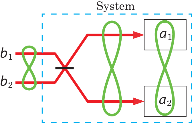
Example 1: Let us consider the case where the system is composed of two single-mode SISO subsystems specified by the system parameters (A1,C1)(A_{1},C_{1}) and (A2,C2)(A_{2},C_{2}). (Thus A1,A2,C1,C2A_{1},A_{2},C_{1},C_{2} are scalars.) These two subsystems can be placed at a distant location from a source. The two input fields are combined at a beam splitter before being sent to the two subsystems. Thus the whole system are specified by

A=[A100A2],C=[C100C2],S=[αββ−α].A=\left[\begin{array}[]{cc}A_{1}&0\\ 0&A_{2}\\ \end{array}\right],~~~C=\left[\begin{array}[]{cc}C_{1}&0\\ 0&C_{2}\\ \end{array}\right],~~~S=\left[\begin{array}[]{cc}\alpha&\beta\\ \beta&-\alpha\\ \end{array}\right].

Here α\alpha and β\beta represent the transmissivity and the reflectivity of the beam splitter, respectively, which are assumed to be real without loss of generality. Then we have

Ξ⁡(t)=[ξ1,1​(t)ξ1,2​(t)ξ2,1​(t)ξ2,2​(t)]\displaystyle\hskip-30.00005pt\Xi(t)=\left[\begin{array}[]{cc}\xi_{1,1}(t)&\xi_{1,2}(t)\\ \xi_{2,1}(t)&\xi_{2,2}(t)\\ \end{array}\right]
=[−α​e−A1∗​t​C1−β​e−A1∗​t​C1−β​e−A2∗​t​C2−α​e−A2∗​t​C2],\displaystyle\hskip-8.99994pt=\left[\begin{array}[]{cc}-\alpha e^{-A_{1}^{*}t}C_{1}&-\beta e^{-A_{1}^{*}t}C_{1}\\ -\beta e^{-A_{2}^{*}t}C_{2}&-\alpha e^{-A_{2}^{*}t}C_{2}\\ \end{array}\right],

and

[U∗​a1∗​(t0)​UU∗​a2∗​(t0)​U]=[B1∗​(ξ1,1)+B2∗​(ξ1,2)B1∗​(ξ2,1)+B2∗​(ξ2,2)].\left[\begin{array}[]{c}U^{*}a_{1}^{*}(t_{0})U\\ U^{*}a_{2}^{*}(t_{0})U\\ \end{array}\right]=\left[\begin{array}[]{c}B_{1}^{*}(\xi_{1,1})+B_{2}^{*}(\xi_{1,2})\\ B_{1}^{*}(\xi_{2,1})+B_{2}^{*}(\xi_{2,2})\\ \end{array}\right].

Then if the initial field state is prepared as

|Ψ(t0)⟩f=x1(|1ξ1,1,0⟩f+|0,1ξ1,2⟩f)\displaystyle\hskip-30.00005pt|{\Psi(t_{0})}\rangle_{f}=x_{1}\Big(|{1_{\xi_{1,1}},0}\rangle_{f}+|{0,1_{\xi_{1,2}}}\rangle_{f}\Big)
+x2(|1ξ2,1,0⟩f+|0,1ξ2,2⟩f)\displaystyle\hskip 40.00006pt\mbox{}+x_{2}\Big(|{1_{\xi_{2,1}},0}\rangle_{f}+|{0,1_{\xi_{2,2}}}\rangle_{f}\Big)
=|1x1​ξ1,1+x2​ξ2,1,0⟩f+|0,1x1​ξ1,2+x2​ξ2,2⟩f,\displaystyle\hskip 8.00003pt=|{1_{x_{1}\xi_{1,1}+x_{2}\xi_{2,1}},0}\rangle_{f}+|{0,1_{x_{1}\xi_{1,2}+x_{2}\xi_{2,2}}}\rangle_{f}, (26)

the final system state is given by

|Ψ(0)⟩s=x1|1,0⟩s+x2|0,1⟩s.|{\Psi(0)}\rangle_{s}=x_{1}|{1,0}\rangle_{s}+x_{2}|{0,1}\rangle_{s}.

That is, the two separately placed two subsystems are entangled. Note however that, to achieve the perfect state transfer, in general, the initial field state has to be entangled between the two input channels even before entering into the beam splitter. □\Box
Refer to caption
Fig. 1: Perfect state transfer from the field single-photon entangled state to the system single-photon entangled state.

IV Perfect state transfer and zeros

In the previous section we found that, in the general setup, the field state (18) can be perfectly transferred to the system state (19). That is, although engineering the entangled single-photon state (18) is challenging in experiment, perfect state transfer is in principle always possible. This can be understood in terms of systems and control theory as follows. In general, for a linear system if the input is of the form 𝒖⁡(t)=𝒖​ez​t\mbox{\boldmath$u$}(t)=\mbox{\boldmath$u$}e^{zt} with zz a transmission zero and 𝒖u the corresponding transmission-zero vector, then the output is given by 𝒚⁡(t)=G⁡(z)​𝒖​ez​t=0\mbox{\boldmath$y$}(t)=G(z)\mbox{\boldmath$u$}e^{zt}=0 for all t≤0t\leq 0. That is, if the system has a transmission (or more strongly blocking) zero, then an appropriately chosen input can make the output always zero. The point here is that the passive linear quantum system always has a transmission zero as shown in Fact 3, and this is the reason why the field state (18) is perfectly absorbed into the system. Thus the questions arising here are how the pulse function can be represented in terms of zeros of the system, and what field state represented in terms of zeros can be perfectly transferred.

To answer these questions let us recall Facts 1 and 3. That is, the system always has a transmission zero zz satisfying G⁡(z)​𝒖=0G(z)\mbox{\boldmath$u$}=0 with 𝒖u the corresponding transmission-zero vector, and this satisfies the eigen-equation −A†​𝒗=z​𝒗-A^{\dagger}\mbox{\boldmath$v$}=z\mbox{\boldmath$v$} with 𝒗v the corresponding eigenvector. Further, 𝒖u and 𝒗v are related as 𝒖=S†​C​𝒗\mbox{\boldmath$u$}=S^{\dagger}C\mbox{\boldmath$v$}. Therefore, from Eq. (4) we have

𝒗⊤𝒂♯(0)=−∫t00𝒗⊤e−A♯​tC⊤S♯𝒃♯(t)dt\displaystyle\hskip-30.00005pt\mbox{\boldmath$v$}^{\top}\mbox{\boldmath$a$}^{\sharp}(0)=-\int_{t_{0}}^{0}\mbox{\boldmath$v$}^{\top}e^{-A^{\sharp}t}C^{\top}S^{\sharp}\mbox{\boldmath$b$}^{\sharp}(t)dt
=−∫t00ez​t𝒗⊤C⊤S♯𝒃♯(t)dt\displaystyle\hskip 8.99994pt=-\int_{t_{0}}^{0}e^{zt}\mbox{\boldmath$v$}^{\top}C^{\top}S^{\sharp}\mbox{\boldmath$b$}^{\sharp}(t)dt
=−∫t00ez​t𝒖⊤𝒃♯(t)dt\displaystyle\hskip 8.99994pt=-\int_{t_{0}}^{0}e^{zt}\mbox{\boldmath$u$}^{\top}\mbox{\boldmath$b$}^{\sharp}(t)dt
=𝒖⊤​𝑩♯​(−ez​t)\displaystyle\hskip 8.99994pt=\mbox{\boldmath$u$}^{\top}\mbox{\boldmath$B$}^{\sharp}(-e^{zt})
=u1​B1∗​(−ez​t)+⋯+um​Bm∗​(−ez​t),\displaystyle\hskip 8.99994pt=u_{1}B_{1}^{*}(-e^{zt})+\cdots+u_{m}B_{m}^{*}(-e^{zt}), (27)

where we have defined

𝑩♯​(ξ)=[B1∗​(ξ),…,Bm∗​(ξ)]⊤.\mbox{\boldmath$B$}^{\sharp}(\xi)=[B_{1}^{*}(\xi),\ldots,B_{m}^{*}(\xi)]^{\top}.

Note that −ez​t-e^{zt} is not normalized, but let us keep this unnormalized pulse function to explicitly see the transmission zero zz. We here chose the following field input state:

|Ψ(t0)⟩f=𝒖⊤𝑩♯(−ez​t)|0,0,…,0⟩f\displaystyle\hskip-10.00002pt|{\Psi(t_{0})}\rangle_{f}=\mbox{\boldmath$u$}^{\top}\mbox{\boldmath$B$}^{\sharp}(-e^{zt})|{0,0,\ldots,0}\rangle_{f}
=[u1B1∗(−ez​t)+⋯+umBm∗(−ez​t)]|0,0,…,0⟩f\displaystyle\hskip 0.0pt=\Big[u_{1}B_{1}^{*}(-e^{zt})+\cdots+u_{m}B_{m}^{*}(-e^{zt})\Big]|{0,0,\ldots,0}\rangle_{f}
=u1​|1−ez​t(1)⟩f+⋯+um​|1−ez​t(m)⟩f.\displaystyle\hskip 0.0pt=u_{1}|{1_{-e^{zt}}^{(1)}}\rangle_{f}+\cdots+u_{m}|{1_{-e^{zt}}^{(m)}}\rangle_{f}.

Then the final system-field state is given by

|Ψ(0)⟩=U|0,…,0⟩s|Ψ(t0)⟩f\displaystyle\hskip-30.00005pt|{\Psi(0)}\rangle=U|{0,\ldots,0}\rangle_{s}|{\Psi(t_{0})}\rangle_{f}
=𝒖⊤U𝑩♯(−ez​t)U∗|0,…,0⟩s|0,…,0⟩f\displaystyle\hskip 0.0pt=\mbox{\boldmath$u$}^{\top}U\mbox{\boldmath$B$}^{\sharp}(-e^{zt})U^{*}|{0,\ldots,0}\rangle_{s}|{0,\ldots,0}\rangle_{f}
=𝒗⊤𝒂♯(t0)|0,…,0⟩s|0,…,0⟩f\displaystyle\hskip 0.0pt=\mbox{\boldmath$v$}^{\top}\mbox{\boldmath$a$}^{\sharp}(t_{0})|{0,\ldots,0}\rangle_{s}|{0,\ldots,0}\rangle_{f}
=[v1|1(1)⟩s+⋯+vn|1(n)⟩s]|0,…,0⟩f.\displaystyle\hskip 0.0pt=\Big[v_{1}|{1^{(1)}}\rangle_{s}+\cdots+v_{n}|{1^{(n)}}\rangle_{s}\Big]|{0,\ldots,0}\rangle_{f}.

Hence certainly the input pulse function needs to be of the rising exponential form specified by the transmission zero zz, in order to achieve the perfect state transfer. In particular, the input field state has coefficients specified by 𝒖u, and the final system state has coefficients specified by 𝒗v.

The generalization is straightforward. Let us consider the case where the system has m¯(≤m)\bar{m}~(\leq m) transmission zeros, z1,…,zm¯z_{1},\ldots,z_{\bar{m}}, with corresponding transmission-zero vectors 𝒖1,…,𝒖m¯\mbox{\boldmath$u$}_{1},\ldots,\mbox{\boldmath$u$}_{\bar{m}}. Then from Eq. (27) we have

[𝒗1⊤​𝒂♯​(0)⋮𝒗m¯⊤​𝒂♯​(0)]=[𝒖1⊤​𝑩♯​(−ez1​t)⋮𝒖m¯⊤​𝑩♯​(−ezm¯​t)]\displaystyle\hskip-25.00003pt\left[\begin{array}[]{c}\mbox{\boldmath$v$}_{1}^{\top}\mbox{\boldmath$a$}^{\sharp}(0)\\ \vdots\\ \mbox{\boldmath$v$}_{\bar{m}}^{\top}\mbox{\boldmath$a$}^{\sharp}(0)\\ \end{array}\right]=\left[\begin{array}[]{c}\mbox{\boldmath$u$}_{1}^{\top}\mbox{\boldmath$B$}^{\sharp}(-e^{z_{1}t})\\ \vdots\\ \mbox{\boldmath$u$}_{\bar{m}}^{\top}\mbox{\boldmath$B$}^{\sharp}(-e^{z_{\bar{m}}t})\\ \end{array}\right]
=[u1,1​B1∗​(−ez1​t)+⋯+u1,m​Bm∗​(−ez1​t)⋮um¯,1​B1∗​(−ezm¯​t)+⋯+um¯,m​Bm∗​(−ezm¯​t)],\displaystyle\hskip-15.00002pt=\left[\begin{array}[]{c}u_{1,1}B_{1}^{*}(-e^{z_{1}t})+\cdots+u_{1,m}B_{m}^{*}(-e^{z_{1}t})\\ \vdots\\ u_{{\bar{m}},1}B_{1}^{*}(-e^{z_{\bar{m}}t})+\cdots+u_{{\bar{m}},m}B_{m}^{*}(-e^{z_{\bar{m}}t})\\ \end{array}\right],

where 𝒖j=[uj,1,…,uj,m]⊤\mbox{\boldmath$u$}_{j}=[u_{j,1},\ldots,u_{j,m}]^{\top}. Now we set the field input state to be

|Ψ⁡(t0)⟩f\displaystyle\hskip-15.00002pt|{\Psi(t_{0})}\rangle_{f}
=[x1​𝒖1⊤​𝑩♯​(−ez1​t)+⋯+xm¯​𝒖m¯⊤​𝑩♯​(−ezm¯​t)]\displaystyle\hskip-8.00003pt=\Big[x_{1}\mbox{\boldmath$u$}_{1}^{\top}\mbox{\boldmath$B$}^{\sharp}(-e^{z_{1}t})+\cdots+x_{\bar{m}}\mbox{\boldmath$u$}_{\bar{m}}^{\top}\mbox{\boldmath$B$}^{\sharp}(-e^{z_{\bar{m}}t})\Big]
×|0,0,…,0⟩f\displaystyle\hskip 38.00008pt\times|{0,0,\ldots,0}\rangle_{f}
=[x1(u1,1B1∗(−ez1​t)+⋯+u1,mBm∗(−ez1​t))+⋯\displaystyle\hskip-8.00003pt=\Big[x_{1}\Big(u_{1,1}B_{1}^{*}(-e^{z_{1}t})+\cdots+u_{1,m}B_{m}^{*}(-e^{z_{1}t})\Big)+\cdots
+xm¯(um¯,1B1∗(−ezm¯​t)+⋯+um¯,mBm∗(−ezm¯​t))]\displaystyle\hskip 5.0pt\mbox{}+x_{\bar{m}}\Big(u_{{\bar{m}},1}B_{1}^{*}(-e^{z_{\bar{m}}t})+\cdots+u_{{\bar{m}},m}B_{m}^{*}(-e^{z_{\bar{m}}t})\Big)\Big]
×|0,0,…,0⟩f\displaystyle\hskip 38.00008pt\times|{0,0,\ldots,0}\rangle_{f}
=[B1∗(−x1u1,1ez1​t−⋯−xm¯um¯,1ezm¯​t)+⋯\displaystyle\hskip-8.00003pt=\Big[B_{1}^{*}(-x_{1}u_{1,1}e^{z_{1}t}-\cdots-x_{\bar{m}}u_{{\bar{m}},1}e^{z_{\bar{m}}t})+\cdots
+Bm∗(−x1u1,mez1​t−⋯−xm¯um¯,mezm¯​t)]\displaystyle\hskip 10.00002pt\mbox{}+B_{m}^{*}(-x_{1}u_{1,m}e^{z_{1}t}-\cdots-x_{\bar{m}}u_{{\bar{m}},m}e^{z_{\bar{m}}t})\Big]
×|0,0,…,0⟩f\displaystyle\hskip 38.00008pt\times|{0,0,\ldots,0}\rangle_{f}
=[B1∗(u1′)+⋯+Bm∗(um′)]|0,0,…,0⟩f\displaystyle\hskip-8.00003pt=\Big[B_{1}^{*}(u_{1}^{\prime})+\cdots+B_{m}^{*}(u_{m}^{\prime})\Big]|{0,0,\ldots,0}\rangle_{f}
=|1u1′(1)⟩f+⋯+|1um′(m)⟩f,\displaystyle\hskip-8.00003pt=|{1_{u_{1}^{\prime}}^{(1)}}\rangle_{f}+\cdots+|{1_{u_{m}^{\prime}}^{(m)}}\rangle_{f}, (39)

where x1,…,xm¯x_{1},\ldots,x_{\bar{m}} are arbitrary coefficients and

𝒖′​(t):=[u1′​(t)⋮um′​(t)]\displaystyle\hskip-33.99998pt\mbox{\boldmath$u$}^{\prime}(t):=\left[\begin{array}[]{c}u_{1}^{\prime}(t)\\ \vdots\\ u_{m}^{\prime}(t)\\ \end{array}\right]
=[−x1​u1,1​ez1​t−⋯−xm¯​um¯,1​ezm¯​t⋮−x1​u1,m​ez1​t−⋯−xm¯​um¯,m​ezm¯​t]\displaystyle\hskip-8.00003pt=\left[\begin{array}[]{c}-x_{1}u_{1,1}e^{z_{1}t}-\cdots-x_{\bar{m}}u_{{\bar{m}},1}e^{z_{\bar{m}}t}\\ \vdots\\ -x_{1}u_{1,m}e^{z_{1}t}-\cdots-x_{\bar{m}}u_{{\bar{m}},m}e^{z_{\bar{m}}t}\\ \end{array}\right]
=−x1​𝒖1​ez1​t−⋯−xm¯​𝒖m¯​ezm¯​t.\displaystyle\hskip-8.00003pt=-x_{1}\mbox{\boldmath$u$}_{1}e^{z_{1}t}-\cdots-x_{\bar{m}}\mbox{\boldmath$u$}_{\bar{m}}e^{z_{\bar{m}}t}. (48)

Then by defining the vector

𝒗′:=x1​𝒗1+⋯+xm¯​𝒗m¯,\mbox{\boldmath$v$}^{\prime}:=x_{1}\mbox{\boldmath$v$}_{1}+\cdots+x_{\bar{m}}\mbox{\boldmath$v$}_{\bar{m}}, (49)

we find that

𝒗′​⊤​𝒂♯​(0)=[x1​𝒗1⊤+⋯+xm¯​𝒗m¯⊤]​𝒂♯​(0)\displaystyle\hskip-33.99998pt\mbox{\boldmath$v$}^{\prime}\mbox{}^{\top}\mbox{\boldmath$a$}^{\sharp}(0)=[x_{1}\mbox{\boldmath$v$}_{1}^{\top}+\cdots+x_{\bar{m}}\mbox{\boldmath$v$}_{\bar{m}}^{\top}]\mbox{\boldmath$a$}^{\sharp}(0)
=x1​𝒖1⊤​𝑩♯​(−ez1​t)+⋯+xm¯​𝒖m¯⊤​𝑩♯​(−ezm¯​t)\displaystyle\hskip 8.00003pt=x_{1}\mbox{\boldmath$u$}_{1}^{\top}\mbox{\boldmath$B$}^{\sharp}(-e^{z_{1}t})+\cdots+x_{\bar{m}}\mbox{\boldmath$u$}_{\bar{m}}^{\top}\mbox{\boldmath$B$}^{\sharp}(-e^{z_{\bar{m}}t})

and thus the final system-field state is given by

|Ψ(0)⟩=U|0,…,0⟩s|Ψ(t0)⟩f\displaystyle\hskip-30.00005pt|{\Psi(0)}\rangle=U|{0,\ldots,0}\rangle_{s}|{\Psi(t_{0})}\rangle_{f}
=[x1𝒖1⊤U𝑩♯(−ez1​t)U∗+⋯\displaystyle\hskip 0.0pt=\Big[x_{1}\mbox{\boldmath$u$}_{1}^{\top}U\mbox{\boldmath$B$}^{\sharp}(-e^{z_{1}t})U^{*}+\cdots
+xm¯𝒖m¯⊤U𝑩♯(−ezm¯​t)U∗]|0,…,0⟩s|0,…,0⟩f\displaystyle\hskip 5.0pt\mbox{}+x_{\bar{m}}\mbox{\boldmath$u$}_{\bar{m}}^{\top}U\mbox{\boldmath$B$}^{\sharp}(-e^{z_{\bar{m}}t})U^{*}\Big]|{0,\ldots,0}\rangle_{s}|{0,\ldots,0}\rangle_{f}
=𝒗′⊤𝒂♯(t0)|0,…,0⟩s|0,…,0⟩f\displaystyle\hskip 0.0pt=\mbox{\boldmath$v$}^{\prime}\mbox{}^{\top}\mbox{\boldmath$a$}^{\sharp}(t_{0})|{0,\ldots,0}\rangle_{s}|{0,\ldots,0}\rangle_{f}
=[v1′|1(1)⟩s+⋯+vn′|1(n)⟩s]|0,…,0⟩f.\displaystyle\hskip 0.0pt=\Big[v^{\prime}_{1}|{1^{(1)}}\rangle_{s}+\cdots+v^{\prime}_{n}|{1^{(n)}}\rangle_{s}\Big]|{0,\ldots,0}\rangle_{f}. (50)

Summarizing, if the field input state is given by Eq. (39) with pulse functions (IV), then it is perfectly transferred to the system state given by Eq. (50) with coefficient (49); again, {𝒖j}\{\mbox{\boldmath$u$}_{j}\} are the transmission-zero vectors and {𝒗j}\{\mbox{\boldmath$v$}_{j}\} are the corresponding eigenvectors of −A†-A^{\dagger}. Note that, if we formally input Eq. (IV) to the associated classical system with transfer function matrix G⁡(s)G(s), then the corresponding formal output is given by

𝒚=−x1​G​(z1)​𝒖1​ez1​t−⋯−xm¯​G​(zm¯)​𝒖m¯​ezm¯​t=0.\mbox{\boldmath$y$}=-x_{1}G(z_{1})\mbox{\boldmath$u$}_{1}e^{z_{1}t}-\cdots-x_{\bar{m}}G(z_{\bar{m}})\mbox{\boldmath$u$}_{\bar{m}}e^{z_{\bar{m}}t}=0.

However, this does not mean that the input field state can be set for instance to the separable one |1u1′⟩f⊗⋯⊗|1um′⟩f|{1_{u_{1}^{\prime}}}\rangle_{f}\otimes\cdots\otimes|{1_{u_{m}^{\prime}}}\rangle_{f}; the input state we need to prepare is the entangled state (39).

Example 2 (continued from Example 1): The transfer function matrix is given by

G⁡(s)=[G1​(s)00G2​(s)]​[αββ−α]\displaystyle\hskip-31.0001ptG(s)=\left[\begin{array}[]{cc}G_{1}(s)&0\\ 0&G_{2}(s)\\ \end{array}\right]\left[\begin{array}[]{cc}\alpha&\beta\\ \beta&-\alpha\\ \end{array}\right]
=[α​G1​(s)β​G1​(s)β​G2​(s)−α​G2​(s)],\displaystyle\hskip-8.00003pt=\left[\begin{array}[]{cc}\alpha G_{1}(s)&\beta G_{1}(s)\\ \beta G_{2}(s)&-\alpha G_{2}(s)\\ \end{array}\right],

where

Gj​(s)=1−Cj​(s−Aj)−1​Cj†=1−|Cj|2s−Aj\displaystyle\hskip-31.0001ptG_{j}(s)=1-C_{j}(s-A_{j})^{-1}C_{j}^{\dagger}=1-\frac{|C_{j}|^{2}}{s-A_{j}}
=s−Aj−|Cj|2s−Aj.\displaystyle\hskip-3.00003pt=\frac{s-A_{j}-|C_{j}|^{2}}{s-A_{j}}.

Again note that (Aj,Cj)(A_{j},C_{j}) are scalars. Clearly Gj​(s)G_{j}(s) has a zero zj=Aj+|Cj|2z_{j}=A_{j}+|C_{j}|^{2}. Here we assume that the two subsystems are different and as a result they have two different zeros, i.e. z1≠z2z_{1}\neq z_{2}; but note G1​(z1)=0G_{1}(z_{1})=0 and G2​(z2)=0G_{2}(z_{2})=0. In this case, the transmission-zero vector corresponding to z1z_{1} is given by 𝒖1=[α,β]⊤\mbox{\boldmath$u$}_{1}=[\alpha,\beta]^{\top}, and also 𝒖2=[β,−α]⊤\mbox{\boldmath$u$}_{2}=[\beta,-\alpha]^{\top} for the case z2z_{2};

G⁡(z1)​𝒖1=[00β​G2​(z1)−α​G2​(z1)]​[αβ]=0,\displaystyle\hskip 0.0ptG(z_{1})\mbox{\boldmath$u$}_{1}=\left[\begin{array}[]{cc}0&0\\ \beta G_{2}(z_{1})&-\alpha G_{2}(z_{1})\\ \end{array}\right]\left[\begin{array}[]{c}\alpha\\ \beta\\ \end{array}\right]=0,
G⁡(z2)​𝒖2=[α​G1​(z2)β​G1​(z2)00]​[β−α]=0.\displaystyle\hskip 0.0ptG(z_{2})\mbox{\boldmath$u$}_{2}=\left[\begin{array}[]{cc}\alpha G_{1}(z_{2})&\beta G_{1}(z_{2})\\ 0&0\\ \end{array}\right]\left[\begin{array}[]{c}\beta\\ -\alpha\\ \end{array}\right]=0.

The corresponding eigenvector 𝒗1\mbox{\boldmath$v$}_{1} is given, from the proof of Fact 1, by

𝒗1=V1​𝒖1=(z1−A)−1​C†​S​𝒖1\displaystyle\hskip-13.39998pt\mbox{\boldmath$v$}_{1}=V_{1}\mbox{\boldmath$u$}_{1}=(z_{1}-A)^{-1}C^{\dagger}S\mbox{\boldmath$u$}_{1}
=[z1−A100z1−A2]−1​[C1∗00C2∗]\displaystyle\hskip 0.0pt=\left[\begin{array}[]{cc}z_{1}-A_{1}&0\\ 0&z_{1}-A_{2}\\ \end{array}\right]^{-1}\left[\begin{array}[]{cc}C_{1}^{*}&0\\ 0&C_{2}^{*}\\ \end{array}\right]
×[αββ−α]​[αβ]\displaystyle\hskip 20.00003pt\times\left[\begin{array}[]{cc}\alpha&\beta\\ \beta&-\alpha\\ \end{array}\right]\left[\begin{array}[]{c}\alpha\\ \beta\\ \end{array}\right]
=[1/C10],\displaystyle\hskip 0.0pt=\left[\begin{array}[]{c}1/C_{1}\\ 0\\ \end{array}\right],

and also 𝒗2=[0,1/C2]⊤\mbox{\boldmath$v$}_{2}=[0,1/C_{2}]^{\top}. Note that these are certainly eigenvectors of −A†-A^{\dagger}. Hence the input field state can be prepared to |Ψ(t0)⟩f=|1u1′,0⟩f+|0,1u2′⟩f|{\Psi(t_{0})}\rangle_{f}=|{1_{u_{1}^{\prime}},0}\rangle_{f}+|{0,1_{u_{2}^{\prime}}}\rangle_{f} with pulse function

𝒖′​(t)=[u1′​(t)u2′​(t)]=−x1​𝒖1​ez1​t−x2​𝒖2​ez2​t\displaystyle\hskip 0.0pt\mbox{\boldmath$u$}^{\prime}(t)=\left[\begin{array}[]{c}u_{1}^{\prime}(t)\\ u_{2}^{\prime}(t)\\ \end{array}\right]=-x_{1}\mbox{\boldmath$u$}_{1}e^{z_{1}t}-x_{2}\mbox{\boldmath$u$}_{2}e^{z_{2}t}
=−x1​[αβ]​ez1​t−x2​[β−α]​ez2​t,\displaystyle\hskip 23.99997pt=-x_{1}\left[\begin{array}[]{c}\alpha\\ \beta\\ \end{array}\right]e^{z_{1}t}-x_{2}\left[\begin{array}[]{c}\beta\\ -\alpha\\ \end{array}\right]e^{z_{2}t},

and the system final state is then given by |Ψ(0)⟩s=v1′|1,0⟩s+v2′|0,1⟩s|{\Psi(0)}\rangle_{s}=v^{\prime}_{1}|{1,0}\rangle_{s}+v^{\prime}_{2}|{0,1}\rangle_{s} with 𝒗′=x1​𝒗1+x2​𝒗2\mbox{\boldmath$v$}^{\prime}=x_{1}\mbox{\boldmath$v$}_{1}+x_{2}\mbox{\boldmath$v$}_{2}. □\Box

V Separable input field

As mentioned before, the input field state (e.g. Eq. (18)) is in general entangled among input channels and is not always easy to generate in experiment. Hence it is reasonable to seek some conditions for perfect state transfer such that the input field state can be prepared relatively easily; in particular here we focus on a separable state such as |1ez​t,0,…,0⟩f|{1_{e^{zt}},0,\ldots,0}\rangle_{f}.

The first condition is, as expected, that the system has a blocking zero zz. In this case, as seen in Eq. (27), 𝒂∗​(0)\mbox{\boldmath$a$}^{*}(0) can be represented in terms of zz as follows; that is, using the relation C​V=SCV=S found in the proof of Fact 1, Eq. (4) yields

V⊤𝒂♯(0)=−∫t00V⊤e−A♯​tC⊤S♯𝒃♯(t)dt\displaystyle\hskip-25.00003ptV^{\top}\mbox{\boldmath$a$}^{\sharp}(0)=-\int_{t_{0}}^{0}V^{\top}e^{-A^{\sharp}t}C^{\top}S^{\sharp}\mbox{\boldmath$b$}^{\sharp}(t)dt
=−∫t00ez​tV⊤C⊤S♯𝒃♯(t)dt=−∫t00ez​t𝒃♯(t)dt\displaystyle\hskip 16.00008pt=-\int_{t_{0}}^{0}e^{zt}V^{\top}C^{\top}S^{\sharp}\mbox{\boldmath$b$}^{\sharp}(t)dt=-\int_{t_{0}}^{0}e^{zt}\mbox{\boldmath$b$}^{\sharp}(t)dt
=𝑩♯​(−ez​t)=[B1∗​(−ez​t)⋮Bm∗​(−ez​t)].\displaystyle\hskip 16.00008pt=\mbox{\boldmath$B$}^{\sharp}(-e^{zt})=\left[\begin{array}[]{c}B_{1}^{*}(-e^{zt})\\ \vdots\\ B_{m}^{*}(-e^{zt})\\ \end{array}\right].

Hence by introducing the normalized pulse function ζ⁡(t)=−z+z∗​ez​t\zeta(t)=-\sqrt{z+z^{*}}e^{zt}, which satisfies ∫−∞0|ζ⁡(t)|2​𝑑t=1\int_{-\infty}^{0}|\zeta(t)|^{2}dt=1, we have

z+z∗​V⊤​𝒂♯​(0)=𝑩♯​(ζ).\sqrt{z+z^{*}}V^{\top}\mbox{\boldmath$a$}^{\sharp}(0)=\mbox{\boldmath$B$}^{\sharp}(\zeta).

A remarkable feature of this relation is that the field operators are “disentangled”, unlike Eqs. (III) and (IV) which has the form of entangled operators, X1⊗I⊗⋯⊗I+⋯+I⊗⋯⊗I⊗XmX_{1}\otimes I\otimes\cdots\otimes I+\cdots+I\otimes\cdots\otimes I\otimes X_{m}. This means that a separable input field state can be chosen. For instance, let us consider

|Ψ(t0)⟩f=B1∗(ζ)|0,0,…,0⟩f=|1ζ,0,…,0⟩f.|{\Psi(t_{0})}\rangle_{f}=B_{1}^{*}(\zeta)|{0,0,\ldots,0}\rangle_{f}=|{1_{\zeta},0,\ldots,0}\rangle_{f}.

Then the system final state is given by

|Ψ(0)⟩s=𝒗1⊤𝒂♯(t0)|0,0,…,0⟩s\displaystyle\hskip-23.99997pt|{\Psi(0)}\rangle_{s}=\mbox{\boldmath$v$}_{1}^{\top}\mbox{\boldmath$a$}^{\sharp}(t_{0})|{0,0,\ldots,0}\rangle_{s}
=v1,1|1,0,…,0⟩s+⋯+v1,n|0,0,…,1⟩s,\displaystyle\hskip 10.00002pt=v_{1,1}|{1,0,\ldots,0}\rangle_{s}+\cdots+v_{1,n}|{0,0,\ldots,1}\rangle_{s},

where 𝒗1=[v1,1,…,v1,n]⊤\mbox{\boldmath$v$}_{1}=[v_{1,1},\ldots,v_{1,n}]^{\top} is the first column vector of z+z∗​V\sqrt{z+z^{*}}V. That is, if the system has a blocking zero, then a separable field state can be used to achieve the perfect state transfer.
Refer to caption
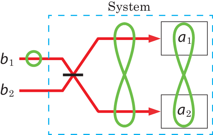
Fig. 2: Schematic for entanglement creation and distribution, which stems from a single photon field state with engineered pulse shape.

Example 3 (continued from Example 2): If the two subsystems are identical, i.e. A1=A2A_{1}=A_{2}, C1=C2C_{1}=C_{2}, then the two transfer functions become equal, G1​(s)=G2​(s)G_{1}(s)=G_{2}(s). Hence the whole transfer function matrix is given by

G⁡(s)=[α​G1​(s)β​G1​(s)β​G1​(s)−α​G1​(s)].G(s)=\left[\begin{array}[]{cc}\alpha G_{1}(s)&\beta G_{1}(s)\\ \beta G_{1}(s)&-\alpha G_{1}(s)\\ \end{array}\right].

Clearly in this case the system has a blocking zero, zz, satisfying G1​(z)=0G_{1}(z)=0, which is equal to z=A1+|C1|2z=A_{1}+|C_{1}|^{2}. Then the VV matrix appearing in Eq. (V) is given by

V=(z−A)−1​C†​S\displaystyle\hskip-13.99995ptV=(z-A)^{-1}C^{\dagger}S
=[z1−A100z1−A1]−1​[C1∗00C1∗]​[αββ−α]\displaystyle\hskip-3.00003pt=\left[\begin{array}[]{cc}z_{1}-A_{1}&0\\ 0&z_{1}-A_{1}\\ \end{array}\right]^{-1}\left[\begin{array}[]{cc}C_{1}^{*}&0\\ 0&C_{1}^{*}\\ \end{array}\right]\left[\begin{array}[]{cc}\alpha&\beta\\ \beta&-\alpha\\ \end{array}\right]
=1C1​[αββ−α].\displaystyle\hskip-3.00003pt=\frac{1}{C_{1}}\left[\begin{array}[]{cc}\alpha&\beta\\ \beta&-\alpha\\ \end{array}\right].

Therefore, if we prepare the field initial state as

|Ψ(t0)⟩f=B1∗(ζ)|0,0⟩f=|1ζ,0⟩f,|{\Psi(t_{0})}\rangle_{f}=B_{1}^{*}(\zeta)|{0,0}\rangle_{f}=|{1_{\zeta},0}\rangle_{f},

then the system final state is given by

|Ψ(0)⟩s=α|1,0⟩s+β|0,1⟩s,|{\Psi(0)}\rangle_{s}=\alpha|{1,0}\rangle_{s}+\beta|{0,1}\rangle_{s},

where we have used the fact that |z+z∗/C1|=1|\sqrt{z+z^{*}}/C_{1}|=1.

Note again that in this case we only need to prepare a single photon field state living in one channel; then this state becomes entangled after being combined at the beam splitter, and further it is perfectly transferred to the two identical systems, which can be spatially separated as shown in Fig. 2. That is, the schematic proposed here can be used for the purpose of creating and distributing entanglement in a quantum network. Specifically, it can be applied for constructing quantum repeaters [5] to realize a long-distance quantum communication. □\Box

Another condition such that a separable field input state can be perfectly transferred is as follows; if the transmission-zero vector 𝒖u appearing in Eq. (27) is e.g. of the form 𝒖=[1,0,…,0]⊤\mbox{\boldmath$u$}=[1,0,\ldots,0]^{\top}, then Eq. (27) gives

𝒗⊤​𝒂♯​(0)=B1∗​(−ez​t),\mbox{\boldmath$v$}^{\top}\mbox{\boldmath$a$}^{\sharp}(0)=B_{1}^{*}(-e^{zt}),

or equivalently −z+z∗​𝒗⊤​𝒂♯​(0)=B1∗​(ζ)-\sqrt{z+z^{*}}\mbox{\boldmath$v$}^{\top}\mbox{\boldmath$a$}^{\sharp}(0)=B_{1}^{*}(\zeta) with the normalized rising exponential function ζ⁡(t)=−z+z∗​ez​t\zeta(t)=-\sqrt{z+z^{*}}e^{zt}. In this case, the separable initial field state |Ψ(t0)⟩f=|1ζ,0,…,0⟩f|{\Psi(t_{0})}\rangle_{f}=|{1_{\zeta},0,\ldots,0}\rangle_{f} can be perfectly transferred to the system and the final system state is |Ψ⁡(0)⟩s=v1′​|1(1)⟩s+⋯+v1′​|1(n)⟩s|{\Psi(0)}\rangle_{s}=v^{\prime}_{1}|{1^{(1)}}\rangle_{s}+\cdots+v^{\prime}_{1}|{1^{(n)}}\rangle_{s} with vj′v_{j}^{\prime} the jjth component of the vector −z+z∗​𝒗-\sqrt{z+z^{*}}\mbox{\boldmath$v$}.

Refer to caption
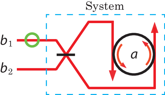
Fig. 3: Single photon absorption into the single-mode ring-resonator with two wave guides.

Example 4: Let us consider the system studied in [15], depicted in Fig. 3. The system is a single-mode ring resonator coupled to two optical waveguides, hence it is a 2-input and 2-output system. The wave guides are combined at a beam splitter before connected to the resonator. The transfer function of this system is given by

G⁡(s)=1s+(γ1+γ2)/2\displaystyle\hskip-13.99995ptG(s)=\frac{1}{s+(\gamma_{1}+\gamma_{2})/2}
×[s+(γ2−γ1)/2−γ1​γ2−γ1​γ2s+(γ1−γ2)/2]​[αββ−α],\displaystyle\hskip-3.00003pt\times\left[\begin{array}[]{cc}s+(\gamma_{2}-\gamma_{1})/2&-\sqrt{\gamma_{1}\gamma_{2}}\\ -\sqrt{\gamma_{1}\gamma_{2}}&s+(\gamma_{1}-\gamma_{2})/2\\ \end{array}\right]\left[\begin{array}[]{cc}\alpha&\beta\\ \beta&-\alpha\\ \end{array}\right],

where γ1\gamma_{1} and γ2\gamma_{2} are coupling constants between the resonator and the waveguides. Also α\alpha and β\beta are the transmissivity and the reflectivity of the beam splitter, respectively. Clearly G⁡(s)G(s) does not have a blocking zero, but (as guaranteed by Fact 3) it has a transmission zero z=(γ1+γ2)/2z=(\gamma_{1}+\gamma_{2})/2 with corresponding transmission-zero vector

𝒖=[αββ−α]​[γ1γ2]=[α​γ1+β​γ2β​γ1−α​γ2].\mbox{\boldmath$u$}=\left[\begin{array}[]{cc}\alpha&\beta\\ \beta&-\alpha\\ \end{array}\right]\left[\begin{array}[]{c}\sqrt{\gamma_{1}}\\ \sqrt{\gamma_{2}}\\ \end{array}\right]=\left[\begin{array}[]{c}\alpha\sqrt{\gamma_{1}}+\beta\sqrt{\gamma_{2}}\\ \beta\sqrt{\gamma_{1}}-\alpha\sqrt{\gamma_{2}}\\ \end{array}\right].

Therefore from the result of Section IV we need to prepare the following (unnormalized) entangled input field state:

|Ψ(t0)⟩f=(αγ1+βγ2)|1ez​t,0⟩f\displaystyle\hskip-13.99995pt|{\Psi(t_{0})}\rangle_{f}=(\alpha\sqrt{\gamma_{1}}+\beta\sqrt{\gamma_{2}})|{1_{e^{zt}},0}\rangle_{f}
+(βγ1−αγ2)|0,1ez​t⟩f,\displaystyle\hskip 30.00005pt\mbox{}+(\beta\sqrt{\gamma_{1}}-\alpha\sqrt{\gamma_{2}})|{0,1_{e^{zt}}}\rangle_{f},

to achieve the perfect state transfer. However, in the special case where the parameters satisfy the condition β​γ1−α​γ2=0\beta\sqrt{\gamma_{1}}-\alpha\sqrt{\gamma_{2}}=0, which leads to 𝒖=[1,0]⊤\mbox{\boldmath$u$}=[1,0]^{\top}, we only need to prepare a separable input field state |Ψ(t0)⟩f=|1ez​t,0⟩f|{\Psi(t_{0})}\rangle_{f}=|{1_{e^{zt}},0}\rangle_{f}, and it is perfectly transferred to the system (see Fig. 3). Note that in this case, because the system is single-mode, the final system state is merely |1⟩s|{1}\rangle_{s}. □\Box

VI Conclusion

In this paper, we first showed that the MIMO passive linear system always has a transmission zero, which ensures that a field single-photon state with appropriately engineered pulse function can be perfectly transferred to the system. Although in general the field state has to be an entangled state, under additional specific condition, this requirement can be relaxed; that is, as proven in Section V, a separable field state can be perfectly transferred to the system. This leads to a convenient schematic for creating and distributing entanglement in a quantum network.

References

  • [1] A. W. Elshaari, A. Aboketaf, and S. F. Preble, Controlled storage of light in silicon cavities, Opt. Express 18-3, 3014, 2010.
  • [2] D. E. Chang, A. H. Safavi-Naeini, M. Hafezi, and O. Painter, Slowing and stopping light using an optomechanical crystal array, New J. Phys. 13, 023003, 2011.
  • [3] K. Jensen et. al., Quantum memory for entangled continuous-variable states, Nature Physics 7, 13, 2011.
  • [4] Focus on quantum memory, Ed. by G. Brennen, E. Giacobino, and C. Simon, New J. Phys. 2013.
  • [5] N. Sangouard, C. Simon, H. de Riedmatten, and N. Gisin, Quantum repeaters based on atomic ensembles and linear optics, Rev. Mod. Phys. 83, 1, 2011.
  • [6] N. Yamamoto and M. R. James, Zero-dynamics principle for perfect quantum memory in linear networks, New J. Phys. 16, 073032, 2014.
  • [7] J. E. Gough, R. Gohm, and M. Yanagisawa, Linear quantum feedback networks, Phys. Rev. A 78, 062104, 2008.
  • [8] M. Guta and N. Yamamoto, Systems identification for passive linear quantum systems: the transfer function approach, IEEE Trans. Automat. Contr. 61-4, 921/936, 2016.
  • [9] A. H. Safavi-Naeini and O. Painter, Proposal for an optomechanical traveling wave phonon-photon translator, New J. Phys. 13, 013017, 2011.
  • [10] Y-D. Wang and A. A. Clerk, Using interference for high fidelity quantum state transfer in optomechanics, Phys. Rev. Lett. 108, 153603, 2012.
  • [11] R. Hisatomi et. al., Bidirectional conversion between microwave and light via ferromagnetic magnons, Phys. Rev. B 93, 174427, 2016.
  • [12] K. Zhou and J. C. Doyle, Essentials of Robust Control, Prentice Hall, 1997.
  • [13] K. M. Gheri, K. Ellinger, T. Pellizzari, and P. Zoller, Photon-wavepackets as flying quantum bits, Fortschr. Phys. 46, 4-5, 401/415, 1998.
  • [14] G. J. Milburn, Coherent control of single photon states, Eur. Phys. J. 159, 113/117, 2008.
  • [15] S. Huang and G. S. Agarwal, Coherent perfect absorption of path entangled single photons, Optics Express, 22-17, 20936, 2014.