Non-singular Brans-Dicke collapse in deformed phase space
Abstract
We study the collapse process of a homogeneous perfect fluid (in FLRW background) with a barotropic equation of state in Brans-Dicke (BD) theory in the presence of phase space deformation effects. Such a deformation is introduced as a particular type of non-commutativity between phase space coordinates. For the commutative case, it has been shown in the literature , that the dust collapse in BD theory leads to the formation of a spacetime singularity which is covered by an event horizon. In comparison to general relativity (GR), the authors concluded that the final state of black holes in BD theory is identical to the GR case but differs from GR during the dynamical evolution of the collapse process. However, the presence of non-commutative effects influences the dynamics of the collapse scenario and consequently a non-singular evolution is developed in the sense that a bounce emerges at a minimum radius, after which an expanding phase begins. Such a behavior is observed for positive values of the BD coupling parameter. For large positive values of the BD coupling parameter, when non-commutative effects are present, the dynamics of collapse process differs from the GR case. Finally, we show that for negative values of the BD coupling parameter, the singularity is replaced by an oscillatory bounce occurring at a finite time, with the frequency of oscillation and amplitude being damped at late times.
Keywords:
Brans-Dicke theory, Noncommutative geometry, Gravitational collapse, Spaceetime singularitypacs
04.50.Kd, 02.40.Gh, 04.70.Bw, 04.20.DwI Introduction
The general theory of relativity proposed by Albert Einstein provides a comprehensive and coherent description of gravity at the level of large-scale interactions. It is a geometrical theory which is formulated in such a way that space and time are not the absolute entities of classical mechanics, but rather, dynamical quantities determined together with the distribution and motion of matter and energy. Notwithstanding the successes and experimental validations, in the last thirty years several shortcomings of GR were nevertheless found leaving the scientists with the idea that there is no reason to believe that GR is the only fundamental theory of gravitation [1]. Among the alternative theories to GR, the BD theory [2] is one of the simplest and well studied generalizations of GR with the aim to fully incorporate Mach’s principle into the theory. Though the cornerstone of GR is based on Mach’s ideas, it admits solutions that are explicitly anti-Machian such as Gdel universe [3] and pp-waves [4]. In BD theory the gravitational (coupling) constant is no longer a constant and constitutes instead a field that varies in the spacetime, namely, by the inverse of a dynamical scalar field, named the BD scalar field. Thus, within the framework of this theory the gravitational effects are described by two fundamental non-matter fields, i.e., the metric tensor field and the BD scalar field . This field, in the Jordan representation [5], couples to gravity with an adjustable parameter, , therefore acting as a mediator between matter fields and spacetime geometry.
Although the BD theory must agree with GR in the weak field regime, (from the results of solar system experiments [6]) the theory predicts remarkable deviations from GR in the presence of strong gravitational fields, e.g., superdense regimes of extreme gravity that occur during the dynamical evolution of the collapse process. The study of the collapse scenario in the framework of BD theory and its comparison to GR has attracted significant interest over the past decades. Gravitational collapse of an ideal gas in BD theory has been investigated in [7] using numerical simulations of relativistic hydrodynamics. Using numerical techniques, the authors in [8] studied the collapse process of a spherically symmetric dust fluid and investigated the waveform and amplitude of scalar-type gravitational waves in the context of BD theory. The numerical results of both works suggest that the end product of a collapsed object in BD theory is the Schwarzschild black hole, being in agreement with Hawking’s theorem [9] which states that stationary black holes as the final state of gravitational collapse in BD theory are no different than GR11 1 The extension of this proof to general scalar tensor and gravity theories has been investigated in [10].. Oppenheimer-Snyder collapse in BD theory has been studied numerically in [11] and the authors have concluded that the black holes produced as the final outcome of the collapse are in general similar to those in GR in final equilibrium, while they behave differently in comparison to GR, during the dynamical evolution. It has also been demonstrated that both the area and the apparent horizon theorems associated to dust collapse do not always hold for all values of the BD coupling parameter [11, 12]. Theoretical as well as astrophysical aspects of collapse scenario and formation of black holes in scalar tensor theories have been widely investigated in [13, 14, 15, 16, 17, 18, 19, 20, 21, 22, 23, 24, 25, 26, 27, 28, 29, 30, 31, 32, 33, 34, 35].
The idea of non-commutativity between spacetime coordinates was first proposed by Snyder [36] in an attempt to introduce a short distance cut-off (the non-commutative parameter) in a Lorentz covariant way in order to cure the renormalizability features of relativistic quantum field theory. Since then, there has been a great deal of interest in this research area (see e.g. [37], [38]). The main motivation was triggered by works establishing the connection between non-commutativity and string and M theory [39]. Several investigations have been carried out to study properties of non-commutative theories, such as IR/UV mixing and nonlocality [40], Lorentz symmetry violation [41], new physics at very short distances [38] and non-commutative classical mechanics [42]. Non-commutative extensions of models concerning quantum mechanics such as the harmonic oscillator [43] and the spectrum of Hydrogen atom [44] have also been probed in order to seek for theoretical values of the non-commutative parameter. Additionally, non-commutative settings are investigated to describe some physical effects such as quantum Hall effect [45] and Landau problem [46].
Soon after non-commutative field theory appeared in the literature [47, 38], the interest in this arena has made its way slowly but steadily into the realm of gravitational theories, from which several applications to non-commutative gravity [48] have been proposed. However, different formulations of gravity theory in non-commutative spacetime have common being highly non-linear, so that the non-commutative equations of motion are too complicated to be solved. In addition, efforts have been devoted to verify the possible role of non-commutativity within Newtonian cosmology [49], cosmological perturbation theory and inflationary cosmology [50], quantum cosmology [51, 52] and non-commutativity based on generalized uncertainty principle [53]. Cosmological scenarios within the framework of non-commutative geometry provide us the formulation of semiclassical approximations of quantum gravity allowing to deal with the cosmological constant problem [54, 55]. More interestingly, non-commutativity can provide a reasonable groundwork for non-singular cosmological scenarios where big-bang/crunch singularities are dissolved [56]. In the context of Kantowski-Sachs cosmological model, non-commutativity has been introduced into the classical phase space and classical non-commutative equations of motion have established [57]. For scalar field cosmology, in [58] the classical minisuperspace is deformed and a scalar field is used as the matter component of the universe and the cosmological constant problem and removability of initial curvature singularity is studied in [53]. In [59], the study is focused on the consequences that the non-commutative deformation has on the slow-roll parameter, when an exponential potential for the scalar field is considered. In particular the non-commutative deformation gives a mechanism that ends inflation. The compactification and stabilization of internal extra dimensions in multidimensional cosmology at the presence of non-commutativity are studied in [60]. The main idea of the above cosmological models in the framework of classical non-commutativity is based on the assumption that modifying the Poisson brackets of the classical theory gives the non-commutative equations of motion which leads to some non-trivial phenomena such as UV/IR mixing.
Beside the cosmological models, of particular interest are non-commutative black hole solutions. In the herein paper, we have chosen (for practical reasons) a particular choice for the non-commutativity setting. Of course, a wide discussion on BD non-commutativity and gravitational collapse will need to peruse on different choices and non-commutativity ingredients. Non-commutativity is a vast subject, see, e.g., [61, 63, 50, 62] and references therein. Nevertheless, we think that without (much) loss of generality, our investigation and subsequent research show that when non-commutativity is present, it conveys important deviations in terms of effective density and pressure terms, which imply a clear modification of the gravitational collapse and of singularity formation and possible avoidance. Noncommutativity of the space time can indeed be relevant in the context of black hole physics [63] and, moreover, noncommutativy in a BD theory allows noncommutative parameter to couple to the variables which are absent in the GR. Therefore, the range of solutions and possible scenarios is much wider indeed. It was this broad scope of possibilities we investigated herein, regarding a collapse scenario in a BD noncommutative setting. In this respect, a great amount of work has been done in search of non-singular neutral and charged black holes as the exact solutions of Einstein’s equations in non-commutative framework [64]. More recently, the collapse scenario of a homogeneous minimally coupled scalar field has been studied in the context of classical non-commutativity [65]. It was shown that contrary to the commutative case (in which the collapse scenario ends in a spacetime singularity), introducing a non-commutativity between the momenta associated to the scale factor and the scalar field, the singularity can be either removed or instead attained faster.
As discussed above, the process of gravitational collapse and singularity (naked or covered) formation has been a long standing issue in scalar-tensor theories of gravity. For a spatially flat Friedmann-Lemaître-Robertson-Walker (FLRW) metric in the absence of non-commutative effects, the solutions to the field equations of BD theory are shown to exhibit spacetime singularities, both in cosmological [66] and gravitational collapse scenarios [67]. From considering the non-singular cosmological models within non-commutative setting, we are motivated to get closer to the idea of curing the formation of spacetime singularities as the collapse end state in a non-commutative framework. Assuming a spatially flat FLRW metric, our aim here is to investigate the effects of classical non-commutativity on the collapse of a perfect fluid in BD theory. We argue that introducing non-commutativity (with constant non-commutative parameter) within the phase space, causes the behavior of classical trajectories of the collapse to be completely different in comntrast to the one obtained from the standard BD theory (commutative case). We analyze in detail the solutions associated to some special cases, namely, when there is only a pressure-less matter and/or when the BD coupling parameter takes large values.
Our paper is then organized as follows. In Sec. II, we will derive the Hamiltonian equations of motion for a concrete choice of deformation in the BD setting. In Sec. III, assuming a vanishing scalar potential, we investigate numerically the collapse of barotropic matter. We show that non-commutative effects could remove the spacetime singularity occurring in the standard BD theory. Finally, in Sec. IV, we summarize and discuss our results together with complementary discussions. In appendix A, by employing the Taylor series about the bounce time, we present approximate analytic solutions for two special cases, the collapse of dust and stiff fluids within non-commutative BD theory.
II Noncommutative Setting in Brans-Dicke Theory
Our aim in this section is to find the modified field equations in the context of BD theory when a special type of non-commutativity is present. We consider a spherically symmetric homogeneous perfect fluid undergoing gravitational collapse in BD theory. We parametrize the interior spacetime of the collapsing volume with a spatially flat FLRW line element given by
| (1) |
where is the scale factor and is a lapse function. For this line element, the collapse scenario amounts to a cloud that begins to collapse from rest at an infinite initial radius [68]. As we have discussed earlier, in the context of BD theory, the spacetime representing the above metric admits both cosmological [66] as well as astrophysical singularities [67]. We are therefore motivated to investigate the existence of non-singular solutions by introducing non-commutativity between phase space coordinates. We shall see that such a deformation can be the agent for removing the spacetime singularity that occurs in standard collapsing scenarios in BD theory.
Let us start with the action functional of BD theory22 2 Note that in the original BD theory there is no scalar potential. Nevertheless, it can be added by hand (see, e.g., [69]) or it can be geometrically induced in the context of a modified BD theory (MBDT) [70]. In some special cases, the MBDT reduces to its concrete setting in GR, see, e.g., [71] in the Jordan frame [2, 5]
| (2) |
where the greek indices run from zero to 3, is the determinant of the metric associated to the four dimensional spacetime and is the scalar potential. In this work, we will assume that the dimensionless BD coupling parameter to be a constant. The Lagrangian density associated to the ordinary matter field is given by , where is the fluid energy density [72].
By substituting the Ricci scalar associated to the line element (1) into the action (2), neglecting the total time derivative term and redefining an alternative dimensionless BD scalar field and a new dimensionless time coordinate as and , respectively (where is the Planck’s constant in natural units), the Lagrangian of the model is obtained as
| (3) |
where an overdot stands for differentiation with respect to dimensionless time coordinate and we have assumed that the BD scalar field to be homogeneous, i.e., to be a function of time only. Note that the scale factor, , is dimensionless. Therefore, to have a well-defined Lagrangian, we defined an alternative dimensionless BD scalar field33 3 From now on, for simplicity, we will call it the BD scalar field. and a new time coordinate . The momenta associated to the scale factor and the BD scalar field i.e., and , can be obtained as
| (4) |
Using Legender transformation, together with substituting for and we finally obtain the classical Hamiltonian of the model as
| (5) |
where . From now on we will consider the comoving gauge, namely, we will set . In the commutative case, we consider the phase space coordinates , in which the Poisson algebra is , , and . Therefore, for this case, the equations of motion with respect to the Hamiltonian (5) are easily derived as
| (6) | |||||
| (7) | |||||
| (8) | |||||
| (9) | |||||
where we have used the Hamiltonian constraint .
Now, we would consider a non-commutative scenario within the setting presented above. In this regard, we can use two interesting different procedures for the deformation of Poisson brackets, the Moyal product (or the star product) and the Generalized Uncertainty Principle (GUP), see e.g. [73]. Our investigation here is carried out by means of including the effects of non-commutativity on our classical setting. We therefore introduce a deformed product (star product) rule between two arbitrary observables of four-dimensional phase space as
| (10) |
where and are coordinates of phase space and
| (11) |
where and are the antisymmetric matrices which represent the non-commutativity in coordinates and momenta, respectively and [74]. The relation between the above star-product of phase space functions and the usual Poisson brackets becomes more clear if the formula (10) is expressed as follows [75]
| (12) |
where the bidifferential operator is defined as
| (13) |
According to equations (10)-(13) we obtain the following definition for the Moyal bracket as a deformed Poisson bracket
| (14) |
which looks like an -commutation relation between two function and . Hence, the deformed Poisson brackets between the phase space coordinates will be found as
| (15) |
As already mentioned in introduction, cosmology provides an attractive setting for non-commutative models, both in the realm of classical as well as quantum level. As is shown in [76, 38], some non-trivial phenomena, such as UV/IR mixing, would appear in non-commutative quantum field theories. This divergence mixing implies that physics at large distances is not disconnected from the physics at short scales and one can probe the physics of high energy regimes by low energy physics. It is then expected that even if the effects of non-commutativity are presented at a small scale, such effects might appear at an older time of the cosmos. Therefore, it justifies and hints the use of classical cosmology in the presence of non-commutativity. In this paper, non-commutativity is achieved by an appropriate deformation of the usual (commutative) algebra of the classical phase space variables. Let us then introduce classical non-commutativity in the model by considering the Hamiltonian to have the same functional form as (5), but is written on variables that satisfy the deformed Poisson brackets. For simplicity, we assume only non-commutativity between configuration space variables, as
| (16) |
where is a dimensionless positive constant. Therefore, the deformed Poisson algebra (15) reduces to
| (17) | |||
and the minisuperspace of the model is the deformed or Moyal plane. At the quantum level, the above deformed Poisson algebra will be , where one can immediately obtain the uncertainty relation between coordinates of Moyal plane
| (18) |
or equivalently in terms of the original BD scalar field as . Also, one can show that the spectrum of the area of the triangles and distances in the Moyal plane are respectively given by [77]
where is a nonnegative integer. The last equation shows that there is “minimum-distance principle” in the Moyal minisuperspace. Therefore, as it has been shown in [78], there is no classical limit at . Explicitly, the classical limit exists only if at least as fast as , but this limit does not yield a classical commutative setting, unless the limit of vanishes as [78].
We should notice that in our herein non-commutative model by assuming that the coordinates have a length dimension, the scale factor and the BD scalar field are dimensionless quantities. It is then straightforward to show that is also a dimensionless constant. Therefore restricting the non-commutative parameter to be positive, we take those values of this parameter for which . Employing (5) and (17), we obtain the equations of motion associated to the non-commutative model as44 4 In order to obtain the non-commutation equations (22) and (23), we have used the formulas and which are calculated from the non-commutative relations (17), see, e.g., [79].
| (22) | |||||
| (23) | |||||
where again, we have used the Hamiltonian constraint . Note that the equations of motion associated to the momenta do not change under the phase space deformation (17), hence we have not rewritten them. We should also notice that when tends to zero, all the obtained equations associated to the non-commutative BD setting reduce to their corresponding ones in the usual BD theory.
III Noncommutative effects and the singularity removal
Equations (22) and (23) together with (7) and (9), govern the dynamics of the collapse in the presence of non-commutativity. Interestingly, comparing equations (6) and (22) suggests that applying the non-commutativity (17) to the phase space corresponds to shifting the collapse rate in equation (6) as . Similarly, by comparing equations (8) and (23), we observe that, in the presence of non-commutativity, the time derivative of the BD scalar field in equation (8) undergoes a shift as . We will see that the presence of these additional terms alter the classical evolution of the collapse scenario and finally causes the singularity avoidance at the semi-classical approximation. Let us assume a simple case where the scalar potential vanishes. Moreover, we take the matter content to be a perfect fluid with barotropic equation of state (EoS) , in which , and are the the pressure, energy density and the equation of state parameter, respectively. We assume that ordinary matter is conserved in the Jordan representation of the BD theory when non-commutative effects are present. Hence, we obtain
| (24) |
where and are the initial values of energy density and logarithm of the scale factor, respectively.
By substituting the above expression into the set of equations (7), (9), (22) and (23), we get
| (25) | |||||
| (26) | |||||
| (27) | |||||
| (28) |
The above equations are a set of first order coupled non-linear differential equations which govern the collapse dynamics and evolution of BD scalar field. However, it is not straightforward to find exact analytical solutions since these equations are highly non-linear. Notwithstanding this difficulty, we will discuss analytically these set of equations for two special cases, i.e. the dust and stiff fluids in appendix A. Let us then employ numerical methods in order to investigate solutions related to these equations. Numerical analysis for the above equations needs four initial conditions, namely, , , and . We choose the initial values for arbitrarily and the initial value for is set subject to equation (25). In this sense, choosing the initial value for the collapse velocity as , we can solve equation (25) for to get the fourth initial value hence finding a consistent solution for the system (25)-(28). In the rest of this paper, we use the notation for the collapse velocity and for the collapse acceleration.
III.1 Scale factor behavior
The upper left panel in Fig. 1 shows the time behavior of the scale factor for dust collapse.55 5 The choice of dust is for simplicity, though we will also probe the effects of the non-zero pressure, see, e.g., Figs. 2 and 3. In the absence of non-commutative effects, the collapse scenario terminates at a singularity as the dotted curve shows. When non-commutative effects of the type considered in this paper are present, the evolution of the scale factor deviates from the commutative case as the collapse proceeds. The collapse process halts at a minimum value of the scale factor where a non-singular bounce occurs.


In more detail, as the upper right panel in Fig. 1 shows, in the presence of non-commutative effects, the collapse begins its evolution with a decelerating contracting phase ( and ), and halts at the bounce time (), where the speed of collapse (see the dotted curve) vanishes and the scale factor reaches its minimum value. Then, turns to positive values where an expanding regime begins. After a time at which a soft bounce occurs, the collapse experiences an accelerated expanding phase ( and ) till the time at which the acceleration vanishes at the inflection point () and then turns its sign to negative values. After this, the collapse goes under a decelerating expanding phase ( and ). The speed of collapse asymptotically vanishes at late times.
The lower panel of Fig. 1 shows the behavior of Kretschmann scalar
| (29) |
where we see that this quantity behaves regularly when non-commutative effects are present and diverges for signaling the formation of a singularity. The lower right panel of Fig. 1 shows the behavior of BD scalar field for the case of stiff fluid. The near bounce behavior of the scalar field has been discussed in appendix A.
The left panel of Fig. 2 shows the role of non-commutative parameter on the minimum value of the scale factor (for the case of dust collapse) at which the bounce occurs. It is seen that as increases, the minimum value of the scale factor at the bounce time decreases. On the other hand, it takes more time for the bounce to happen. It is worth mentioning that, a suitable choice of initial configuration of the collapse would lead to such a behavior for the scale factor for almost all values of the non-commutative parameter that satisfy

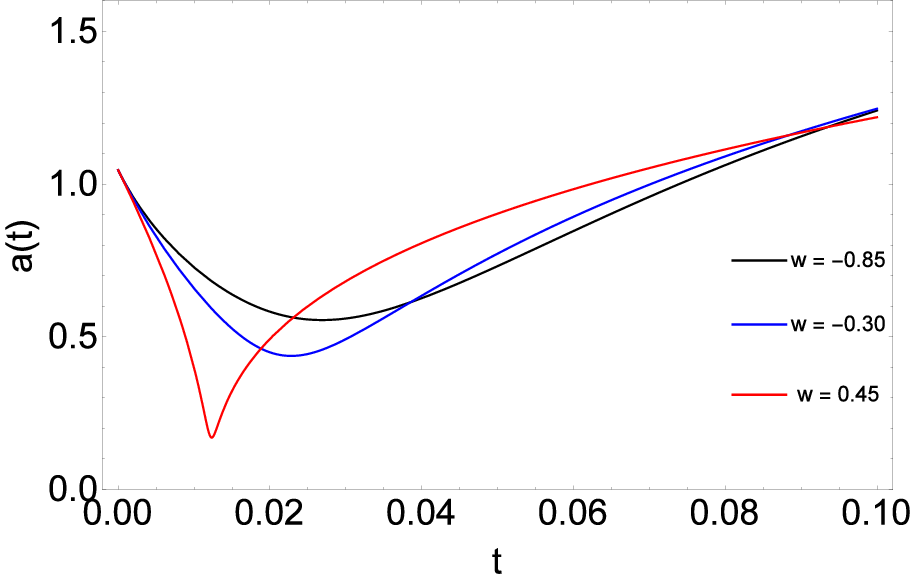
In the right panel of Fig. 2, we present the behavior of the scale factor for different values of the EoS parameter in the presence of non-commutative effects. It is seen that the EoS parameter controls the time interval at which the bounce occurs (hereafter we call it ) or more precisely the softness of the bounce66 6 The time interval for a soft bounce is much larger than a fast bounce.. As the EoS parameter changes its sign from negative to positive values, decreases leading to a fast bounce. Furthermore, the more negative the value of EoS parameter the less the minimum value for the scale factor at the bounce. It is worth mentioning that though the overall behavior of the curves in the right panel of Fig. 2 is similar (all the curves exhibit a bouncing scenario), the collapse dynamics and the location of horizons varies in response to the change in EoS and BD coupling parameters. Let us first deal with the collapse velocity. In the left and right panels of Fig. (3), we have plotted the collapse velocity for several values of EoS and BD coupling parameters. We see that, as the EoS increases from negative to positive values (fixing the parameter, see the upper panel), the collapse stops and turns faster to the expansion, with the bounce time getting advanced. Conversely, as the BD coupling parameter increases (fixing the EoS, see the right panel), the contracting phase turns faster to expansion with the bouncing time getting retarded.
The lower panel of Fig. 3 shows how the dynamical evolution of the collapsing body experiences one more phase compared to the dust case. Let us be more precise. For , the collapse scenario begins with an accelerated contracting phase ( and in the time interval ) till the first inflection point is reached at which and the collapse velocity has gained its maximum value in negative direction. The collapse then proceeds with a decelerating contracting phase before the bounce occurs, i.e., and , where . Just after the bounce occurs, the collapse turns to an accelerating expanding phase for which and that happens in the time interval . Finally, the dynamical evolution of the object ends through a decelerating expanding phase where and and .


III.2 Dynamics of the apparent horizon
In order to study the evolution of the apparent horizon, we begin by re-writing the spacetime metric (1) into the double null form as
| (30) |
with the null one-forms defined as
| (31) |
and we have transformed the spatial sector of the metric (1) from Cartesian coordinates to spherical coordinates with the area radius . The null vector fields dual to the null one-forms can be obtained easily as
| (32) |
The condition for radial null geodesics obeying equation implies the existence of two kinds of future pointing radial null geodesics, which correspond to and . The expansion factors along these geodesics are given by
| (33) |
The spacetime is said to be trapped, un-trapped or marginally trapped if, respectively [80]
| (34) |
where the equality characterizes the outermost boundary of the trapped region, the apparent horizon. Therefore, a shell labeled by the comoving radial coordinate will get trapped if , or equivalently
| (35) |
The left panel in Fig. 4 shows the behavior of the physical areal radius, , of the apparent horizon for the case of dust fluid. It is seen that when the effects of non-commutativity are present (full curve), the radius of the apparent horizon increases for a while and diverges just before the bounce where a contracting phase governs the scenario. It then decreases in the expanding phase to a minimum and monotonically increases at late times. From the above equation we can extract that, depending on the behavior of the collapse velocity, the horizons could either form or are avoided. This depends on how the initial radius of the collapsing object, i.e., , is chosen:
- •
Having taken the boundary of the collapsing cloud in such a way that , then Eq. (35) implies that once the absolute value of collapse speed and the scale factor reach the values (see also point A in the right panel of Fig. 4), the horizon equation is satisfied just once and a dynamical horizon would form to meet the boundary in the contracting phase. This means that the uttermost boundary of the trapped region will intersect the boundary of the collapsing cloud, i.e., .
- •
For or correspondingly when the absolute value of collapse speed and the scale factor reach the values (point B), two horizons could form; the first one in the collapsing phase and the second one in the expanding phase.
- •
However, for , since the horizon equation is satisfied once, only one horizon could form in the contracting regime and the post-bounce regime is free of horizon formation.
- •
Finally, for , the horizon equation is fulfilled three times where the absolute value of collapse speed and the scale factor assume the values (point C). The first one appears in the contracting phase, the second one in the accelerated expanding regime and the third one forms in the decelerated expanding regime to cover the bounce. We then conclude that the boundary surface of the collapsing body can be taken sufficiently small so that equation (35) is never satisfied, i.e., no horizon would develop to meet the boundary as the speed of collapse is always bounded (see the full curve in the right panel of Fig. 4). As a result, the formation of the horizon can be prevented in the presence of non-commutative effects. However, for (see dashed curve in the left panel of Fig. 4), the radius of the dynamical horizon decreases monotonically and vanishes at a finite amount of time. Thus, there can not be found a minimum radius for the boundary of the collapsing volume (since the collapse velocity is unbounded; see the dashed curve in the right panel of Fig. 4) in order to avoid the horizon formation.


III.3 Horizon location for non-dust case
Let us now check the location of dynamical horizons for . The left panel in Fig. 5 shows that the apparent horizon decreases for a while till the first inflection point, at which the absolute value of speed of collapse reaches its maximum value, at the corresponding value of the scale factor, in the contracting regime, (see also point D in the right panel). It then increases and diverges to infinity at the bounce time. After the bounce, the apparent horizon decreases again to its local minimum value at the second inflection point where the absolute value of the speed of the collapse reaches its maximum (Point E) in the post bounce regime, i.e., . The boundedness of the speed of collapse signals the fact that, depending on the suitable choice of the boundary surface of the collapsing body, formation of dynamical horizons can be avoided. Therefore, in view of the Fig. 5, we may deduce the following considerations:
- •
If we take the boundary to be , then no horizon would form throughout the dynamical evolution of the object, while the equality leads to the formation of only one horizon in the contracting phase.
- •
If we take then, two dynamical horizons would appear once the absolute value of the speed of collapse get the value at the corresponding values for the scale factor; the first horizon forms in the accelerated contracting regime once the point is reached and the second one forms at , after the first inflection point, where the collapse undergoes a decelerated contracting regime.
- •
For the expanding regime is free of horizon formation, since for this choice of the boundary surface, the horizon equation is never satisfied in the expanding regime.
- •
Finally, for , say , three horizons may form; the first one in the decelerated contracting regime (once the curve in plane reaches the point ). The second one occurs in the inflationary expanding regime, once the speed of collapse and the scale factor reach the point and finally, the third one would form at , after the second inflection point, i.e., in the decelerating expanding regime.
However, when the non-commutative effects are absent, the horizon formation cannot be avoided as te speed of the collapse is unbounded and a dynamical horizon would always form to cover the resulted singularity (see the dashed curve).


III.4 Oscillatory bounce, special cases and complementary perspective
In Fig. 6, we have plotted the time behavior of the scale factor associated to dust cloud collapse for large values of the BD coupling parameter. We find that there is a critical value for the non-commutative parameter such that when , the scale factor reaches a minimum value and stays at this value till late times (family of black curves). However, when this parameter is less than , the collapse culminates in a singularity formation with quite different dynamics during its evolution (see the family of red and blue curves) in comparison to the case where (gray curve). Although different initial collapse settings imply different numerical values for (for instance, the initial conditions chosen for plotting Fig. 6 give ), it should be noted that the mentioned behavior is completely general and does not depend on the initial conditions at all.

Fig. 7 presents the time behavior of BD scalar field for both non-commutative and commutative settings for a dust cloud. While for the former the BD field increases monotonically, for the latter, it undergoes a sudden divergence at the singularity time.

Another class of solutions concerns the collapse of dust fluid for negative values of the BD coupling parameter. The left plot in Fig. 8 presents the behavior of scale factor for both non-commutative and commutative settings. As the full curve shows, the scale factor decreases for a while, reaching a time at which an oscillatory bounce begins. It then increases by keeping this oscillatory behavior at the later times. The dashed curve shows the singular behavior for a vanishing value of the non-commutative parameter. The right panel shows the behavior of the collapse velocity, where we see that it begins oscillating in the negative direction before the bounce, at which the speed of collapse vanishes and proceeds this oscillatory behavior around its vanishing value. The inset shows the late time behavior of the collapse velocity, where it is seen that at early stages of the collapse the frequency of oscillation of is high and then it decreases at late times. Furthermore, the envelope of the oscillatory phase shows a damping as the time advances, which corresponds to the case where the collapsing body settles at rest at late times. Such a behavior in the dynamics of the collapse is due to the highly non-linear characteristic of the non-commutative equations.
Finally, in Fig. 9, we have shown the time evolution of Hamiltonian constraint, where we see that this constraint is fulfilled with the accuracy of or less.


III.5 Exterior solution
The collapse setting studied so far deals with the interior of the collapsing cloud. In order to complete the model we need to match the interior spacetime to a suitable exterior one. Let us take as four dimensional spacetimes and as a timelike three dimensional hypersurface that divides spacetime into two regions (exterior) and (interior). The line element for the exterior spacetime is taken as that of generalized Vaidya metric [81] which in retarded (exploding) null coordinates is given by
| (36) |
where being the exterior metric function with and being the Vaidya radius and retarded null coordinate, respectively. We label the exterior coordinates as . The interior line element (1) in spherical coordinates reads
| (37) |
where we have labeled the interior coordinates as . The hypersurface with intrinsic coordinates results from the isometric gluing of two hypersurfaces and , which, respectively, bound the exterior and interior regions. Utilizing generalized Israel-Darmois junction conditions [82] we proceed to match the above line element to the exterior one through the boundary surface . The induced metrics on and will take the following form, respectively
| (38) |
and
| (39) |
The junction conditions for the first fundamental forms (induced metrics) give
| (40) |
where an overdot denotes . In order to calculate the extrinsic curvature tensors of and , we need to find the unit vector fields normal to these hypersurfaces. We then get
| (41) |
The extrinsic curvature tensors associated with are given by
| (42) |
where and are parametric relations for the hypersurfaces and and are the components of connections associated to interior and exterior line elements. The junction conditions in BD theory have the form [82]
| (43) | |||||
| (44) |
where the notation stands for the jump of given field across the hypersurface , labels the coordinate normal to this surface and is the energy-momentum tensor of matter fields (except the BD scalar field) on the shell located at where and are the surface density of mass-energy and surface pressure, respectively. The quantities and are traces of and , respectively. We also note that equation (43) can be rewritten in an equivalent form as
| (45) |
A straightforward but lengthy calculation leads to the following expressions for the components of extrinsic curvature tensors, as
| (46) | |||||
| (47) |
Next, we proceed to compute the components of equation (45). We then get
| (48) |
The first part leaves us with the following expression for surface density in terms of extrinsic curvature components, as
| (49) |
while for the second part we get
| (50) |
where only non-vanishing components of the extrinsic curvature tensors have been considered. These equations can also be re-written in the following form as
| (51) |
The jump for the normal derivative of the BD scalar field across is found as
| (52) | |||||
where use has been made of the contravariant components of the normal vector fields
| (53) |
Thus, from equation (44), the jump in the normal derivative of BD scalar field and its continuity across we obtain
| (54) |
Equations (40), (51) and (54) fully determine the dynamics of the boundary, the exterior metric function and BD scalar field in the exterior region, once we know the matter distribution on the boundary. Assuming the boundary surface is devoid of mass-energy density and pressure, i.e., and , we get and if . Therefore, the continuity of and components of extrinsic curvature across leaves us with following relations for exterior quantities, as
| (55) | |||||
| (56) |
where use has been made of relations given in (40). Taking derivatives of (55) and the first part of (40) we get
| (57) |
whence we have
| (58) |
Substituting for and from the above relations into (56) we finally get
| (59) |
which implies that . Solving equations (55) and the first part of (40) we obtain the four-velocity of the boundary as
| (60) |
where we have chosen the minus sign for as we deal with a collapse setting. The continuity of the BD scalar field implies that this field must be homogeneous in the exterior region, i.e., . Taking this into account together with the first part of equation (54) gives which implies the BD scalar field outside the collapsing cloud is constant. We therefore conclude that the exterior region is a static spacetime with dynamical boundary. The process of finding the exterior metric function on the boundary passes through utilizing the Hamiltonian constraint, the equation of motion of the scale factor (25), the junction condition for induced line elements (the second part of (40)) and the trajectory equation for the boundary. Such a procedure may not be a simple task. However, we may intuitively deduce that the effects of phase space deformation could appear in the exterior spacetime as we solve the radial component of the four-vector velocity to find . From the second part of (40) and radial component of the four-vector velocity we get . The location of horizon from the exterior view is given by the condition . Therefore, the horizon would interest the boundary surface if the collapse velocity satisfies
| (61) |
whereby it is seen that if the collapse velocity is bounded, the boundary of the collapsing cloud can be chosen so that the formation of horizon is avoided. Such a scenario could occur within the non-commutative setting we presented here, whereas for commutative case, the collapse velocity diverges and the horizon would always form to cover the resulted singularity.
IV concluding remarks
In this paper, we have investigated the collapse process of a homogeneous perfect fluid in the context of the BD theory in deformed phase space. Let us clarify (further to our comments in in section I) why we have investigated in this paper a collapse scenario in a BD noncommutative setting instead of a corresponding one in GR. On the one hand, a collapse scenario in noncommutative GR has already been discussed in previous publications [64]. On the other hand, from another complementary perspective, let us add the following. It is well known that scalar tensor theories such as the BD theory can agree with GR in the post-Newtonian limit [11]. However, it should be emphasized that in a strong field setting77 7 As two appropriate examples of such strong field settings, we can mention the generation of the gravitational waves and the formation of the black holes and singularities during gravitational collapse, see, e.g., [11] and references therein., those theories may yield very different predictions. That may mean a few experimental and observational features, but also important different structural implications of these theories. In particular, we can allude to the formation of a singularity and black hole during gravitational collapse. This has been specifically investigated in the herein work. Considerable differences and relevant features were extracted, demonstrating how a noncommutative BD setting is much different from the corresponding standard BD theory as well as GR. Intrinsic to such difference is the fact that a scalar tensor gravitation involves more degrees of freedom, therefore, it yields a larger number of solutions than GR [11]. Moreover, the employed noncommutative parameter in the BD theory also couples to variables which are absent in the GR, and therefore, the range of solutions and possible scenarios is much wider. It was this broad scope of possibilities we investigated herein, regarding a collapse scenario in a BD noncommutative setting.
Assuming the interior geometry of the collapsing cloud to be that of a spatially flat FLRW spacetime, we employed a particular type of non-commutativity between the phase space coordinates and examined its effects on the collapse dynamics. More precisely, we have introduced in (17) a modified Poisson algebra in the Hamiltonian formalism.
Our numerical analysis shows that there are two different type of solutions which depend effectively on the sign of the BD coupling parameter. In the case where the BD coupling parameter is negative, oscillatory behaviors appear. However, by assuming positive values for , when the constant non-commutative parameter is absent, the collapse scenario is terminated at a spacetime singularity, whilst, for small values of the non-commutative parameter, there is a nonzero minimum value for the scale factor where the collapse halts and then an expanding phase begins.
For small values of the non-commutative parameter,88 8 In order to study appropriately the behavior of the quantities involved within the collapse setting and have a correct comparison among them as well as with the standard commutative models, we have taken the non-commutative parameter to be the same for all numerical plots. However, it is important to note that, for the variety of values, which can be taken by , they have also been examined both for the general case (according to left panel of Fig. 2) and also for particular case (large values of the BD coupling parameter), as seen in Fig. 6. both the EoS and BD coupling parameters can effectively control the dynamics of the collapse setting (see Fig. 2 and Fig. 3). More precisely, for small values of , the softness of the bounce depends effectively on the values taken by , i.e., matter pressure, and . For a non-dust case, as the pressure of the fluid tends to positive values, the collapse dynamics is altered such that the location and the number of the dynamical horizons are changed. Such a situation similarly happens as the BD coupling parameter increases (for a fixed value of EoS parameter).
The strength of the scalar to tensor coupling to the matter is encoded in the BD coupling parameter so that the smaller the value of parameter, the larger the contribution of the scalar field to gravitational interaction. As we found in the herein model, the coupling of the scalar to tensor field to matter content could affect the softness of the bounce and the time interval during which the bounce occurs. In this manner we could say that the stronger the contribution of the BD scalar field to the gravitational interaction (i.e., the parameter decreases), the softer the bounce occurs.
The behavior of the apparent horizon curve for a dust collapse has been also analyzed according to Figs. 4 and 5. It is seen that the dynamics of the apparent horizon in the case in which non-commutative effects are present is quite different to the case where these effects are absent. More concretely, when the non-commutative parameter takes small values, the formation or otherwise of the dynamical horizons depend crucially on the behavior of the collapse velocity.
Recent observations of radiation damping in mixed binary systems have put limitations on the BD coupling parameter as from the Cassini measurements [83]. In our scenario, we have shown that when takes very large values99 9 When goes to infinity, the BD theory may reduce to the GR [84]., we can find a critical value for the non-commutative parameter, i.e., , which completely disassociates two different dynamical behaviors for the collapsing object, see Fig. 6. More precisely, for , the scale factor decreases till reaching a minimum value and stays at this value as the time evolves. Whilst, for , the collapse culminates in a spacetime singularity with completely different dynamics compared to the case where the non-commutative effects are absent. It should be noted that the value of depends on the initial values which are taken by the present parameters of the model.
We have also studied the collapse associated to a pressureless fluid for negative values of the BD coupling parameter. As the left panel in Fig. 8 indicates, the scale factor starts its decreasing behavior till reaching the bounce, beyond which an increasing oscillatory behavior commences. The collapse velocity experiences an oscillatory phase such that at the earlier times, it oscillates toward its first vanishing point at the time (see the right panel of Fig. 8). Note that the speed of collapse remains negative for . It is therefore the acceleration of the collapse that changes its sign rapidly, signaling that the collapsing object experiences a series of decelerating (see the red arrow heading upward from points A to B) and accelerating (see the blue arrow heading downward from the points B to C) contracting regimes with a soft jump from the former to the latter (at point B) but a quick jump from the latter to the former (at point A or C). For the scenario enters an accelerated expanding phase for the first time (at ) and remains in this regime in the time interval . It then goes again under a decelerated expanding phase between till it enters an accelerated contracting phase which occurs for . This oscillatory behavior continues around the zero point velocity. We should note that the frequency of the oscillation of collapse velocity decreases with time.
Moreover, the corresponding envelop of the oscillatory phase is also damping with time. It is also worth mentioning that there exists a difference between the behavior of collapse velocity for this case and the case where . In the former, though the scale factor vanishes at a finite amount of time (singular behavior), the speed of collapse is limited (see the dashed curve in the right panel of Fig. 8) so that by a suitable choice of the boundary of the collapsing body, the formation of the apparent horizon can be avoided. Thus, the collapse may culminate in a naked singularity. For the latter, the collapse velocity diverges in the limit of approach to the singularity and the apparent horizon would always form to cover the resulting singularity. The lower panel in Fig. (8) shows the collapse velocity for different values of BD coupling parameter. It is seen that the larger the negative value of parameter, the smaller the frequency of oscillation.
To complete the collapse model, we performed matching the interior spacetime with that of generalized Vaydia spacetime using the generalized Israel-Darmois junction conditions. We observed that as long as there is no surface stress energy on the boundary of the collapsing cloud, the extrinsic curvature tensor is continuous across the boundary. This makes the exterior spacetime to be static with a dynamical boundary so that the horizon could intersect the boundary depending on the initial size of the collapsing body. Thus, if the initial size of the collapsing object is taken as small as enough, horizon formation could be avoided. We then conclude that the process of gravitational collapse in the presence of non-commutativity would lead to a non-singular bounce, that is uncovered by the horizon and so it can be causally connected to an external observer.
We would like to compare our results to other collapse scenarios as reported in the literature. Work along this line has been done within the gravity models which correspond to the BD theory with a vanishing coupling parameter, using the metric formalism. In this context, it has been shown that the collapse process of a perfect fluid leads to a spacetime singularity which can be either hidden behind a horizon or visible to external observers [67]. Besides the model presented here, non-singular bouncing scenarios have also been reported in the literature such as theories in Palatini formalism [85], generalized teleparallel gravity theories [86], bouncing models in the presence of interacting spinning particles in the framework of Einstein-Cartan theory in both cosmological [87] and astrophysical scenarios [88]. Non-singular bouncing scenarios have also been reported in loop quantum cosmology for a massless scalar field [89] and in the presence of anisotropy [90] (see also [91] and references therein).
Finally, we should be aware of the following notes about the herein model: (i) All the results of this paper have been obtained for a simple case in which we have introduced a constant non-commutative parameter within the standard BD theory, a homogeneous matter distribution and a spatially flat FLRW line-element for the interior region suitably matched to a generized Vaidya spacetime as the exterior solution. It would be interesting to extend the herein model by introducing other Poisson brackets instead of (17), other kinds of matter or geometry and/or other extended scalar-tensor theories. (ii) As it has been shown in section (II), the new quantities and have been redefined such that we obtained dimensionless quantities. In this rescaled setting, it is important to note that, in order to get an appropriate noncommutative scenario, we should not think that must take very small values (of orders the Planck length), but instead, it is enough to consider such that it is restricted to the interval . (iii) As the field equations in the Einstein representation do not contain second derivatives of , thus, this representation can be appropriate to extend predictions from GR to BD theory, especially in the vacuum case [11]. However, deriving the equations associated to the Einstein frame for our model (the same as obtaining the perturbed equations) is not easy to perform and we have not investigated them.
V ACKNOWLEDGMENTS
S. M. M. Rasouli is grateful for the support of grant SFRH/BPD/82479/2011 from the Portuguese Agency Fundação para a Ciência e Tecnologia. This research work was supported by the grant PEst-OE/MAT/UI0212/2014.
Appendix A On the Field equations in Non-Commutative Brans-Dicke Theory
For stiff fluid , equation (27) leaves us with a constant of motion as . Multiplying equation (26) by and equation (28) by , after adding up the results, we get
| (62) |
The right hand side of the above equation can be expanded near the bounce, where and . We then get, up to the first order
| (63) |
whence integration in the neighborhood of the bounce point gives
| (64) |
where is an integration constant. Substituting the above approximation into equation (26) and after a few algebra we find near the bounce
| (65) |
It is seen that the BD scalar field has a parabolic behavior near the bounce point. This behavior has been sketched in Fig. 10 where we see that the scalar field behaves parabolically near the bounce time .

Next, we can evaluate equation (25) at the bounce point which yields
| (66) |
Now, with the help of equations (64) and (65), we arrive at the following cubic equation for the bounce time as
| (67) |
where
| (68) |
Setting and taking the terms in (67) up to , we get the solution for the bounce time as (we assume )
| (69) |
The first solution is not acceptable as for a physically reasonable collapse setting we require that . We therefore take the second one as the bounce time. Furthermore, the case of vanishing does not display a bouncing scenario.
For a dust fluid, Eq. (27) can be immediately integrated to give
| (70) |
Multiplying equation (26) by and equation (28) by and after adding up the results we have
| (71) |
By differentiating equation (26) together with employing Eqs. (70) and (71), after a straightforward but lengthy calculation we arrive at the evolution equation for BD scalar field as
| (72) |
Similarly, we have found the acceleration equation for the collapse scenario as
| (73) | |||||
where we have neglected the terms containing . In order to complete the above set of equations, we need to substitute for and its derivative from equation (28). However, such a complicated process can not be done analytically and needs numerical considerations.
References
- [1] V. Faraoni, Cosmology in Scalar Tensor Gravity, KLUWER ACADEMIC PUBLISHERS (2004).
- [2] C. Brans and R. H. Dicke, Phys. Rev. 124, 925 (1961).
- [3] K. Gdel, Rev. Mod. Phys. 21 447 (1949).
- [4] I. Ozvath, E. Schcking, in Recent Developments in General Relativity, (Pergamon, New York, 1962).
- [5]
P. Jordan, Projective Relativity (Friedrich Vieweg und Sohn, Braunschweig, 1955).
P. Jordan, Z. Phys. 157 112 (1959);
D. R. Brill, Evidence for Gravitational Theories, Enrico Fermi Course XX, Ed. C. Moiler (Academic Press, New York 1962) p. 50-68;
Y. Fujii and K.-Ichi Maeda, The Scalar-Tensor Theory of Gravitation, Cambridge University Press 2003;
S. Capozziello and V. Faraoni, Beyond Einstein Gravity, A Survey of Gravitational Theories for Cosmology and Astrophysics, Springer Science + Business Media 2011;
V. Faraoni, E. Gunzig and P. Nardone, Fundam. Cosmic Phys. 20, 121 (1999). - [6]
C. M. Will, Theory and Experiment in Gravitational Physics (Cambridge University Press, Cambridge, England, 1993);
Living Rev. Relativity 9 3 (2006). - [7] T. Matsuda and H. Nariai, Prog. Theor. Phys. 49 1195 (1973).
- [8] M. Shibata, K. Nakao and T. Nakamura, Phys. Rev. D 50 7304 (1994).
- [9] S. W. Hawking, Commun. Math. Phys. 25, 167 (1972).
- [10] T. P. Sotiriou and V. Faraoni, Phys. Rev. Lett. 108 081103 (2012).
- [11] M. A. Scheel, S. L. Shapiro and S. A. Teukolsky, Phys. Rev. D, 51 4208 (1995); Phys. Rev. D 51, 4236 (1995).
- [12] G. Kang, Phys. Rev. D 54, 7483 (1996).
- [13] K. S. Thorne and J. J. Dykla, Astrophys. J. 166 L35 (1971).
- [14] T. Jacobson, Phys. Rev. Lett. 83, 2699 (1999).
- [15] O. J. Kwon, Y. D. Kim, Y. S. Myung, B. H. Cho and Y. J. Park, Phys. Rev. D 34, 333 (1986).
- [16] M. Campanelli and C. O. Lousto, Int. J. Mod. Phys. D 2, 451 (1993).
- [17] A. G. Agnese and M. La Camera, Phys. Rev. D 51, 2011 (1994).
- [18] T. Chiba and J. Soda, Prog. Theor. Phys. 96 567 (1996).
- [19] T. Harada, T. Chiba, K.-I. Nakao and T. Nakamura, Phys. Rev. D 55 2024 (1997).
- [20] K. K. Nandi, Bhattacharjee, S. M. K. Alam and J. Evans, Phys. Rev. D 57, 823 (1998).
- [21] H. Kim, Phys. Rev. D, 60 024001 (1999).
- [22] H. Saida and J. Soda, Class. Quant. Grav. 17 4967 (2000).
- [23] N. Sakai and J. D. Barrow, Classical Quantum Gravity 18, 4717 (2001).
- [24] T. Harada, C. Goymer and B. J. Carr, Phys. Rev. D 66, 104023 (2002).
- [25] A. Bhadra, K. Sarkar, Gen. Rel. Grav. 37 2189 (2005).
- [26] Y. Gong and A. Wang, Phys. Rev. Lett. 99, 211301 (2007).
- [27] B. Nayak and L. P. Singh, Phys. Rev. D 80 023529 (2009).
- [28] D. Hwang and D. Yeom, Classical Quantum Gravity 27, 205002 (2010).
- [29] V. Faraoni, Entropy 2010 12, 1246 (2010).
- [30] N. Bedjaoui, P. G. LeFloch, J. M. Martin-Garcia and J. Novak, Class. Quant. Grav. 27 245010 (2010).
- [31] J. R. Morris, Gen. Relativ. Grav. 44 437 (2011)
- [32] P. Rudra, R. Biswas and U. Debnath, Astrophys. and Space Sci., 354 2101 (2014); arXiv:1307.6603 [physics.gen-ph]. Astrophys. and Space Sci., 339 135 (2012); arXiv:1203.1454 [gr-qc].
- [33] Y. S. Myung and T. Moon, Phys. Rev. D 89 104009 (2014).
- [34] M. Sharif and R. Manzoor, Mod. Phys. Lett. A 29 1450192 (2014).
- [35] J. Novak, Phys. Rev. D 57 4789 (1998).
- [36] H. S. Snyder, Phys. Rev 71 38 (1947); Phys. Rev 72 68 (1947).
- [37]
R. Banerjee, B. Chakraborty, S. Ghosh, P. Mukherjee and S. Samanta, Found. Phys. 39 1297 (2009);
I. Hinchliffe, N. Kersting and Y. L. Ma, Int. J. Mod. Phys. A 19 179 (2004). - [38]
M. R. Douglas and N. A. Nekrasov, Rev. Mod. Phys. 73 977 (2001);
R. J. Szabo, Phys. Rep. 378, 207 (2003). - [39] J. Polchinski, String Theory, (Cambridge University Press, Cambridge, 1998).
- [40] M. Heller, W. Sasin, arXiv:gr-qc/9906072; M. Patel, arXiv:math/0008023 [math.GM]; J. W. Moffat, Phys. Lett. B 493 142 (2000); C.-S. Chu, K. Furuta and T. Inami, Int. J. Mod. Phys. A 21 67 (2006); I. Bars, hep-th/0109132.
- [41]
S. M. Carroll, J. A. Harvey, V. A. Kostelecky, C. D. Lane,
and T. Okamoto, Phys. Rev. Lett. 87, 141601 (2001);
C. E. Carlson, C. D. Carone, and R. F. Lebed, Phys. Lett. B518, 201 (2001); 549, 337 (2002). - [42] J. M. Romero and J. D. Vergara, Mod. Phys. Lett. A 18, 1673 (2003).
- [43] V. P. Nair and A. P. Polychronakos, Phys. Lett. B 505 267 (2001), arXiv:hep-th/0011172; J. Gamboa, M. Loewe and J. C. Rojas, Phys. Rev. D 64 067901 (2001), arXiv:hep-th/0010220; S. Bellucci, A. Nersessian and C. Sochichiu, Phys. Lett. B 522 345 (2001), arXiv:hep-th/0106138; R. Banerjee, Mod. Phys. Lett A 17 631 (2002), arXiv:hep-th/0106280; B. Muthukumar and P. Mitra, Phys. Rev. D 66 027701 (2002), arXiv:hep-th/0204149 ; S. Samanta, Mod. Phys. Lett. A 21 675 (2006), arXiv:hep-th/0510138; S. Gangopadhyay and F. G. Scholtz, arXiv:0812.3474 [math-ph].
- [44] M. Chaichian and M. M. Sheikh-Jabbari, Phys. Rev. Lett 86 2716 (2001), arXiv:hep-th/0010175; X. Calmet, Eur. Phys. J. C 41 269 (2005), arXiv:hep-th/0401097; Z. Gur-alnik R. Jackiw, Pi, S.-Y. and A. P. Polychronakos, Phys. Lett. B 517 450 (2001), arXiv:hep-th/0106044.
- [45] J . Belissard, Lect. Notes in Physics 257 99 (1986); J. Belissard, A. Van Elst and H. SchulzBaldes, cond-mat/9301005.
- [46]
J. Gamboa, M. Loewe, F. Mendez and J. C. Rojas, Mod. Phys. Lett. A 16 2075 (2001);
J. Gamboa, M. Loewe, J. C. Rojas, Phys. Rev. D 64 067901 (2001). - [47]
N. Seiberg and E. Witten, JHEP 9909 032 (1999);
A. Connes, M. R. Douglas and A. Schwarz, JHEP 9802 003 (1998). - [48] H. Garcia-Compean, O. Obregon, C. Ramirez and M. Sabido, Phys. Rev. D 68 044015 (2003); Phys. Rev. D 68 045010 (2003); A. H. Chamseddine, J. Math. Phys. 44 2534 (2003); V. O. Rivelles, Phys. Lett. B 558 191 (2003); M. Maceda, J. Madore, P. Manousselis, and G. Zoupanos, Eur. Phys. J. C 36 529 (2004); P. Aschieri, M. Dimitrijevic, F. Meyer and J. Wess, Class. Quant. Grav. 23 1883 (2006); X. Calmet and A. Kobakhidze, Phys. Rev. D 72 045010 (2005); L. Alvarez-Gaume, F. Meyer and M. A. Vazquez- Mozo, Nucl. Phys. B 753 92 (2006); S. Estrada-Jimenez, H. Garcia-Compean, O. Obregon and C. Ramirez, Phys. Rev. D 78 124008 (2008); P. Aschieri and L. Castellani, J. Geom. Phys. 60 375 (2010).
- [49] J. M. Romero and J. A. Santiago, Mod. Phys. Lett. A 20 781 (2005), arXiv:hep-th/0310266.
- [50] R. Brandenberger and P.-M. Ho, Phys. Rev. D 66 023517 (2002), arXiv:hep-th/0203119; Q.-G. Huang and M. Li, J. Cosmol. Astropart. Phys. 11 001 (2003), arXiv:0308458 [astro-ph]; JHEP 06 014 (2003), arXiv:hep-th/0304203; H. Kim, G. S. Lee, and Y. S. Myung, Mod. Phys. Lett. A 20 271 (2005), arXiv:hep-th/0402018; H. Kim, G. S. Lee, H. W. Lee, and Y. S. Myung, Phys. Rev. D 70 043521 (2004), arXiv:hep-th/0402198; A. Kempf and L. Lorenz, Phys. Rev. D 74 103517 (2006); A. Ashoorioon, A. Kempf, and R. B. Mann, Phys. Rev. D 71 023503 (2005); Y. S. Myung, Phys. Lett. B 601 1 (2004), arXiv:hep-th/0407066; Dao-jun Liu and Xin-zhou Li, Phys. Rev. D 70 123504 (2004), arXiv:0402063 [astro-ph]; G. Calcagni, Phys. Rev. D 70 103525 (2004), arXiv:hep-th/0406006; Phys. Lett. B 606 177 (2005), arXiv:hep-th/0406057; Rong-Gen Cai, Phys. Lett. B 593 1 (2004), arXiv:hep-th/0403134; C.-S. Chu, B. R. Greene, and G. Shiu, Mod. Phys. Lett. A 16 2231 (2001), arXiv:hep-th/0010207; S. Tsujikawa, R. Maartens, and R. Brandenberger, Phys. Lett. B 574 141 (2003), arXiv:0308169 [astro-ph]; G. Calcagni and S. Tsujikawa, Phys. Rev. D 70 103514 (2004), arXiv:0407543 [astro-ph]; S. M. M. Rasouli and P. V. Moniz, Phys. Rev. D 90, 083533 (2014); S. M. M. Rasouli, M. Farhoudi and N. Khosravi, Gen. Rel. Grav. 43, 2895 (2011).
- [51] H. Garcia-Compean, O. Obregon, and C. Ramirez, Phys. Rev. Lett. 88, 161301 (2002), arXiv:hep-th/0107250.
- [52] G. D. Barbosa and N. Pinto–Neto, Phys. Rev. D 70; N. Khosravi, S. Jalalzadeh, H. R. Sepangi, Gen. Rel. Grav. 39 899 (2007).
- [53] A. Bina, S. Jalalzadeh, A. Moslehi, Phys. Rev. D 81 023528 (2010), arXiv:1001.0861 [gr-qc]; A. Bina, K. Atazadeh, S. Jalalzadeh, Int. J. Theor. Phys. 47 1354 (2008), arXiv:0709.3623 [gr-qc]; S. Pramanik, S. Ghosh, arXiv:1301.4042 [hep-th].
- [54] W. Kim and E. J. Son, Phys. Rev. D 75 024025 (2007); L. N. Chang, D. Minic, N. Okamura, and T. Takeuchi, Phys. Rev. D 65 125028 (2002).
- [55] N. Khosravi, S. Jalalzadeh and H. R. Sepangi, JHEP 01 134 (2006).
- [56] M. Maceda, J. Madore, P. Manousselis, G. Zoupanos, Eur. Phys. J. C 36 529 (2004); F. Finelli, JCAP 0310 (2003) 011; A. Chaney, L. Lu and A. Stern, Phys. Rev. D 92 064021 (2015).
- [57] G. D. Barbosa and N. Pinto–Neto, Phys. Rev. D 70 103512 (2004).
- [58] L. O. Pimentel and C. Mora, Gen. Rel. Grav., 37 817 (2005).
- [59] W. Guzman, M. Sabido, J. Socorro, Phys. Rev. D, 76 (2007), 087302; S. M. M. Rasouli, N. Saba, M. Farhoudi, J. Marto and P. V. Moniz, “In ationary Universe in a Deformed Phase Space Setting”, in progress.
- [60] N. Khosravi, S. Jalalzadeh and H.R. Sepangi, Int. J. Mod. Phys. D, 16 1187 (2007); JHEP, 0601 134 (2006).
- [61] T. Matsufuji and S. Naka, Progress of Theoretical Physics, 98, 3 (1997).
- [62] S. Kobayashi, Int. J. Mod. Phys. A, 31, 1650080 (2016).
- [63] C. Bastos, O. Bertolami, N.C. Dias and J.N. Prata, Phys. Rev. D 80 (2009) 124038.
- [64] P. Nicolini, arXiv:hep-th/0510203; P. Nicolini, A. Smailagic, and E. Spallucci, Phys. Lett. B 632 547 (2006); T. G. Rizzo, JHEP 09 (2006) 021; S. Ansoldi, P. Nicolini, A. Smailagic and E. Spallucci, Phys. Lett. B 645 261 (2007); P. Mukherjee and A. Saha, Phys. Rev. D 77 064014 (2008); R. Casadio and P. Nicolini, JHEP 11 (2008) 072; E. Spallucci, A. Smailagic and P. Nicolini, Phys. Lett. B 670 449 (2009); S. Ansoldi, Spherical black holes with regular center: a review of existing models including a recent realization with Gaussian sources, arXiv:0802.0330 [gr-qc]; P. Nicolini, Int. J. Mod. Phys. A 24 1229 (2009); I. A. Guerrero, D. Batic and M. Nowakowski, Class. Quant. Grav. 26 245006 (2009); A. Smailagic and E. Spallucci, Phys. Lett. B 688 82 (2010); C. Bastos, O. Bertolami, N. C. Dias and J. N. Prata, J. Phys. Conf. Ser. 314 012042 (2011); J. R. Mureika and P. Nicolini, Phys. Rev. D 84 044020 (2011); R. Garattini and B. Majumder, Nucl. Phys. B 884 125 (2014).
- [65] S. M. M. Rasouli, A. H. Ziaie, J. Marto, and P. V. Moniz, Phys. Rev. D 89, 044028 (2014).
- [66] L. E. Gurevich, A. M. Finkelstein and V. A. Ruban, Astrophys. Space Sci. 22 231 (1973); O. Hrycyna and M. Szydlowski, JCAP 12 016 (2013).
- [67] A. H. Ziaie, K. Atazadeh and Y. Tavakoli, Class. Quant. Grav. 27 075016 (2010); A. H. Ziaie, K. Atazadeh and S. M. M. Rasouli, Gen. Relativ. Gravit 43 2943 (2011); A. H. Ziaie, A. Ranjbar and H. R. Sepangi, Class. Quantum Grav. 32 025010 (2015).
- [68] C. W. Misner, K. S. Thorne and J. A. Wheeler, Gravitation, Freeman (1973); G. C. McVittie, Astrophys. J. 140 401 (1964).
- [69] S. Sen and A. A. Sen, Phys. Rev. D 63 124006 (2001).
- [70] S. M. M. Rasouli, M. Farhoudi and H. R. Sepangi, Classical Quantum Gravity 28, 155004 (2011); S.M. M. Rasouli, M. Farhoudi and P. V. Moniz, Classical Quantum Gravity 31, 115002 (2014). S. M. M. Rasouli, Prog. Math. Rel., Gravit. Cosmol. 60, 371 (2014).
- [71] P. S. Wesson, Space–Time–Matter: Modern Kaluza–Klein Theory (World Scientific, Singapore, 1999); N. doroud, S. M. M. Rasouli and S. Jalalzadeh, Gen. Rel. Grav. 41, 2637 (2009); S. M. M. Rasouli and S. Jalalzadeh, Ann. Phys. (Berlin) 19, 276 (2010).
- [72]
J. D. Brown, Classical Quantum Gravity 10 1579 (1993);
O. Bertolami, F. S. N. Lobo, J. Paramos, Phys. Rev. D 78 064036 (2008). - [73] M. R. Setare, Phys. Rev. D 70 087501 (2004); M. R. Setare, Int. J. Mod. Phys. A 21 1325 (2006); M. V. Battisti and G. Montani, Phys. Lett. B 656 96 (2007); M. V. Battisti and G. Montani Phys. Rev. D 77 023518 (2008).
- [74] A. E. F. Djemaï, H. Smail, Commun. Theor. Phys. 41 (2004) 837; A. E. F. Djemaï, Int. J. Theor. Phys. 35 (1996) 519.
- [75]
G. Esposito and C. Stornaiolo, Int. J. Geom. Meth. Mod. Phys. 4 (2007)
349 (arXiv: hep-th/0607114)
J. M. Gracia-Bondia, F. Lizzi, G. Marmo and P. Vitale, J. High Energy Phys. 0204 (2002) 026 (arXiv: hep-th/0112092). - [76] S. Minwalla, M. Van Raamsdonk, and N. Seiberg, JHEP 02 (2000) 020; M. Van Raamsdonk and Seiberg N., JHEP, 03 035 (2000); S. Minwalla, M. Van Raamsdonk and N. Seiberg, JHEP 0002: 020 (2000); A. Micu and M. M. Sheikh-Jabbari, JHEP 0101 025 (2001).
- [77] G. Amelino-Camelia, G. Gubitosi and F. Mercati, Phys. Lett. B 676 (2009) 180.
- [78] A. Eftekharzadeh and B. L. Hu, Braz. J. Phys. 35 (2005) 333.
- [79] W. Guzmán, M. Sabido and J. Socorro, Phys. Lett. B 697, 271 (2011).
- [80] S. Hayward, Phys. Rev. D 49 6467 (1994), arXiv:9303006[gr-qc]; ibid, Phys. Rev. D 53 1938 (1996), arXiv:9408002 [gr-qc]; C. W. Misner and D. H. Sharp, Phys. Rev. 136 B571 (1964); S. A. Hayward, Phys. Rev. D 49 831 (1994), arXiv:9303030 [gr-qc]. O. Bertolami and P. J. Martins, Phys. Rev. D 61 064007 (2000).
- [81] N. O. Santos, Mon. Not. Roy. Astron. Soc. 216 403 (1985); A. Wang and Y. Wu, Gen. Rel. Grav., 31 (1999) 107; S. D. Maharaj, G. Govender and M. Govender, Gen. Relativ. Gravit. 44 (2012) 1089.
- [82] K. G. Suffern, J. Phys. A: Math. Gen. 15 (1982) 1599; C. Barrabes and G. F. Bressange, Class. Quantum Grav. 14 805 (1997); F. Dahia and C. Romero, Phys. Rev. D 60 104019 (1999). J. D. Barrow and P. Parsons, Phys. Rev. D 55 (1997) 1906.
- [83] J. Alsing, E. Berti, C. M. Will and H. Zaglauer, Phys. Rev. D 85 (2012) 064041.
- [84] A. Barros and C. Romero, Phys. Lett. A 173, 243 (1993); N. Banerjee and S. Sen, Phys. Rev. D 56, 1334 (1997); V. Faraoni, Phys. Lett. A 245, 26 (1998); V. Faraoni, Phys. Rev. D 59, 084021 (1999). Supplement Series 53 (1983) 93; K. D. Kokkotas and J. Ruoff, Astron. Astrophys. 366 565 (2001).
- [85] C. Barragan, G. J. Olmo and H. Sanchis-Alepuz, Phys. Rev. D 80 (2009) 024016.
- [86] Yi-Fu Cai, Shih-Hung Chen, J. B. Dent, S. Dutta and E. N. Saridakis, Class. Quantum Grav. 28 (2011) 215011.
- [87] S. D. Brechet, M. P. Hobson, A. N. Lasenby, Class. Quantum Grav. 25 (2008) 245016.
- [88] A. H. Ziaie, P. V. Moniz, A. Ranjbar, H. R. Sepangi, arXiv:1305.3085 [gr-qc].
- [89] A. Ashtekar, T. Pawlowski and P. Singh, Phys. Rev. Lett. 96 (2006) 141301; ibid, Phys. Rev. D 73 (2006) 124038; ibid , Phys. Rev. D 74 (2006) 084003.
- [90] A. Ashtekar and E. Wilson-Ewing, Phys. Rev. D 79 (2009) 083535; ibid Phys. Rev. D 80 (2009) 123532; E. Wilson-Ewing, Phys. Rev. D 82 (2010) 043508; M. Martin-Benito, G. A. Mena Marugan and T. Pawlowski, Phys. Rev. D 78 (2008) 064008; ibid Phys. Rev. D 80 (2009) 084038.
- [91] A. Ashtekar and P. Singh, Class. Quantum. Grav. 28 (2011) 213001. 366 (2001) 565;V. K. Gupta, V. Tuli and A. Goyal, Astrophys. J. 579 (2002) 374; A. Brillante and I. N. Mishustin, EPL 105 (2014) 39001.